Abstract

Transitions from classical to quantum behaviour in a spin system with two degenerate ground states separated by twin energy barriers which are asymmetric due to an applied magnetic field are investigated. It is shown that these transitions can be interpreted as first– or second–order phase transitions depending on the anisotropy and magnetic parameters defining the system in an effective Lagrangian description.

1 Introduction

Barrier penetration by tunneling processes is a purely quantum phenomenon which does not arise in classical physics where only processes leading over the barrier, e.g. thermal activity according to a classical Boltzmann distribution, yield a nonzero barrier transition rate. At finite temperature, either tunneling from thermally excited states (“temperature assisted tunneling”) or thermal fluctuations over the barrier (“thermal activity”) dominate the transition rate, and the crossover from temperature assisted tunneling to thermal activity can be understood as a phase transition from the quantum phase to the classical phase of a physical system which is of either first or second order.

Whereas the general theory of these phase transitions in an abstract potential barrier setting is well known and clearly understood [1] (there is a remarkable similarity to the Maxwell theory of phase transitions in the Van der Waals gas), only very few models are known which allow an explicit and analytic investigation of the phase transitions in decay and transition rates which may even be accessible to experimental verification. Hence the recent discovery that spin systems provide examples which exhibit first– and second–order phase transitions [2] aroused interest in the investigation of such systems. In particular, a large spin in an $X0Y$ easy plane anisotropy with easy $y$–axis can be shown to exhibit both first– and second–order phase transitions depending on the value of the anisotropy parameter.

In the following, we consider this spin system with an additional applied magnetic field and investigate its influence on the dominant transition process. We begin with the presentation of the model and its effective semiclassical Lagrangian in Section 2, and then review the theory of temperature assisted quantum tunneling and thermal activity in Section 3. Section 4 contains some analytical results which guided the numerical calculations presented in Section 4 and discussed in the concluding Section 5.

2 The model and its semiclassical approximation

We consider a giant spin in an $X0Y$ easy plane anisotropy with easy axis along the $x$–direction and external magnetic field B in the $y$–direction, perpendicular to the easy direction. The corresponding Hamiltonian $\hat{H}$ involves the spin operator $\hat{\vec{S}}$ and is given by [3, 4]

$$\hat{H}=K(\hat{S}_{z}^{2}+\lambda\hat{S}_{y}^{2})-2\mu_{B}{\cal B}\hat{S}_{y}$$ (1)

where the easy $xy$–plane demands $\lambda<1$.

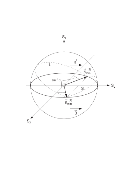
Figure 1: Classical visualization of the $X0Y$–easy plane $x$–easy axis spin system with applied magnetic field in the $y$–direction.

The physical situation described by this Hamiltonian is illustrated in Fig. 1 where the spin operator is represented as a classical spin vector $\hat{S}\in{\bf S}^{1}$. For zero magnetic field ${\cal B}=0$ the ground state is twofold degenerate, the classical spin vector pointing along the positive or negative $x$–direction, i.e. along the easy axis.

Under the influence of an applied magnetic field in the $y$–direction, there are still two degenerate spin ground state directions $\vec{S}^{(1)}_{min}$, $\vec{S}^{(2)}_{min}$ in the easy $xy$–plane moving towards the $y$–direction with increasing field ${\cal B}$.

To change the direction of the spin from one of these ground state directions to a neighbouring one, one has to avercome an energy barrier, moving the spin along either path $S$ or path $L$.

To study quantum tunneling and classical thermal effects of the discrete spin system described by $\hat{H}$, we convert the spin operators to a continuous potential problem. This can be achieved with the help of spin coherent state path integrals [5] or using the Villain transformation [6]. Both approaches yield a semiclassical description of the quantum system given by the effective Lagrangian

$${\cal L}(\phi,\dot{\phi})=\frac{1}{2}M(\phi)\dot{\phi}^{2}-V(\phi)$$ (2)

where

$$V(\phi)=K\lambda s^{2}(\sin^{2}\phi-\alpha)^{2}$$ (3)

and

$$M(\phi)=\frac{1}{2K(1-\lambda\sin^{2}\phi+\alpha\lambda\sin\phi)},\quad\alpha:=\frac{\mu_{B}\cal{B}}{K\lambda s}.$$ (4)

Here $\phi$ may be interpreted as a spherical parameter of the classical spin vector

$$\vec{s}=s(\sin\theta\cos\phi,\sin\theta\sin\phi,\cos\theta).$$ (5)

The semiclassical approximation is exact in the limit of large spin, $s\rightarrow\infty$, in the entire range of the anisotropy parameter $\lambda$, $0<\lambda<1$ [7].

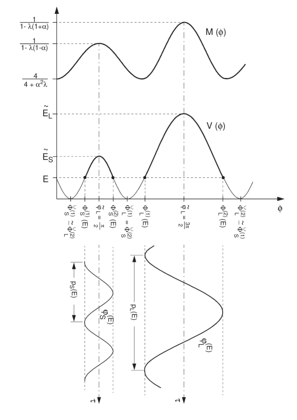
Figure 2: Asymmetric twin barrier potential $V(\phi)$, field dependent mass $M(\phi)$ and small and large barrier periodic instantons.

The shape of the potential $V(\phi)$ is shown in Fig. 2, together with the field–dependent mass $M(\phi)$ which is a special feature of this model. For small magnetic and anisotropy parameters, i.e. $\lambda\ll 1$, $\alpha\ll 1$, one can approximate the mass function by a constant value $M(\phi)\approx\frac{1}{2K}$ [4], but we are here particularly interested in the effect of nonconstant mass on quantum tunneling and thermal activity. Therefore we restrict the mass only to be positive which yields the condition $\lambda(1+\alpha)<1$ for the magnetic parameter $\alpha$, but keep the full $\phi$–dependence of $M(\phi)$.

The degenerate spin ground states are given by the two different types of minima of $V(\phi)$ at $2l\pi+\arcsin\alpha$ and $(2l+1)\pi-\arcsin\alpha$. These minima are separated by a small barrier $S$ with height

$$V\left(\frac{\pi}{2}\right)=K\lambda s^{2}(1-\alpha)^{2}=:\tilde{E}_{S}$$ (6)

and a large barrier $L$ with height

$$V\left(\frac{3\pi}{2}\right)=K\lambda s(1+\alpha)^{2}=:\tilde{E}_{L}$$ (7)

which correspond to the paths $S$ and $L$ shown in Fig. 1.

Since $\phi$ and $\phi+2\pi$ describe the same physical state, we restrict ourselves to the first twin barrier pair at $\tilde{\varphi}_{S}=\frac{\pi}{2}$ and $\tilde{\varphi}_{L}=\frac{3\pi}{2}$. The maximum positions $\tilde{\varphi}_{S}$ and $\tilde{\varphi}_{L}$ are called “sphalerons” in the usual field theoretical terminology. The vacua surrounding these barriers are denoted by

$$\breve{\Phi}^{(1)}_{S}=\arcsin\alpha\simeq\breve{\Phi}^{(2)}_{L}=2\pi+\arcsin\alpha$$ (8)

and

$$\breve{\Phi}^{(2)}_{S}=\pi-\arcsin\alpha=\breve{\Phi}^{(1)}_{L}.$$ (9)

We observe that barriers of different height only exist for $0<\alpha<1$. For vanishing magnetic field ($\alpha=0$), the two barriers are equally high [8], whereas in the limit $\alpha\rightarrow 1$, the magnetic field dominates the easy axis effect and there is only one ground state pointing along the $y$–direction.

3 The theory of quantum tunneling and thermal activity

We consider transitions between spin states built around the two degenerate vacua at finite temperature, i.e. we assume the quantum spin states to be populated according to a Boltzmann distribution.

The rate of thermal activity over the small or large barrier is to first order given by the Boltzmann factor,

$$\tilde{\Gamma}_{i}(T)\sim e^{\tilde{S}_{i}(T)},\qquad\tilde{S}_{i}(T):=\frac{\tilde{E}_{i}}{T}$$ (10)

with $i=S,L$ and $k_{B}=1$. $\tilde{S}_{S}(T)$ and $\tilde{S}_{L}(T)$ are called the thermodynamic actions of the small and the large barrier, respectively.

The temperature assisted tunneling rate can be estimated by a Boltzmann average over the tunneling probabilities from excited states with energy $E$. These tunneling probabilities can be approximated by the semiclassical WKB exponents, $P_{i}(E)=e^{-W_{i}(E)}$,

$$W_{i}(E)=2\sqrt{2}\int_{\Phi_{i}^{(1)}(E)}^{\Phi_{i}^{(2)}(E)}\sqrt{M(\phi)(V(\phi)-E)}d\phi,\qquad i=S,L$$ (11)

where $\Phi_{S}^{(1,2)}(E)$, $\Phi_{L}^{(1,2)}(E)$ are the turning points for the small ($S$) or large ($L$) barrier at energy $E$, i.e. the solutions of the equation $V(\phi)=E$. It is easy to see that

$$\Phi_{S}^{(1)}(E) = \arcsin\left(\alpha+\sqrt{\frac{E}{K\lambda s^{2}}}\right)$$

$$\Phi_{S}^{(2)}(E) = \pi-\arcsin\left(\alpha+\sqrt{\frac{E}{K\lambda s^{2}}}\right)$$

$$0\leq E\leq E_{S}$$ (12)

and $\displaystyle\Phi_{L}^{(1)}(E)$ $\displaystyle=$ $\displaystyle\pi-\arcsin\left(\alpha-\sqrt{\frac{E}{K\lambda s^{2}}}\right)$ $\displaystyle\Phi_{L}^{(2)}(E)$ $\displaystyle=$ $\displaystyle 2\pi+\arcsin\left(\alpha-\sqrt{\frac{E}{K\lambda s^{2}}}\right)$ $$0\leq E\leq E_{L}.$$ (13)

Taking the Boltzmann average over the tunneling probabilities from excited states $P_{i}(E)$ yields the temperature assisted tunneling rate,

$$\Gamma_{i}(T)=\int_{0}^{\infty}dEe^{-\frac{E}{T}}P_{i}(E)=\int_{0}^{\infty}dEe^{-\frac{E}{T}-W_{i}(E)}.$$ (14)

This integral can be estimated by the steepest descent method, using the concept of periodic instantons [1, 9]. These are classical solutions of the Euclidean Euler–Lagrange equations of the semiclassical Lagrangian (2), i.e.

$$M(\phi)\ddot{\phi}+\frac{1}{2}\frac{dM(\phi)}{d\phi}\dot{\phi}-\frac{dV(\phi)}{d\phi}=0$$ (15)

(dots now denote derivatives with respect to Euclidean time $\tau=it$) with finite energy $E$ as integration constant in the first integral,

$$\frac{1}{2}M(\phi)\dot{\phi}^{2}-V(\phi)=-E.$$ (16)

For $0<E<\tilde{E}_{S}$ or $0<E<\tilde{E}_{L}$ there are solutions $\varphi^{E}_{S}(\tau)$, $\varphi^{E}_{L}(\tau)$ oscillating around the small or large barrier with period $p_{S}(E)$, $p_{L}(E)$, respectively. These solutions can be derived by integrating eq. (16) which leads to elliptic integrals, but it is impossible to solve the resulting expressions for the explicit $\tau$–dependence of the solutions $\varphi^{E}_{S}$, $\varphi^{E}_{L}$ which are visualized in Fig. 2.

Nonetheless it is possible to compute the periods and the Euclidean actions of these periodic instantons from eq. (16) which yields

$$p_{i}=\sqrt{2}\int_{\Phi_{i}^{(1)}(E)}^{\Phi_{i}^{(2)}(E)}\sqrt{\frac{M(\phi)}{V(\phi)-E}}d\phi$$ (17)

and

$$S_{i}=2\sqrt{2}\int_{\Phi_{i}^{(1)}(E)}^{\Phi_{i}^{(2)}(E)}\sqrt{M(\phi)(V(\phi)-E)}d\phi+p_{i}E=W_{i}(E)+p_{i}E.$$ (18)

In the steepest descent approach, the integral (14) is dominated by the configuration satisfying

$$\frac{1}{T}=p_{i}(E),$$ (19)

i.e. the period of the periodic instanton has to be identified with the inverse temperature. This yields the usual periodic instanton tree approximation for the temperature assisted tunneling rate,

$$\Gamma_{i}(T)=e^{-S_{i}(T)}$$ (20)

where $S_{i}(T)$ is the Euclidean action of the periodic instanton with period $\frac{1}{T}=p_{i}$.

Hence, there are two different physical processes and two different energy barriers involved in the evaluation of the finite temperature spin transition rate. Ignoring the effect of the field dependent mass, it is obvious that the small barrier processes always dominate large barrier ones, and it has to be checked whether this changes by taking into account the field dependence of the mass, depending on the parameters $\lambda$ and $\alpha$. Can transitions involving the large barrier become dominant over those involving the small barrier for specific values of these parameters?

Another question to be analyzed is that of the crossover from temperature assisted tunneling to thermal activity for the the small and the large barriers which can be understood as phase transitions of either first or second kind, depending on the shape of the function $p_{i}(E)$ [1, 10]. This crossover can be visualized in a diagram showing both the thermodynamic and the periodic instantons action depending on temperature, i.e. $T\mapsto\{S_{i}(T),\tilde{S}_{i}(T)\}$. The phase transition occurs where the two curves intersect (sharp crossover, first–order phase transition) or join (smooth crossover, second–order phase transition) at lowest action.

From eq. (18), we obtain $E=\frac{\partial S_{i}}{\partial p_{i}}$ and thus $S_{i}=\int Edp_{i}$. The period $p_{i}(E)$ of the periodic instantons usually decreases monotonically for increasing $E$ near $E=0$. Hence if $p_{i}(E)$ increases again after a certain critical value with increasing energy $E$ (“first–order behaviour”), the inverse function $E(p_{i})$ is double–valued and so is $S_{i}(T)$. This leads to an intersection of the lower branch of $S_{i}(T)$ with $\tilde{S}_{i}(T)$ which is the first–order phase transition at temperature $T_{i}^{C}$, whereas the upper branch of $S_{i}(T)$ joins $\tilde{S}_{i}(T)$ at some temperature $T^{M}_{i}$, $T^{M}_{i}<T^{C}_{i}$.

If $p_{i}(E)$ is monotonically decreasing (“second–order behaviour”), there is only one branch of $S_{i}(T)$ which smoothly joins $\tilde{S}_{i}(T)$ at a temperature $T^{C}_{i}=T^{M}_{i}$; this yields a second–order phase transition.

4 Analytical results

To investigate the two questions mentioned, we calculate the functions $p_{S}(E)$, $S_{S}(T)$ and $p_{L}(E)$, $S_{L}(E)$ numerically and analyse their dependence on $\lambda$ and $\alpha$. To obtain some analytical hints for this numerical analysis, we first discuss the $E\rightarrow 0$, $E\rightarrow E_{i}$ limits of the periodic instanton periods $p_{i}(E)$, $i=S,L$.

In the limit $E\rightarrow 0$, the periodic instantons reduce to the usual (vacuum) instantons describing ground state tunneling at zero temperature through the small or the large barrier [4]. It is a special feature of this model (and an effect of the field–dependent mass) that although the vacuum instantons are not periodic, they reach the vacua between which they interpolate at finite time, i.e. $p_{i}(E=0)<\infty$. Nonetheless, since $p_{i}(E=0)$ is very large, the vacuum instantons dominate the integral (14) also for $T=0$ and hence describe vacuum tunneling as can also be seen from the comparison with the vacuum WKB tunneling rate.

Both $p_{i}(E=0)$ and the Euclidean action of the vacuum instanton,

$$\breve{S}_{i}=S_{i}(p_{i}(E=0))=\sqrt{2}\int_{\breve{\Phi}_{i}^{(1)}}^{\breve{\Phi}_{i}^{(2)}}\sqrt{M(\phi)V(\phi)}d\phi,$$ (21)

can be estimated explicitly in terms of elliptic integrals. Defining the parameters

$${\omega_{0}}^{2}=4K^{2}\lambda s^{2},\qquad k^{2}=\frac{8\sqrt{\lambda(4+\lambda\alpha^{2})}}{a_{+}a_{-}},$$ (22)

where

$$(\alpha_{1})^{2}=\frac{4\sqrt{\lambda}}{a_{+}},\;\;(\alpha_{2})^{2}=\frac{4\sqrt{\lambda}}{a_{-}},\;\;(\alpha_{3})^{2}=\frac{2(a_{-}-2\sqrt{\lambda})}{(1-\alpha)a_{+}},\;\;(\alpha_{4})^{2}=\frac{2(a_{+}-2\sqrt{\lambda})}{(1+\alpha)a_{-}}$$ (23)

and

$$a_{+}=\sqrt{4+\lambda\alpha^{2}}+2\sqrt{\lambda}+\alpha\sqrt{\lambda},\;\;a_{-}=\sqrt{4+\lambda\alpha^{2}}+2\sqrt{\lambda}-\alpha\sqrt{\lambda},$$ (24)

the vacuum limits of the periods are given by

$$p_{S}(E=0) = \frac{2\sqrt{a_{+}}}{\omega_{0}(a_{-}-2\sqrt{\lambda})\sqrt{a_{-}}}\left\{\left[(\alpha_{3})^{2}-(\alpha_{1})^{2}\right]\Pi\left(\arcsin\left(\frac{1}{\alpha_{3}}\right),(\alpha_{3})^{2},k\right)\right.$$ (25)

$$\qquad\qquad\qquad\qquad\qquad\left.{}+(\alpha_{1})^{2}\mbox{F}\left(\arcsin\left(\frac{1}{\alpha_{3}}\right),k\right)\right\}$$

$$p_{L}(E=0) = \frac{2\sqrt{a_{-}}}{\omega_{0}(a_{+}-2\sqrt{\lambda})\sqrt{a_{+}}}\left\{\left[(\alpha_{4})^{2}-(\alpha_{2})^{2}\right]\Pi\left(\arcsin\left(\frac{1}{\alpha_{4}}\right),(\alpha_{4})^{2},k\right)\right.$$ (26)

$$\qquad\qquad\qquad\qquad\qquad\left.{}+(\alpha_{2})^{2}\mbox{F}\left(\arcsin\left(\frac{1}{\alpha_{4}}\right),k\right)\right\},$$

whereas the vacuum instanton actions are given by

$$\breve{S}_{S} = 4s\left\{\frac{4\sqrt{\lambda}-a_{+}}{\sqrt{a_{+}a_{-}}}\Pi\left(\arcsin\left(\frac{1}{\alpha_{3}}\right),(\alpha_{3})^{2},k\right)\right.$$ (27)

$$\qquad\left.{}+\frac{a_{+}-2\sqrt{\lambda}(1+\alpha)}{\sqrt{a_{+}a_{-}}}\mbox{F}\left(\arcsin\left(\frac{1}{\alpha_{4}}\right),k\right)\right\}$$

$$\breve{S}_{L} = 4s\left\{\frac{2\sqrt{\lambda}(a_{+}+a_{-})-a_{+}a_{-}}{\sqrt{a_{+}a_{-}^{3}}}\Pi\left(\arcsin\left(\frac{1}{\alpha_{4}}\right),(\alpha_{4})^{2},k\right)\right.$$ (28)

$$\qquad\left.{}+\frac{(a_{-}-2\sqrt{\lambda})a_{+}+2\sqrt{\lambda}\alpha a_{-}}{\sqrt{a_{+}a_{-}^{3}}}\mbox{F}\left(\arcsin\left(\frac{1}{\alpha_{4}}\right),k\right)\right\}.$$

From these results, it is easy to check that the large barrier vacuum instanton action is always greater than that of the small barrier, $\breve{S}_{L}>\breve{S}_{S}$ for all values of $\lambda$, $\alpha$ considered. If both the large and the small barrier have second–order type periods $p_{L}(E)$, $p_{S}(E)$, then both $S_{L}(T)$ and $S_{S}(T)$ have only one branch which is strictly decreasing with increasing temperature $T$. These branches end at $T=T_{i}^{M}$ with $S_{i}(T_{i}^{M})=\tilde{S}_{i}(T_{i}^{M})$. Eq. (10) yields $S_{L}(T_{L}^{M})>S_{S}(T_{S}^{M})$ for all values of $\lambda$, $\alpha$ leading to second–order behaviour for both barriers, hence

$$S_{L}(T)>S_{S}(T),$$ (29)

i.e. tunneling through the small barrier always dominates tunneling through the large barrier if the crossover to thermal activity is a second–order phase transition for both barriers. Whether a first–order transition behaviour for one or both of the barriers allows large barrier tunneling to become dominant over small barrier tunneling has to be analyzed numerically.

In the second limit $E\rightarrow E_{i}$, $i=S,L$, the periodic instantons reduce to the sphalerons

$$\varphi^{(E)}_{S} \stackrel{{\scriptstyle E\rightarrow E_{S}}}{{\longrightarrow}} \frac{\pi}{2}=\tilde{\varphi}_{S}$$ (30)

$$\varphi^{(E)}_{L} \stackrel{{\scriptstyle E\rightarrow E_{L}}}{{\longrightarrow}} \frac{3\pi}{2}=\tilde{\varphi}_{L}.$$ (31)

Near the maximum energy, $E-E_{i}\ll 1$, the periodic instantons can be approximated by small oscillations near the bottom of the inverted potential, and the frequencies $\omega_{i}$ of these oscillations determine the periods $p_{i}(E=E_{i})=\frac{2\pi}{\omega_{i}}$ of the static limits of the periodic instantons. To estimate these frequencies, one inserts $\phi=\tilde{\varphi}_{i}+\delta\phi$ into the Euler–Lagrange equation (15) and expands to second order in $\delta\phi$. This yields harmonic oscillator equations with frequencies

$$\omega_{S} = \sqrt{4K\lambda s^{2}(1-\alpha)(1-\lambda(1-\alpha))}$$ (32)

$$\omega_{L} = \sqrt{4K\lambda s^{2}(1+\alpha)(1-\lambda(1+\alpha))}.$$ (33)

Hence, the periodic instanton action curves $S_{i}(T)$ smoothly join the thermodynamic action $\tilde{S}_{i}(T)$ at $T_{i}^{M}=\frac{1}{p_{i}(E=E_{i})}=\frac{\omega_{i}}{2\pi}$. It is worth noting that $T_{L}^{M}>T_{S}^{M}$ for $\lambda<\frac{1}{2}$, but $T_{L}^{M}<T_{S}^{M}$ for $\lambda>\frac{1}{2}$. This suggests to investigate the parameter ranges $\lambda\in\left(0,\frac{1}{2}\right)$ and $\lambda\in\left(\frac{1}{2},1\right)$ separately.

5 Numerical results

For vanishing magnetic field, $\alpha=0$, both barriers are equally high and the periodicity functions coincide, $p_{L}(E)=p_{S}(E)=:p(E)$, a situation already discussed [8]. For $0<\lambda<\frac{1}{2}$, $p(E)$ has second–order behaviour, whereas for $\frac{1}{2}<\lambda<1$, $p(E)$ changes to first–order behaviour.

Figure 3: The periods of the periodic instantons of the large barrier $p_{L}$ for $\lambda=0.45$ and of the small barrier $p_{S}$ for $\lambda=0.8$, plotted against $\epsilon=\frac{E}{K\lambda s^{2}}$ for several values of $\alpha$ with $s^{2}=1000$, $K=1$.

$\lambda^{*}=\frac{1}{2}$ remains a critical value of the anisotropy parameter if an applied magnetic field is considered. The main influence of the magnetic field on the type of phase transition is shown in Fig. 3 for $s^{2}=1000$, $K=1$. For $\lambda=0.45<\lambda^{*}$, $p_{L}(E)$ changes from second–order behaviour to first–order behaviour when $\alpha$ is increased (Fig. 3(L)), whereas $p_{S}(E)$ which is not plotted is of second–order type for all values $\alpha\in(0,1)$. On the other hand, for $\lambda=0.8>\lambda^{*}$, $p_{S}(E)$ varies from first–order behaviour to second–order behaviour with increasing $\alpha$ (Fig. 3(S)), and one should note that the allowed values of $\alpha$ for $\lambda>\frac{1}{2}$ are restricted by $\lambda(1+\alpha)<1$. $p_{L}(E)$ for $\lambda=0.8$ which is not plotted exhibits first–order behaviour for all allowed values of $\alpha$.

These particular examples $\lambda=0.45$ and $\lambda=0.8$ are typical for the $\alpha$–dependence of the type of transitions in the anisotropy parameter ranges $\lambda\in(0,\lambda^{*})$ and $\lambda\in(\lambda^{*},1)$. We can thus distinguish four different situations in the phase transition behaviour of the asymmetric twin barrier problem which are shown in Figs. 4 to 7 for values of $\lambda$ and $\alpha$ which yield clear shapes of the functions considered, again using $s^{2}=1000$, $K=1$. These possible types of transition process combinations are summarized in Table 1.

Figure 4: Phase transitions for $\lambda=0.3$, $\alpha=0.5$ with $s^{2}=1000$, $K=1$.      (S–a), (L–a): The periods of the periodic instantons of the small and the large barrier plotted against $\epsilon=\frac{E}{K\lambda s^{2}}$. (S–a), (L–a): Periodic instanton actions $S_{S}(T)$, $S_{L}(T)$ and thermodynamical actions $\tilde{S}_{S}(T)$, $\tilde{S}_{L}(T)$ for the small and the large barrier.

Figure 5: Phase transitions for $\lambda=0.45$, $\alpha=0.8$ with $s^{2}=1000$, $K=1$.           (S–a), (L–a): The periods of the periodic instantons of the small and the large barrier plotted against $\epsilon=\frac{E}{K\lambda s^{2}}$. (S–a), (L–a): Periodic instanton actions $S_{S}(T)$, $S_{L}(T)$ and thermodynamical actions $\tilde{S}_{S}(T)$, $\tilde{S}_{L}(T)$ for the small and the large barrier.

Figure 6: Phase transitions for $\lambda=0.7$, $\alpha=0.3$ with $s^{2}=1000$, $K=1$.              (S–a), (L–a): The periods of the periodic instantons of the small and the large barrier plotted against $\epsilon=\frac{E}{K\lambda s^{2}}$. (S–a), (L–a): Periodic instanton actions $S_{S}(T)$, $S_{L}(T)$ and thermodynamical actions $\tilde{S}_{S}(T)$, $\tilde{S}_{L}(T)$ for the small and the large barrier.

Figure 7: Phase transitions for $\lambda=0.9$, $\alpha=0.1$ with $s^{2}=1000$, $K=1$.              (S–a), (L–a): The periods of the periodic instantons of the small and the large barrier plotted against $\epsilon=\frac{E}{K\lambda s^{2}}$. (S–a), (L–a): Periodic instanton actions $S_{S}(T)$, $S_{L}(T)$ and thermodynamical actions $\tilde{S}_{S}(T)$, $\tilde{S}_{L}(T)$ for the small and the large barrier.

For $\lambda\in(0,\lambda^{*})$, we have second–order phase transitions at both barriers (Fig. 4) for $\alpha<\alpha^{*}(\lambda)$, or second–order phase transitions at the small and and first–order phase transitions at the large barrier (Fig. 5) for $\alpha>\alpha^{*}(\lambda)$. The function $\alpha^{*}(\lambda)$ can be estimated numerically from the $(\lambda,\alpha)$–dependence of the period $p_{L}(E)$. In Table 2(L), some typical values of this critical parameter are given, showing that $\alpha^{*}(\lambda)$ decreases with $\lambda$. For $\lambda\leq 0.25$, there is no critical value $\alpha^{*}(\lambda)<1$, i.e. the phase transition at the large barrier is of second order regardless of the magnetic parameter if the anisotropy parameter is sufficiently small.

The second range of the anisotropy parameter, $\lambda\in(\lambda^{*},1)$, allows second–order transitions at the small and first–order transitions at the large barrier (Fig. 6) for $\alpha<\alpha^{*}(\lambda)$, or first–order transitions at both barriers (Fig. 6) for $\alpha>\alpha^{*}(\lambda)$. Some typical values of $\alpha^{*}(\lambda)$, now estimated numerically from the $(\lambda,\alpha)$–dependence of the period $p_{S}(E)$, are shown in Table 2(S). Here the critical value of the magnetic parameter increases with increasing anisotropy parameter. For $\lambda\geq 0.85$, there is no critical value of $\alpha$ in the region $\left(0,\frac{1}{\lambda}-1\right)$ restricted by the requirement of positive mass. For $\lambda\leq 0.60$, the numerical calculations failed due to problems with the end–point integrations.

	$\lambda<\lambda^{*}$		$\lambda>\lambda^{*}$
	small barrier	large barrier	small barrier	large barrier
$\alpha<\alpha^{*}(\lambda)$	second–order	second–order	first–order	first–order
$\alpha>\alpha^{*}(\lambda)$	second–order	first–order	second–order	first–order

Table 1: Phase transition type combinations for the asymmtric twin barrier with field–dependent mass.

Large Barrier
$\lambda$	$\alpha^{*}(\lambda)$
$\leq 0.25$	–
$0.30$	$0.85$
$0.35$	$0.63$
$0.40$	$0.45$
$0.45$	$0.31$

Small Barrier
$\lambda$	$\alpha^{*}(\lambda)$
$0.65$	$0.06$
$0.70$	$0.12$
$0.75$	$0.17$
$0.80$	$0.23$
$\geq 0.85$	–

(L)                                         (S)

Table 2: (L) Critical values $\alpha^{*}(\lambda)$ of the magnetic parameter at the large barrier for $\lambda<\lambda^{*}$, (S) critical values $\alpha^{*}(\lambda)$ of the magnetic parameter at the small barrier for $\lambda>\lambda^{*}$

We note that it is not possible to have first–order transitions at the small and second–order transitions at the large barrier for any allowed values of the parameters $\lambda$, $\alpha$.

Moreover, the numerical analysis shows that processes involving the small barrier always dominate over those involving the large barrier even if one or both of the barriers exhibit a first–order phase transition behaviour.

6 Summary and conclusions

Above we have analyzed the crossover from temperature assisted tunneling to thermal activity for asymmetric twin barriers in a model with field–dependent mass describing a large spin in an $X0Y$–easy plane with $x$–easy axis anisotropy and an applied magnetic field in the $y$–direction.

The corresponding analytical and numerical analysis was guided by two questions:

1. Does the field–dependence of the mass allow the tunneling and/or thermal processes involving the large barrier to become dominant over those involving the small barrier?

and

1. What types of phase transitions are the crossovers from temperature assisted tunneling to thermal activity, depending on the anisotropy parameter $\lambda$ and the magnetic parameter $\alpha$?

Summarizing, the first question must be denied, i.e. small barrier processes always dominate large barrier processes which is physically obvious for constant mass from the shape of the potential and remains true even if the field–dependence of the mass is taken into account.

But concerning the second question, the field dependence of the mass is of great importance because it leads to first–order phase transitons besides the usual second–order behaviour. This can already be observed for zero magnetic field [8]. Three of the four possible type of combinations of phase transition types were found: First–order transitions at both barriers, second–order transitions at both barriers and second–order transition at the small, first–order transition at the large barrier. The fourth possibility, first–order transitions at the small and second–order transition at the large barrier, did not arise.

The types of combination of phase transitions depend on the values of the parameters $\lambda$, $\alpha$ where $\lambda^{*}=\frac{1}{2}$, the critical value at which second–order behaviour turns to first–order behaviour for vanishing magnetic field (i.e. with equally high barriers), remains a critical value if a magnetic field is applied. For $\lambda<\lambda^{*}$, the small barrier exhibits only second–order phase transitions; for $\lambda>\lambda^{*}$, the large barrier exhibits only first–order phase transitions. The transition order at the other barrier, respectively, depends on the value of the magnetic parameter $\alpha$ and changes from second–order to first order at the large barrier at $\alpha^{*}(\lambda)$ for $\lambda<\lambda^{*}$ and from first–order to second–order at the small barrier at $\alpha^{*}(\lambda)$ for $\lambda>\lambda^{*}$ for increasing $\alpha$, $0<\alpha<\min\left\{1,\frac{1}{\lambda}-1\right\}$.

We considered only the tree approximation of the tunneling rate to analyze its crossover to thermal activity. Taking one–loop corrections into account, i.e. calculating the fluctuation determinant prefactor [11] in eq. (19), might perhaps smoothen a sharp intersection of the two curves.

Nonetheless, in experimental results a crossover between first and second order transitions can be observed, e.g., in molecular nanomagnets of spin 10–20, hence higher–order corrections are not expected to change the crossover behaviour significantly. The results derived here for the two–anisotropy model which is of high generality in small particle magnetism should therefore be helpful in experimental tests.

References

- [1] E. M. Chudnovsky, Phys. Rev. A46(1992)8011.
- [2] E.M. Chudnovsky and D. A. Garanin, Phys. Rev. Lett. 79(1997)4469.
- [3] M. Enz and R. Schilling, J. Phys. C19(1986)1765; C19(1986)L711.
- [4] J.–Q. Liang, H.J.W. Müller–Kirsten, Jian–Ge Zhou, F. Zimmerschied and F.–C. Pu, Phys. Lett. B393(1997)368; J.–Q. Liang, H.J.W. Müller–Kirsten, A.V Shurgaia and F. Zimmerschied, Phys. Lett. A237(1998)169.
- [5] E.H. Lieb, Commun. Math. Phys. 31(1973)327.
- [6] J. Villain, J. Phys. 35(1974)27.
- [7] E.M. Chudnovsky and L. Gunther, Phys. Rev. Lett. 60(1988)661.
- [8] J.–Q. Liang, H.J.W. Müller-Kirsten, D.K. Park and F. Zimmerschied, Periodic Instantons and Phase Transitions in Spin Systems, Preprint.
- [9] J.–Q. Liang and H. J. W. Müller–Kirsten, Phys. Rev. D51(1995)718; Phys. Rev. D46(1992)4685..
- [10] A.N. Kuznetsov and P.G. Tinyakov, Phys. Lett. B406(1997)76.
- [11] H. Grabert and U. Weiss, Phys. Rev. Lett. 53(1984)1787.