Non-Abelian Holonomy of BCS and SDW Quasiparticles

Abstract

In this work we investigate properties of fermions in the $SO(5)$ theory of high $T_{c}$ superconductivity. We show that the adiabatic time evolution of a $SO(5)$ superspin vector leads to a non-Abelian $SU(2)$ holonomy of the $SO(5)$ spinor states. Physically, this non-trivial holonomy arises from the non-zero overlap between the SDW and BCS quasi-particle states. While the usual Berry’s phase of a $SO(3)$ spinor is described by a Dirac magnetic monopole at the degeneracy point, the non-Abelian holonomy of a $SO(5)$ spinor is described by a Yang monopole at the degeneracy point, and is deeply related to the existence of the second Hopf map from $S^{7}$ to $S^{4}$. We conclude this work by extending the bosonic $SO(5)$ nonlinear $\sigma$ model to include the fermionic states around the gap nodes as 4 component Dirac fermions coupled to $SU(2)$ gauge fields in 2+1 dimensions.

I Introduction

Recently, a unified theory based on $SO(5)$ symmetry between antiferromagnetism (AF) and $d$ wave superconductivity (dSC) has been proposed[1] for the high $T_{c}$ cuprates. Initially, this theory was formulated in terms of a nonlinear $\sigma$ model which describes the effective bosonic degrees of freedom below the pseudogap temperature. This theory gives a unified description of the high $T_{c}$ phase diagram and offers a natural explanation of the $\pi$ resonance mode[2, 3] observed in the $YBCO$ superconductors. With the exception of exact microscopic $SO(5)$ models [4, 5, 6, 7], both numerical investigations [8, 9] and the experimental proposals [4, 6, 10, 11] have primarily focused on the bosonic sector of the $SO(5)$ theory.

However, it is clear that a complete theory of high $T_{c}$ superconductivity has to properly account for the fermionic degrees of freedom as well. Some key experiments on the pseudogap physics, e.g. the ARPES experiments, primarily probe the single electron properties rather than the collective modes. Within the $SO(5)$ theory, the pseudogap regime is identified with the fluctuations of the orientation of the $SO(5)$ superspin vector. Therefore, it is essential to understand how the fluctuations of the superspin couple to single particle fermionic degrees of freedom. Because of the $d$ wave nodes, there are fermionic excitations with low energy, and they make important contributions to thermodynamics and to the damping of the collective modes.

Motivated by these considerations, we investigate the fermionic sector of the $SO(5)$ theory. Our main interest is to understand how the fermionic degrees of freedom are coupled to the bosonic $SO(5)$ superspin vector, and investigate the novel topological properties of this coupling. Rather surprisingly, we find that this coupling leads to a $SU(2)$ non-Abelian holonomy of the fermionic states. The fermionic states in the $SO(5)$ theory are nothing but the familiar SDW (spin-density-wave) and BCS (Bardeen-Cooper-Schrieffer) quasiparticles relevant for the AF insulator phase and the dSC phase. Since AF and dSC states have very different physical properties, one would naively expect the SDW and BCS quasiparticle states to be orthogonal to each other. The central result of our work shows that this is not the case. The SDW and BCS quasi-particle states have nonzero overlaps, and this overlap defines a precise connection for their adiabatic evolution. This simple physical property of non-orthogonality of the SDW and BCS quasi-particles leads to an extremely rich mathematical structure. In particular, because of the inherent degeneracy of the SDW and BCS quasi-particle states, the adiabatic evolution is non-Abelian, and can interchange the degenerate states upon a cyclic evolution returning to the origin.

Our current investigation is also motivated by the question “what is special about the $SO(5)$ symmetry group?”. Is it simply introduced as a convenient mathematical description of the AF and dSC phases in a unified framework, or is there something deeper which explains its uniqueness and calls for its natural emergence? In this work, we give partial mathematical answers to these probing questions, as we embark on a journey through some of the most elegant and beautiful mathematical concepts in group theory, differential geometry, topology and division algebra, which, as shall see, are unified by the $SO(5)$ group in a profound and unique way. The following table summarizes some of the main mathematical properties of the holonomy of a $SO(5)$ spinor, in comparison with the Berry’s phase of a $SO(3)$ spinor:

	$SO(3)$ Spinor	$SO(5)$ Spinor
Holonomy	$U(1)$ Berry’s Phase	$SU(2)$ Wilczek-Zee Holonomy
Singularity at Degeneracy Point	Dirac Monopole	Yang Monopole
Topological Invariant	First Chern Number	Second Chern Number
Wigner-von Neumann Class	Unitary	Symplectic
Associated Hopf Maps	$S^{3}$ to $S^{2}$	$S^{7}$ to $S^{4}$
Associated Division Algebra	Complex Numbers	Hamilton Numbers (Quaternions)

Soon after Berry’s discovery of the adiabatic phase [12, 13], Wilczek and Zee[14] generalized this concept to the non-Abelian holonomy in a quantum system with degeneracy. In a sense, the most natural generalization of the concept of the Berry’s phase of a $SO(3)$ spinor is the $SU(2)$ non-Abelian holonomy of a $SO(5)$ spinor. The usual Abelian Berry’s phase has its mathematical origin in the first Hopf map from a three sphere $S^{3}$ to a two sphere $S^{2}$. Similarly, the non-trivial holonomy of a $SO(5)$ spinor is deeply related to the existence of the second Hopf map from the seven sphere $S^{7}$ to the four sphere $S^{4}$, the later being the order parameter space of the $SO(5)$ theory. The generalization from the first Hopf map $S^{3}\rightarrow S^{2}$ to the second Hopf map $S^{7}\rightarrow S^{4}$ is uniquely related to the generalization from complex numbers to Hamilton numbers (quaternions). In mathematics, there exist only three kinds of division algebra, namely complex numbers, Hamilton numbers (quaternions) and Cayley numbers (octernions). These three classes of division algebra lead to three types of Hopf maps[15], $S^{3}\rightarrow S^{2}$, $S^{7}\rightarrow S^{4}$ and $S^{11}\rightarrow S^{7}$. Octernions and the third Hopf map are not useful in physics because of the lack of associativity. This makes the second Hopf map and its associated non-Abelian holonomy of a $SO(5)$ spinor an essentially unique generalization of the usual Abelian Berry’s phase.

The novel topological property of a $SO(5)$ spinor enables us to extend the bosonic $SO(5)$ non-linear $\sigma$ model to include the fermionic states. Because of the $d$ wave nodes, the low energy electronic states can be best described as Dirac fermions in $2+1$ dimension. The $SU(2)$ non-Abelian holonomy uniquely determines the coupling of these Dirac fermions to the fluctuation of the $SO(5)$ superspin order parameter, and takes the form of a minimal coupling to a $SU(2)$ gauge field. With the inclusion of low energy fermionic modes, the formulation of the $SO(5)$ theory is essentially complete. The present formalism can be used to systematically investigate the fermionic properties which result from the interplay between AF and dSC, for example, the pseudogap physics, fermionic quantum numbers and bound state inside the $SO(5)$ vortices and junctions, electronic states in the stripe phase etc. The non-Abelian holonomy of the BCS and SDW quasi-particles discussed in this work could also be observed directly in experiments. However, in the paper, we shall only restrict ourselves to the mathematical formulation of the theory, physical application of the present formalism will be discussed in future works.

Some of the mathematical properties presented in this paper have been discussed previously in other contexts. General background on Berry’s phase and its various generalizations have been collected in an authorative reprint volume edited by Shapere and Wilczek[16]. Minami[17] studied the connection between the second Hopf map and the Yang monopole. Wu and Zee[18] studied a $SO(5)$ nonlinear $\sigma$ model in seven dimensions and discussed the connection between the second Hopf map and quaternionic algebra. Avron et al [19, 20] discussed the general settings of Berry’s phase in a fermionic time reversal invariant systems and the connections to Wigner von Neumann classes. An interesting example of the the non-Abelian Berry’s phase has been studied by Mathur, who showed that such term appears in the adiabatic effective Hamiltonian for the orbital motion of a Dirac electron and leads to spin-orbit interaction and Thomas precession [21]. Shankar and Mathur later identified the non-Abelian Berry vector potential in this problem with that of a meron [22]. While some of the mathematical concepts discussed in this paper may not sound familiar to some readers, we shall present our paper in an essentially self-contained fashion which should be accessible without much background mathematical knowledge.

II Holonomy of a SO(5) Spinor

A Adiabatic Evolution of a $SO(5)$ Spinor

Abelian Berry’s phase or $U(1)$ holonomy is a familiar object in physics. A typical example comes from considering a spin $\frac{1}{2}$ particle coupled to a magnetic field[12, 13, 24]. The Hamiltonian for this problem is a simple $2\times 2$ matrix, given by

$${\cal H}_{\alpha\beta}=\Delta~{}n_{a}(t)\sigma^{a}_{\alpha\beta}$$ (1)

where $n_{a}(t)$ ($a=x,y,z$) is a three dimensional unit vector, $\sigma^{a}$ are the three $2\times 2$ Pauli matrices and $\Delta$ is the Zeeman energy gap. The projection operator

$$P_{\pm}=\frac{1}{2}(1\pm n_{a}\sigma^{a})$$ (2)

projects onto the subspace of non-degenerate eigenvalues $\pm\Delta$. Under the assumptions of adiabatic evolution, we can choose the instantaneous eigenstate corresponding to the eigenvalue $+\Delta$ as

$$|\Psi^{(1)}_{+}(t)\rangle=\frac{1}{N_{1}}P_{+}(n(t))\left(\begin{array}[]{l}1\\ 0\end{array}\right)$$ (5)

where $N_{1}$ is a normalization factor, which ensures $\langle\Psi^{(1)}_{+}(t)|\Psi^{(1)}_{+}(t)\rangle=1$. The Berry’s phase is defined in terms of the non-vanishing overlap between these instantaneous eigenstates:

$$\gamma^{(1)}_{+}(t)=-i\int_{0}^{t}d\tau\langle\Psi^{(1)}_{+}(\tau)|\frac{d}{d\tau}|\Psi^{(1)}_{+}(\tau)\rangle$$ (6)

This phase factor can in turn be expressed as a line integral over the vector potential of a Dirac monopole:

$$\gamma^{(1)}_{+}(t)=\int_{0}^{t}d\tau A_{+}^{a}(n(\tau))dn_{a}(\tau)$$ (7)

where the vector potential

$$A_{+}^{a}dn_{a}=\frac{1}{2(1+n_{z})}(n_{x}dn_{y}-n_{y}dn_{x})$$ (8)

is singular at the south pole $n_{z}=-1$.

Similarly, one can choose another class of instantaneous eigenstates corresponding to the $+\Delta$ eigenvalue, defined as

$$|\Psi^{(2)}_{+}(t)\rangle=\frac{1}{N_{2}}P_{+}(n(t))\left(\begin{array}[]{l}0\\ 1\end{array}\right)$$ (11)

The Berry’s phase associated with this class of instantaneous eigenstates is given by

$$\gamma^{(2)}_{+}(t)=-i\int_{0}^{t}d\tau\langle\Psi^{(2)}_{+}(\tau)|\frac{d}{d\tau}|\Psi^{(2)}_{+}(\tau)\rangle=\int_{0}^{t}d\tau{\tilde{A}}_{+}^{a}(n(\tau))dn_{a}(\tau)$$ (12)

where the vector potential

$${\tilde{A}}_{+}^{a}dn_{a}=-\frac{1}{2(1-n_{z})}(n_{x}dn_{y}-n_{y}dn_{x})$$ (13)

is singular at the north pole $\theta=0$. $A_{+}(n)$ and ${\tilde{A}}_{+}(n)$ define the two nonsingular “patches” of the monopole section in the sense of Wu and Yang[25], their difference is a pure gauge in the overlapping equatorial region $S^{1}$, where $n_{z}=0$ and $n_{x}^{2}+n_{y}^{2}=1$:

$$dW=A_{+}^{a}dn_{a}-{\tilde{A}}_{+}^{a}dn_{a}=n_{x}dn_{y}-n_{y}dn_{x}$$ (14)

Obviously, we can also define the Berry’s phase of the instantaneous eigenstates with eigenvalue $-\Delta$, and find their associated gauge potentials $A_{-}(n)$ and ${\tilde{A}}_{-}(n)$. They correspond to a Dirac monopole with opposite magnetic charge.

How does the concept of a Berry’s phase of a $SO(3)$ spinor generalize to the case of a $SO(5)$ spinor? The Hamiltonian for a $SO(5)$ spinor coupled to a $SO(5)$ unit vector $n_{a}$ ($a=1,..,5$), called superspin in the $SO(5)$ theory, is given by a simple generalization of (1):

$${\cal H}_{\alpha\beta}=\Delta~{}n_{a}(t)\Gamma^{a}_{\alpha\beta}$$ (15)

where the five $4\times 4$ Dirac $\Gamma$ matrices are given by

$$\Gamma^{1}\!=\!\left(\begin{array}[]{cc}0&-i\sigma_{y}\\ i\sigma_{y}&0\end{array}\right)\Gamma^{(2,3,4)}\!=\!\left(\begin{array}[]{cc}\vec{\sigma}&0\\ 0&{}^{t}\vec{\sigma}\end{array}\right)\Gamma^{5}\!=\!\left(\begin{array}[]{cc}0&\sigma_{y}\\ \sigma_{y}&0\end{array}\right)$$ (22)

Here $\vec{\sigma}=(\sigma_{x},\sigma_{y},\sigma_{z})$ are the usual Pauli matrices and ${}^{t}\vec{\sigma}$ denotes their transposition. $\Delta$ has the physical interpretation of a SDW gap energy when the superspin vector $n_{a}$ points in the $2,3,4$ direction, and a BCS gap energy when it points in the $1,5$ direction.

Here we see a crucial difference between the $SO(3)$ spinor Hamiltonian (1) and the $SO(5)$ spinor Hamiltonian (15). The instantaneous eigenvalues of both Hamiltonians are $\pm\Delta$. However, the eigenvalues are non-degenerate for the $SO(3)$ case, but doubly degenerate for the $SO(5)$ case. For example, when the $n$-field points along $n_{4}$, Hamiltonian (15) is diagonal, with ${\cal H}_{11}={\cal H}_{33}=-{\cal H}_{22}=-{\cal H}_{44}=\Delta$. It is then immediately obvious that states in the subspace of $|\Psi_{2}\rangle$ and $|\Psi_{4}\rangle$ have energy $-\Delta$, and states in the subspace of $|\Psi_{1}\rangle$ and $|\Psi_{3}\rangle$ have energy $+\Delta$.

Wilczek and Zee [14] pointed out that adiabatic Hamiltonians with degeneracies can have non-Abelian holonomies and may be characterized by the non-Abelian gauge connections. Let us imagine a slow (adiabatic) rotation of the $SO(5)$ unit vector field when it traces a closed cycle on $S^{4}$. What happens to our our spinor states? In the adiabatic approximation we can assume that when we start with a spinor state in the low energy subspace it will never be excited into the upper subspace. However the low energy subspace is two-dimensional. In the course of adiabatic rotation, the spinor state is always some linear combination of the two degenerate low energy states. Different instantaneous eigenstates are related to each other by a $2\times 2$ unitary matrix. Moreover, after the five-vector returns to its original direction the spinor state does not necessarily return into itself but into some linear combination of the initial state with its degenerate orthogonal state. Therefore spinors in $SO(5)$ have a non-Abelian $SU(2)$ holonomy which has its origin in the double degeneracy of spinor states and leads to many novel phenomena that we discuss below.

Following the discussions of the Abelian Berry’s phase, we introduce the projection operators

$$P_{\pm}=\frac{1}{2}(1\pm n_{a}\Gamma^{a})\ \ ;\ \ P_{\pm}^{2}=P_{\pm}\ \ ;\ \ {\cal H}P_{\pm}=\pm\Delta P_{\pm}$$ (23)

It is convenient to parameterize the four sphere $S^{4}$ as

$$n_{1} = sin\theta_{1}sin\theta_{2}sin\phi_{2}$$ (24)

$$n_{2} = sin\theta_{1}cos\theta_{2}cos\phi_{1}$$ (25)

$$n_{3} = sin\theta_{1}cos\theta_{2}sin\phi_{1}$$ (26)

$$n_{4} = cos\theta_{1}$$ (27)

$$n_{5} = sin\theta_{1}sin\theta_{2}cos\phi_{2}$$ (28)

With these representations, we can choose one class of instantaneous two dimensional basis states corresponding to the $+\Delta$ eigenvalue as

$$|\Psi_{+}^{(1)}\rangle = \frac{1}{N_{1}}P_{+}{\bf e}_{1}$$ (29)

$$= \frac{1}{\sqrt{2(1+cos\theta_{1})}}\left(1+cos\theta_{1},sin\theta_{1}cos\theta_{2}e^{i\phi_{1}},0,isin\theta_{1}sin\theta_{2}e^{i\phi_{2}}\right)^{T}$$ (30)

$$|\Psi_{+}^{(3)}\rangle = \frac{1}{N_{3}}P_{+}{\bf e}_{3}$$ (31)

$$= \frac{1}{\sqrt{2(1+cos\theta_{1})}}\left(0,isin\theta_{1}sin\theta_{2}e^{-i\phi_{2}},1+cos\theta_{1},sin\theta_{1}sin\theta_{2}e^{-i\phi_{1}}\right)^{T}$$ (32)

where we defined unit vectors ${\bf e}_{i}$ such that $({\bf e}_{i})_{j}=\delta_{ij}$ (for example ${\bf e}_{1}=(1,0,0,0)^{T}$) and normalization factors $N_{1}$ and $N_{3}$ are chosen such that $\langle\Psi_{+}^{(i)}|\Psi_{+}^{(j)}\rangle=\delta_{ij}$. These states obey ${\cal H}(n)|\Psi_{+}^{(i)}\rangle=+\Delta~{}|\Psi_{+}^{(i)}\rangle$ by construction. From this basis of instantaneous eigenstates we obtain the following non-Abelian holonomy matrix:

$$i{\cal A}_{+}^{a}dn_{a}=\left[\begin{array}[]{cc}\langle\Psi_{+}^{(1)}|d\Psi_{+}^{(1)}\rangle&\langle\Psi_{+}^{(1)}|d\Psi_{+}^{(3)}\rangle\\ \langle\Psi_{+}^{(3)}|d\Psi_{+}^{(1)}\rangle&\langle\Psi_{+}^{(3)}|d\Psi_{+}^{(3)}\rangle\end{array}\right]$$ (35)

Alternatively, we could have used the following set of instantaneous eigenstate basis for the $+\Delta$ eigenvalue,

$$|\Psi_{+}^{(2)}\rangle=\frac{1}{N_{2}}~{}P_{+}{\bf e}_{2}\ \ ;\ \ |\Psi_{+}^{(4)}\rangle=\frac{1}{N_{4}}~{}P_{+}{\bf e}_{4}$$ (36)

From this alternative basis set we obtain the following non-Abelian holonomy matrix:

$$i\tilde{\cal A}_{+}^{a}dn_{a}=\left[\begin{array}[]{cc}\langle\Psi_{+}^{(2)}|d\Psi_{+}^{(2)}\rangle&\langle\Psi_{+}^{(2)}|d\Psi_{+}^{(4)}\rangle\\ \langle\Psi_{+}^{(4)}|d\Psi_{+}^{(2)}\rangle&\langle\Psi_{+}^{(4)}|d\Psi_{+}^{(4)}\rangle\end{array}\right]$$ (39)

B Adiabatic Connection and Yang’s Monopole

From the discussions in the previous section, we see that the non-Abelian vector potential ${\cal A}^{a}$ and $\tilde{\cal A}^{a}$ are direct generalizations of the vector potentials $A^{a}$ and ${\tilde{A}}^{a}$ in the Abelian Berry’s phase problem, which are the vector potentials of a Dirac magnetic monopole. Furthermore, the $2\times 2$ matrix ${\cal A}^{a}dn_{a}$ is traceless and hermitian, thus defining a $SU(2)$ gauge potential. Therefore, it is natural to ask if ${\cal A}^{a}$ and $\tilde{\cal A}^{a}$ are the $SU(2)$ generalizations of the Abelian Dirac monopole potential.

Direct computation of ${\cal A}^{a}$ gives

$$i[{\cal A}_{+}^{a}]_{11}dn_{a} = \frac{i}{2(1+sin\theta cos\alpha)}\left(sin^{2}\theta_{1}cos^{2}\theta_{2}~{}d\phi_{1}+sin^{2}\theta_{1}sin^{2}\theta_{2}~{}d\phi_{2}\right)$$ (40)

$$= \frac{i}{2(1+n_{4})}\left(n_{2}dn_{3}-n_{3}dn_{2}-n_{1}dn_{5}+n_{5}dn_{1}\right)$$ (41)

$$i[{\cal A}_{+}^{a}]_{12}dn_{a} = \frac{ie^{-i(\phi_{1}+\phi_{2})}}{2(1+cos\theta_{1})}\left(sin^{2}\theta_{1}~{}d\theta_{2}+isin^{2}\theta_{1}sin\theta_{2}cos\theta_{2}~{}d\phi_{1}-isin^{2}\theta_{1}sin\theta_{2}cos\theta_{2}~{}d\phi_{2}\right)$$ (42)

$$= \frac{1}{2(1+n_{4})}(n_{2}dn_{5}-n_{5}dn_{2}+n_{1}dn_{3}-n_{3}dn_{1}$$ (44)

$$\hskip 56.9055pt+i~{}(n_{1}dn_{2}-n_{2}dn_{1}+n_{5}dn_{3}-n_{3}dn_{5}))$$

$$i[{\cal A}_{+}^{a}]_{21}dn_{a} = i[{\cal A}_{+}^{a}]^{*}_{12}dn_{a}$$ (45)

$$i[{\cal A}_{+}^{a}]_{22}dn_{a} = -i[{\cal A}_{+}^{a}]_{11}dn_{a}$$ (46)

The explicit form of $\tilde{\cal A}_{+}$ can also be obtained and it may be shown that it has singularity at $n_{4}=1$. Therefore, while ${\cal A}_{+}$ is non-singular except at the “south pole” $n_{4}=-1$, $\tilde{\cal A}_{+}$ is non-singular except at the “north pole” $n_{4}=1$. In the overlapping region, they are related to each other by a pure non-Abelian gauge transformation:

$$\tilde{{\cal A}}_{+}^{a}dn_{a} = {\cal W}^{-1}({\cal A}_{+}^{a}dn_{a})~{}{\cal W}-i~{}{\cal W}^{-1}d{\cal W}$$ (47)

$${\cal W} = \frac{1}{\sqrt{1-n_{4}^{2}}}\left[\begin{array}[]{cc}n_{2}-in_{3}&n_{1}-in_{5}\\ -n_{1}-in_{5}&n_{2}+in_{3}\end{array}\right]$$ (50)

Similarly, we can define the vector potentials ${\cal A}_{-}$ and $\tilde{\cal A}_{-}$ associated with the $-\Delta$ eigenvalue. These gauge fields turn out to be exactly the vector potential of a Yang monopole!

In 1978, Yang found a beautiful generalization of the concept of the Dirac magnetic monopole [26, 27]. While the Dirac monopole is a $SO(3)$ symmetric point singularity in the three dimensional space, the Yang monopole is a $SO(5)$ symmetric point singularity in the five dimensional space. The Dirac monopole defines a topologically nontrivial $U(1)$ fiber bundle over the two sphere $S^{2}$, the Yang monopole defines a topologically nontrivial $SU(2)$ fiber bundle over the four sphere $S^{4}$. The best way to understand a magnetic monopole is through the concept of Wu-Yang section. For the case of a Dirac monopole, one divides the $S^{2}$ sphere into a “northern hemisphere” and a “southern hemisphere”, over which two different non-singular vector potentials $A^{a}$ and ${\tilde{A}}^{a}$ are defined. The “overlapping region” between the two hemispheres is the equator, or $S^{1}$. In this overlapping region, the two $U(1)$ gauge potentials can be “patched together” non-trivially $\tilde{A}^{a}=A^{a}-i~{}W^{-1}\partial^{a}W$. Since the mapping from the overlapping region $S^{1}$ to the group space $U(1)$ can in general be characterized by a winding number, this integer uniquely defines the non-trivial $U(1)$ fiber bundle over $S^{2}$. This integer is called the first Chern number, and is defined by

$$2\pi c_{1} = \oint_{S^{2}}F^{ab}d\sigma_{ab}$$ (51)

$$= \oint_{S^{1}}A^{a}dn_{a}-\oint_{S^{1}}\tilde{A}^{a}dn_{a}$$ (52)

$$= i~{}\oint_{S^{1}}W^{-1}\partial^{a}Wdn_{a}$$ (53)

where $F^{ab}=\partial^{a}A^{b}-\partial^{b}A^{a}=\partial^{a}{\tilde{A}}^{b}-\partial^{b}{\tilde{A}}^{a}$ is the field strength, $W$ is a gauge transformation between $A$ and $\tilde{A}$ defined in equation (14) and $d\sigma_{ab}$ is a surface element of a 2-sphere. Here and everywhere else in this paper we normalize surface element on a $n$-sphere $S^{n}$ by requiring that when integrated over a unit sphere it gives the correct surface area $\oint_{S_{n}}\epsilon^{a_{1}\dots a_{n+1}}\hat{x}_{a_{1}}d\sigma_{a_{2}\dots a_{n+1}}=\Omega_{n}=2\pi^{(n+1)/2}/\Gamma(\frac{n+1}{2})$. Readers familiar with differential geometry will easily recognize $d\sigma_{a_{2}\dots a_{n+1}}=dx_{a_{2}}\wedge\dots\wedge dx_{a_{n+1}}$. For the Berry’s connection of a spin one half particle, we obtain from formula (53) $c_{1}=\pm 1$ for the $A_{+}^{a}$ and $A_{-}^{a}$ vector potentials respectively.

From the point of view of Wu-Yang section, it is straightforward to see why a $SU(2)$ point monopole has to be enclosed by $S^{4}$. If we view the “north pole” as $n_{4}=+1$ and the “south pole” as $n_{4}=-1$, then the “overlapping region” between the two hemispheres is given by $n_{4}=0$, and is a three sphere $S^{3}$ defined by $n_{1}^{2}+n_{2}^{2}+n_{3}^{2}+n_{5}^{2}=1$. Since the mapping from $S^{3}$ to the group manifold of $SU(2)$ can be characterized by a winding number, one can define a topologically non-trivial “patching” between the “northern hemisphere” $SU(2)$ gauge potential $\cal A$ and the “southern hemisphere” $SU(2)$ gauge potential $\tilde{\cal A}$. This integer is called the second Chern number and is defined by the generalization of (53):

$$8\pi^{2}c_{2} = Tr\oint_{S^{4}}{\cal F}^{ab}{\cal F}^{cd}d\sigma_{abcd}$$ (54)

$$= 2~{}Tr\oint_{S^{3}}({\cal A}^{a}\partial^{b}{\cal A}^{c}-\frac{2i}{3}~{}{\cal A}^{a}{\cal A}^{b}{\cal A}^{c})d\sigma_{abc}-({\cal A}\rightarrow{\tilde{\cal A}})$$ (55)

$$= \frac{8}{3}~{}Tr\oint_{S^{3}}({\cal W}^{-1}\partial^{a}{\cal W}{\cal W}^{-1}\partial^{b}{\cal W}{\cal W}^{-1}\partial^{c}{\cal W})d\sigma_{abc}$$ (56)

where ${\cal F}^{ab}=\partial^{a}{\cal A}^{b}-\partial^{b}{\cal A}^{c}+i[{\cal A}^{a},{\cal A}^{b}]$ is the non-Abelian field strength associate with the vector potential ${\cal A}^{a}$ or $\tilde{\cal A}^{a}$ [22, 23].

From the above equation, we easily recognize the integral over the three sphere as the non-Abelian Chern-Simons term. One may wonder in what sense is the Chern-Simons term a natural generalization of the Bohm-Aharonov type of line integral defined in (53). To make the connection between (53) and (56) more precise, one can introduce an Abelian totally antisymmetric three-index gauge field defined by

$$A^{abc} = 2~{}Tr({\cal A}^{[a}\partial^{b}{\cal A}^{c]}-\frac{2i}{3}~{}{\cal A}^{[a}{\cal A}^{b}{\cal A}^{c]})$$ (57)

$$= \frac{1}{3}\sum_{P(abc)}(-)^{P}~{}Tr({\cal A}^{P(a)}\partial^{P(b)}{\cal A}^{P(c)}-\frac{2i}{3}~{}{\cal A}^{P(a)}{\cal A}^{P(b)}{\cal A}^{P(c)})$$ (58)

and its associated four-index field strength $F^{abcd}$. In this representation, the second Chern number appears to be a direct extension of the first Chern number:

$$8\pi^{2}c_{2}=\oint_{S^{3}}A^{abc}d\sigma_{abc}-\oint_{S^{3}}{\tilde{A}}^{abc}d\sigma_{abc}=\oint_{S^{4}}F^{abcd}d\sigma_{abcd}$$ (59)

Since the $SU(2)$ holonomy connection we found explicitly in (46) is $SO(5)$ symmetric and gives $c_{2}=\pm 1$ for the ${\cal A}_{+}$ and ${\cal A}_{-}$ gauge potentials respectively, it can be uniquely identified with the gauge potential of a Yang monopole. The introduction of the Yang monopole into the $SO(5)$ theory is a important step in describing the fermionic degrees of freedom. A single bosonic $SO(5)$ rotor has only the fully symmetric traceless tensor representations of the $SO(5)$ group. However, a single rotor with a Yang monopole at the center contain all irreducible representations of the $SO(5)$ group, including the fermionic spinor sector [27].

C Spinor Rotation Matrix

Having established the topological structure of the non-Abelian holonomy, let us now go back to our problem of the coupled $SO(5)$ spinor and vector and try to actually solve the time-dependent Hamiltonian

$${\cal H}(t)=\Delta~{}n_{a}~{}(t)\Psi^{\dagger}_{\alpha}\Gamma^{a}_{\alpha\beta}\Psi_{\beta}$$ (60)

For the purpose of later application to BCS and SDW quasi-particles, we use here the second-quantized notations, so $\Psi_{\alpha}$’s are now operators that may be thought of as creating spinor states out of the vacuum. Time dependence of these operators may be found from the Heisenberg equation of motion by taking a commutator of $\Psi_{\alpha}$ with the Hamiltonian and we shall assume that $\Psi_{\alpha}$’s anticommute with each other. We decompose $\Psi_{\alpha}$ using

$$\Psi_{\alpha}(t)=S_{\alpha\beta}(t)\Phi_{\beta}(t)$$ (61)

where matrix $S_{\alpha\beta}(t)$ is a unitary matrix and $\Phi_{\beta}$ is another spinor. The Heisenberg equation of motion for $\Psi_{\alpha}$ can be expressed as

$$\dot{S}_{\alpha\beta}\Phi_{\beta}+S_{\alpha\beta}\dot{\Phi}_{\beta}=-i~{}\Delta~{}n_{a}\Gamma^{a}_{\alpha\beta}S_{\beta\gamma}\Phi_{\gamma}$$ (62)

If we choose $\Phi_{\beta}$ such that its time evolution is given by the time independent Hamiltonian

$${\cal H}_{0}=\Delta~{}\Phi^{\dagger}_{\alpha}\Gamma^{4}_{\alpha\beta}\Phi_{\beta}$$ (63)

then (62) can be solved if $S_{\alpha\beta}$ satisfies the following two conditions

$$n_{a}(t) S^{\dagger}(t) \Gamma^{a}S(t)=\Gamma^{4}$$ (64)

$$S^{\dagger}(t) \partial_{t}S(t)=0$$ (65)

The meaning of decomposition (61) is clear. At each moment $t$ we use matrix $S_{\alpha\beta}$ to rotate the spinor from its instantaneous direction $n_{a}(t)$ to a fixed direction $n_{4}$. However this does not define the matrix $S_{\alpha\beta}$ uniquely. There are two states pointing along $n_{4}$ and two orthogonal states pointing in the opposite direction. So the first equation (64) only fixes $S_{\alpha\beta}$ up to arbitrary rotation within these two pairs. The second equation (65) combined with the first one determines $S_{\alpha\beta}(t)$ uniquely.

Let us now see how we can construct the spinor rotation matrix that satisfies both conditions (64), (65). For a moment we forget about the second condition and try to find any unitary matrix $\tilde{S}_{\alpha\beta}$ such that (64) is satisfied. Matrix $\Gamma^{4}$ has two eigenvectors with eigenvalues +1 and two eigenvectors with eigenvalues -1. Therefore if we find two orthogonal eigenvectors of $n_{a}\Gamma^{a}$ with eigenvalues +1 and two with eigenvalues -1, they will specify a necessary rotation for us ( eigenvectors that correspond to different eigenvalues are orthogonal ). These eigenvectors may be easily found using projection operators $P_{\pm}$ defined in (23).

We take $P_{+}{\bf e}_{1}$ , $P_{+}{\bf e}_{3}$ , $P_{-}{\bf e}_{2}$ , $P_{-}{\bf e}_{4}$ and call the normalized vectors $y^{(i)}$. They satisfy

$$y^{(i)*}_{\alpha}y^{(j)}_{\alpha} = \delta_{ij}$$ (66)

$$(n_{a}\Gamma^{a})_{\alpha\beta}y^{(i)}_{\beta} = \lambda_{i}y^{(i)}_{\alpha}$$ (67)

where $\lambda_{i}=+1$ when $i=1,3$ and $\lambda_{i}=-1$ when $i=2,4$. It is then clear that we should define $\tilde{S}_{\alpha\beta}=y^{(\beta)}_{\alpha}$. For example, if we parameterize superspin as in (28), the matrix $\tilde{S}_{\alpha\beta}$ is explicitly given by

$$\tilde{S}_{\alpha\beta}=\left[\begin{array}[]{cccc}cos\frac{\theta_{1}}{2}&-sin\frac{\theta_{1}}{2}cos\theta_{2}e^{-i\phi_{1}}&0&isin\frac{\theta_{1}}{2}sin\theta_{2}e^{-i\phi_{2}}\\ sin\frac{\theta_{1}}{2}cos\theta_{2}e^{i\phi_{1}}&cos\frac{\theta_{1}}{2}&isin\frac{\theta_{1}}{2}sin\theta_{2}e^{-i\phi_{2}}&0\\ 0&isin\frac{\theta_{1}}{2}sin\theta_{2}e^{i\phi_{2}}&cos\frac{\theta_{1}}{2}&-sin\frac{\theta_{1}}{2}cos\theta_{2}e^{i\phi_{1}}\\ isin\frac{\theta_{1}}{2}sin\theta_{2}e^{i\phi_{2}}&0&sin\frac{\theta_{1}}{2}cos\theta_{2}e^{-i\phi_{1}}&cos\frac{\theta_{1}}{2}\end{array}\right]$$ (72)

Now we recall about the second condition (65) on $S_{\alpha\beta}$. Here it is important to keep in mind that we are working within adiabatic approximation where transitions between states of different energies are forbidden. Therefore in equation (65) we don’t need to consider the full 4$\times$4 equation but only two 2$\times$2 equations (one of the positive energy subspace with components 1 and 3 and the other of the negative energy subspace with components 2 and 4). For notational convenience let us introduce a matrix

$$G=\left(\begin{array}[]{cccc}1&0&0&0\\ 0&0&1&0\\ 0&1&0&0\\ 0&0&0&1\end{array}\right)\ \ ;\ \ G^{2}=1$$ (77)

From Section III A we know that within positive and negative energy subspaces $\tilde{S}^{\dagger}d\tilde{S}$ corresponds to an infinitesimal $SU(2)$ rotation, therefore, it can be expressed as

$$\tilde{S}^{\dagger}d\tilde{S}=G\left(\begin{array}[]{cc}id{\cal A}_{+}&0\\ 0&id{\cal A}_{-}\end{array}\right)G$$ (80)

where the $2\times 2$ $SU(2)$ gauge matrices $d{\cal A}_{+}$ and $d{\cal A}_{-}$ are specified in section III A. Using $\tilde{S}$, ${\cal A}_{+}$, and ${\cal A}_{-}$ we can finally express $S$ as

$$S(t)=\tilde{S}(t)G\left(\begin{array}[]{cc}{\cal U}_{+}&0\\ 0&{\cal U}_{-}\end{array}\right)G$$ (83)

where

$$d{\cal U}_{\pm}(t)=-i~{}{\cal U}_{\pm}(t)d{\cal A}_{\pm}\ \ ;\ \ {\cal U}_{\pm}(t)=Te^{-i\int_{0}^{t}{\cal A}_{\pm}^{a}(\tau)dn_{a}(\tau)}$$ (84)

$T$ is the time ordering symbol and matrices ${\cal U}_{\pm}$ are the finite $SU(2)$ holonomy matrices for the upper energy and lower energy subspaces. It is easy to check that the resulting $S(t)$ satisfies both equations (64) and (65).

D Hamilton’s Number, Hopf’s Map

In 1843, while walking along the Bridge of Brougham, Hamilton discovered a beautiful generalization from complex numbers to quaternions; In 1931, the same year when Dirac formulated the theory of the magnetic monopoles, Hopf introduced the concept of Hopf maps. These two great discoveries in algebra and geometry are intimately related to each other[15, 17, 18], and they provide a deep explanation for the non-Abelian holonomy of a $SO(5)$ spinor.

The first Hopf map is a mapping from $S^{3}$ to $S^{2}$ and is related to Dirac’s magnetic monopole, while the second Hopf map is a mapping from $S^{7}$ to $S^{4}$, and is deeply related to Yang’s monopole. $S^{3}$ is locally isomorphic to $S^{2}\times U(1)$, where we can view $S^{2}$ as the sphere enclosing the Dirac monopole and $U(1)$ is the gauge field due to a Dirac monopole. In the presence of a Dirac monopole, the $U(1)$ bundle over $S^{2}$ is topologically non-trivial. However since $S^{3}$ is parallisible, one can use the first Hopf map to define a nonsingular vector potential due to Dirac’s monopole everywhere on $S^{3}$. Similarly, $S^{7}$ is locally isomorphic to $S^{4}\times SU(2)$, and one can use the second Hopf map to define a non-singular $SU(2)$ gauge field everywhere on $S^{7}$.

It is simple to define the first Hopf map in physicist’s language. One introduces a two component complex scalar field with a constraint,

$$z_{\alpha}=\left(\begin{array}[]{c}z_{1}\\ z_{2}\end{array}\right)\hskip 56.9055ptz^{\dagger}z=|z_{1}|^{2}+|z_{2}|^{2}=1$$ (87)

Then the first Hopf map is defined as

$$\eta_{1}:~{}n_{a}=z^{\dagger}\sigma_{a}z$$ (88)

where $\sigma$’s are the usual Pauli matrices. Condition (87) ensures that $n^{2}=1$, so we have a mapping from $z$ with three independent components ( $S^{3}$ ) into $n^{a}$ with two independent components ( $S^{2}$ ) $\eta_{1}:~{}S^{3}\rightarrow S^{2}$.

If we start from the singular gauge potential $A_{+}^{a}$ on $S^{2}$ defined by (8) and substitute for $n_{a}$ the definition of the Hopf map (88), we find an induced gauge potential on $S^{3}$

$$\omega=iA^{a}dn_{a}=\omega^{\dagger}_{\alpha}dz_{\alpha}+\omega_{\alpha}dz^{\dagger}_{\alpha}=-\frac{1}{2}[z_{2}^{\dagger}dz_{2}-z_{2}dz^{\dagger}_{2}-\frac{|z_{2}|^{2}}{|z_{1}|^{2}}(z_{1}^{\dagger}dz_{1}-z_{1}dz^{\dagger}_{1})]$$ (89)

This $U(1)$ gauge potential is singular on a great circle $|z_{1}|=0$ of $S^{3}$. However, unlike its counterpart $A_{+}^{a}$ on $S^{2}$ , the singularity of $\omega$ can be completely removed by a gauge transformation:

$$u=\frac{z_{1}}{|z_{1}|}\ \ ;\ \ \Omega=\omega+u^{-1}du=-\frac{1}{2}(z_{\alpha}^{\dagger}dz_{\alpha}-z_{\alpha}dz^{\dagger}_{\alpha})$$ (90)

We see that the new $U(1)$ gauge potential $\Omega$ is non-singular everywhere on $S^{3}$. Similarly, the gauge potential $\tilde{\omega}$ induced by ${\tilde{A}}_{+}^{a}$ defined in (13) is singular on the great circle $|z_{2}|=0$ of $S^{3}$. This singularity can also be removed by a gauge transformation using ${\tilde{u}}=\frac{z_{2}}{|z_{2}|}$, giving the same non-singular $U(1)$ gauge potential $\Omega$.

This simple calculation demonstrates the deep relation between the first Hopf map, Dirac’s monopole and the Berry’s phase. We can think of the first Hopf map as defining a relation between a $SO(3)$ vector $n_{a}$ and a $SO(3)$ spinor $(z_{1},z_{2})$. This relation is invariant under a $U(1)$ gauge transformation $z_{\alpha}\rightarrow e^{i\phi}z_{\alpha}$. If the $n_{a}$ vector goes from point $A$ to point $B$ on $S^{2}$ via two different paths, the $z_{\alpha}$ vector is transported from point $a$ to two different points $b_{1}$ and $b_{2}$ on $S^{3}$. (See figure 1).

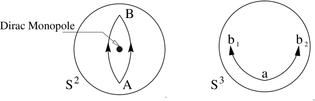
FIG. 1.: Transport of a vector on $S^{2}$ defines transport of a spinor on $S^{3}$. The final spinor state, i.e. the final point on $S^{3}$ depends not only the final point of on $S^{2}$ but on the path itself. Points $b_{1}$ and $b_{2}$ on $S^{3}$ have the same image B on $S^{2}$ under the first Hopf map.

The transport of $z_{\alpha}$ is uniquely defined by the non-singular gauge potential $\Omega$. Since the two points $b_{1}$ and $b_{2}$ differ from each other by a pure phase, they are projected to the same point $B$ on $S^{2}$. Their phase difference is exactly the Berry’s phase. Since $S^{3}$ is locally isomorphic to $S^{2}\times U(1)$, it encapsulates the full quantum information, including both the direction of the $SO(3)$ vector and the phase of the $SO(3)$ spinor. This way, we can also understand the singularity associated with a Dirac monopole as arising from the projection from a non-singular $U(1)$ gauge field on $S^{3}$.

There is an elegant generalization from these considerations to the case of a $SO(5)$ spinor. The $SU(2)$ holonomy of a $SO(5)$ spinor and the Yang monopole are deeply related to the second Hopf map from $S^{7}$ to $S^{4}$ and a non-commutative division algebra called quaternions. A quaternion with three imaginary units ${\bf i}$, ${\bf j}$ and ${\bf k}$ is a generalization of a complex number with one imaginary unit $i$. These three imaginary units mutually anticommute and they obey the following multiplication table:

$${\bf i}^{2}={\bf j}^{2}={\bf k}^{2}=-1\ \ ;\ \ {\bf i}{\bf j}={\bf k}\ \ ;\ \ {\bf j}{\bf k}={\bf i}\ \ ;\ \ {\bf k}{\bf i}={\bf j}$$ (91)

It is simple to understand quaternions from a physicist’s view point, since the algebra of these three imaginary units ${\bf\Sigma}^{\lambda}=({\bf i,j,k})$ is identical to the algebra of three Pauli matrices $\sigma^{\lambda}$, and a one-to-one correspondence between them is therefore possible. A quaternion can be expressed as

$${\bf q}=q^{0}+q^{1}~{}{\bf i}+q^{2}~{}{\bf j}+q^{3}~{}{\bf k}$$ (92)

and therefore has four real components. Complex conjugation of quaternions is defined as the operation that changes the sign of the imaginary parts, i.e. of the last three components. Magnitude of the quaternion is given by $|{\bf q}|^{2}={\bf q}^{*}{\bf q}$. Using a two component quaternion, we can parameterize the $S^{7}$ sphere by

$${\bf q}_{\alpha}=\left(\begin{array}[]{c}{\bf q}_{1}\\ {\bf q}_{2}\end{array}\right)\ \ ;\ \ {\bf q}^{\dagger}{\bf q}=|{\bf q}_{1}|^{2}+|{\bf q}_{2}|^{2}=1$$ (95)

With this notation, the second Hopf map can be expressed as a simple generalization of (88):

$$\eta_{2}:~{}n_{a}={\bf q}^{\dagger}\gamma_{a}{\bf q}$$ (96)

Here $n_{a}$ is a five dimensional real vector, and the five $2\times 2$ quaternionic valued $\gamma$ matrices are defined as a simple generalization of the Pauli matrices

$$\gamma_{1}=\left(\begin{array}[]{cc}0&1\\ 1&0\end{array}\right)\hskip 28.45274pt\gamma_{2}=\left(\begin{array}[]{cc}0&-{\bf i}\\ {\bf i}&0\end{array}\right)\hskip 28.45274pt\gamma_{3}=\left(\begin{array}[]{cc}0&-{\bf j}\\ {\bf j}&0\end{array}\right)$$ (103)

$$\gamma_{4}=\left(\begin{array}[]{cc}0&-{\bf k}\\ {\bf k}&0\end{array}\right)\hskip 28.45274pt\gamma_{5}=\left(\begin{array}[]{cc}1&0\\ 0&-1\end{array}\right)\hskip 106.69783pt$$ (108)

From the norm of ${\bf q}_{\alpha}$ defined in (95) and the properties of the $\gamma$ matrices, one can easily show that $n_{a}^{2}=1$. Therefore, (96) defines a mapping from $S^{7}$ to $S^{4}$. It may be compared with Section II A where an $SO(5)$ spinor was represented by a four component complex vector $\Psi_{\alpha}$ and equation (15) implied that each spinor was mapped into an $SO(5)$ vector by

$$n_{a}=\Psi^{\dagger}\Gamma_{a}\Psi$$ (109)

Connection between two representations is easily established by choosing

$$\Psi^{T}=\{{q}_{2}^{1}+i{q}_{2}^{2},{q}_{1}^{1}+i{q}_{1}^{2},{q}_{2}^{0}-i{q}_{2}^{3},{q}_{1}^{0}-i{q}_{1}^{3}\}$$ (110)

which makes (96) and (109) identical, and turns the second equation in (95) into a normalization condition for the spinor wavefunction.

Any $SU(2)$ gauge field ${\cal A}$ can be expressed in terms of the Pauli matrices as ${\cal A}^{a}={\cal A}^{a\lambda}\sigma_{\lambda}$. Because of the isomorphism between the Pauli matrices $\sigma^{\lambda}$ and the three imaginary quaternionic units ${\bf\Sigma}^{\lambda}=({\bf i,j,k})$, a $SU(2)$ gauge field can also be expressed as a imaginary quaternionic field:

$$i~{}{\bf A}^{a}=A^{\lambda a}{\bf\Sigma}_{\lambda}$$ (111)

Using this observation and directly substituting the definition of the second Hopf map (96) into the $SU(2)$ gauge field of a Yang monopole (46), one finds that it induces a $SU(2)$ gauge field on $S^{7}$ defined by

$${\bf\omega}=i{\cal A}^{a}dn_{a}={\bf\omega}^{\dagger}_{\alpha}d{\bf q}_{\alpha}+{\bf\omega}_{\alpha}d{\bf q}^{\dagger}_{\alpha}=-\frac{1}{2|{\bf q}_{1}|^{2}}[{\bf q}_{1}({\bf q}_{2}^{\dagger}d{\bf q}_{2}-d{\bf q}^{\dagger}_{2}{\bf q}_{2}){\bf q}^{\dagger}_{1}-|{\bf q}_{2}|^{2}(d{\bf q}_{1}{\bf q}_{1}^{\dagger}-{\bf q}_{1}d{\bf q}^{\dagger}_{1})]$$ (112)

where we established correspondence between quaternions and Pauli matrices as

$${\bf i}\rightarrow i\sigma_{y}\hskip 28.45274pt{\bf j}\rightarrow-i\sigma_{x}\hskip 28.45274pt{\bf k}\rightarrow-i\sigma_{z}$$ (113)

The $SU(2)$ gauge field in (112) is singular on a three dimensional “great sphere” $|{\bf q}_{1}|=0$ of $S^{7}$. Fortunately, just like the case of the first Hopf map, the singularity can be completely removed by a $SU(2)$ gauge transformation defined by a unitary quaternion ${\bf u}={\bf q}_{1}/|{\bf q}_{1}|$. The resulting $SU(2)$ gauge field

$${\bf\Omega}={\bf u}^{-1}{\bf\omega}{\bf u}+{\bf u}^{-1}d{\bf u}=-\frac{1}{2}~{}({\bf q}_{\alpha}^{\dagger}d{\bf q}_{\alpha}-d{\bf q}^{\dagger}_{\alpha}{\bf q}_{\alpha})$$ (114)

This $SU(2)$ gauge field over $S^{7}$ appears as a direct quaternionic generalization of the $U(1)$ gauge field over $S^{3}$, and it is non-singular everywhere. Similarly, one can map the singular $SU(2)$ gauge field $\tilde{\cal A}_{+}$ on $S^{3}$ to a singular $SU(2)$ gauge field $\tilde{\bf\omega}$ on $S^{7}$. Upon removing the singularity by a unitary quaternion ${\tilde{\bf u}}={\bf q}_{2}/|{\bf q}_{2}|$, the resulting $SU(2)$ gauge field is again given by the non-singular gauge field ${\bf\Omega}$.

Like the previous calculation, this calculation demonstrates the deep relation between the second Hopf map, Yang’s monopole and the $SU(2)$ holonomy of a $SO(5)$ spinor. We can think of the second Hopf map as defining a relation between a $SO(5)$ vector $n_{a}$ and a normalized $SO(5)$ spinor ${\bf q}_{\alpha}=({\bf q}_{1},{\bf q}_{2})$. This relation is invariant under a quaternionic unitary transformation ${\bf q}_{\alpha}\rightarrow{\bf q}_{\alpha}{\bf u}$ with ${\bf u}^{\dagger}{\bf u}=1$. Such a quaternionic unitary transformation is identical to a $SU(2)$ gauge transformation. In this case, if the $n_{a}$ vector goes from point $A$ to point $B$ on $S^{4}$ via two different paths, the ${\bf q}_{\alpha}$ vector is transported from point $a$ to two different points $b_{1}$ and $b_{2}$ on $S^{7}$. (See figure 2).

FIG. 2.: When a vector is transported on $S^{4}$ along two different paths a spinor is transported on $S^{7}$ to two different final states $b_{1}$ and $b_{2}$, which have the same image B on $S^{4}$.

The transport of ${\bf q}_{\alpha}$ is uniquely defined by the non-singular gauge potential ${\bf\Omega}$. Since the two points $b_{1}$ and $b_{2}$ differ from each other by a $SU(2)$ gauge transformation, they are projected to the same point $B$ on $S^{4}$. Their difference is exactly the $SU(2)$ holonomy of a $SO(5)$ spinor. Since $S^{7}$ is locally isomorphic to $S^{4}\times SU(2)$, it encapsulates the full quantum information, including both the direction of the $SO(5)$ vector and the $SU(2)$ holonomy of a $SO(5)$ spinor.

Another way of seeing the invariance of the second Hopf map under $SU(2)$ gauge transformation comes from returning to a representation of the $SO(5)$ spinor as a four component complex vector $\Psi$. Choosing components of $\Psi$ as

$$\Psi=\{\psi_{1},\phi_{1},\psi_{2}^{\dagger},\phi_{2}^{\dagger}\}^{T}$$ (115)

gives for the second Hopf map $n_{a}=\Psi^{\dagger}\Gamma_{a}\Psi$

$$n_{1} = \phi^{\dagger}_{\alpha}\psi_{\alpha}+\psi^{\dagger}_{\alpha}\phi_{\alpha}$$ (116)

$$n_{2} = i(\phi^{\dagger}_{\alpha}\psi_{\alpha}-\psi^{\dagger}_{\alpha}\phi_{\alpha})$$ (117)

$$n_{3} = \epsilon_{\alpha\beta}(\phi_{\alpha}\psi_{\beta}+\psi^{\dagger}_{\alpha}\phi_{\beta}^{\dagger})$$ (118)

$$n_{4} = i\epsilon_{\alpha\beta}(\phi_{\alpha}\psi_{\beta}-\psi^{\dagger}_{\alpha}\phi_{\beta}^{\dagger})$$ (119)

$$n_{5} = \phi^{\dagger}_{\alpha}\phi_{\alpha}-\psi^{\dagger}_{\alpha}\psi_{\alpha}$$ (120)

One can easily see that this exhausts all possible bilinear combinations that are both real and invariant under simultaneous $SU(2)$ rotations of $\phi$ and $\psi$ [28].

To conclude this section we remark that analysis presented here leads us to an intriguing conclusion that not all spheres are created equal. $S^{3}$ and $S^{7}$ are endowed with a unique algebraic structure and associated non-singular complex (90) and quaternionic (114) gauge connections. This deep connection between the algebra and geometry underlies the non-trivial holonomy of $SO(3)$ and $SO(5)$ spinors.

E $HP(1)$ Representation of the SO(5) Nonlinear $\sigma$ Model

It has long been known that the $SO(3)$ nonlinear sigma model used to describe the low energy physics of magnetic systems has an interesting representation due to the existence of the first Hopf map: $CP(1)$ representation [29]. Indeed one observes that when we define the first Hopf map as in equations (87) and (88) of Section II D, the partition function for the nonlinear sigma model may be written as a path integral over $z$ and gauge field $A$

$$Z=\int{\cal D}ne^{-\int_{0}^{\beta}d\tau\int d^{d}x\frac{1}{4}(\partial_{\mu}n^{a})^{2}}=\int{\cal D}A{\cal D}ze^{-\int_{0}^{\beta}d\tau\int d^{d}x~{}|(\partial_{\mu}-iA_{\mu})z|^{2}}$$ (121)

This may be easily proven by noticing that the action on the right hand side of (121) is quadratic in $A$, so integration over the gauge field amounts to taking the saddle point value

$$A_{\mu}=-\frac{i}{2}\left[z^{\dagger}\partial_{\mu}z-(\partial_{\mu}z^{\dagger})z\right]$$ (122)

After that simple algebra gives

$$\frac{1}{4}(\partial_{\mu}n^{a})^{2}=|(\partial_{\mu}-iA_{\mu})z|^{2}$$ (123)

which proves equation (121). Notice that the gauge field in (122) is the same as in (90), which is not surprising since the origin of both gauge fields is the invariance of (88) and (123) under gauge transformations

$$z_{i} \rightarrow e^{i\phi}z_{i}$$ (124)

$$A_{\mu} \rightarrow A_{\mu}+\partial_{\mu}\phi$$ (125)

Analogously one can prove that the second Hopf map, defined by (95) and (96) in Section II D, gives rise to an $HP(1)$ representation of the $SO(5)$ nonlinear sigma model

$$Z=\int{\cal D}ne^{-\int_{0}^{\beta}d\tau\int d^{d}x\frac{1}{4}(\partial_{\mu}n^{a})^{2}} = \int{\cal D}{\bf B}{\cal D}{\bf q}e^{-\int_{0}^{\beta}d\tau\int d^{d}x~{}(D_{\mu}{\bf q})^{\dagger}(D_{\mu}{\bf q})}$$ (126)

$$D_{\mu}{\bf q} = \partial_{\mu}{\bf q}-{\bf q}{\bf B}_{\mu}$$ (127)

where similarly to $CP(1)$, the $HP(1)$ action

$$\frac{1}{4}(\partial_{\mu}n^{a})^{2}=(D_{\mu}{\bf q})^{\dagger}(D_{\mu}{\bf q})$$ (128)

as well as the second Hopf map (96) are invariant under gauge transformation

$${\bf q}_{\alpha} \rightarrow {\bf q}_{\alpha}{\bf u}$$ (129)

$${\bf B}_{\mu} \rightarrow {\bf u}^{-1}{\bf B}_{\mu}{\bf u}+{\bf u}^{-1}\partial_{\mu}{\bf u}$$ (130)

with ${\bf u}$ being any quaternion that satisfies ${\bf u}^{\dagger}{\bf u}=1$. There is, however, an important difference between gauge transformations in (130) and (125). In the former case they are non-Abelian $SU(2)$ gauge transformations whereas in the latter case they are Abelian $U(1)$ gauge transformations.

It is also not surprising that the saddle point value of the gauge field ${\bf B}$ in (127) is given by

$${\bf B}_{\mu}=-\frac{1}{2}~{}[~{}{\bf q}_{\alpha}^{\dagger}\partial_{\mu}{\bf q}_{\alpha}-(\partial_{\mu}{\bf q}^{\dagger}_{\alpha})~{}{\bf q}_{\alpha}~{}]$$ (131)

which agrees exactly with expression (114) that we obtained in the study of the $SO(5)$ spinor holonomy (notice that both ${\bf B}$ and the one form ${\bf\Omega}$ in (114) are quaternionic imaginary, or anti-hermitian).

So far the $HP(1)$ model is only an interesting reformulation of the $SO(5)$ nonlinear $\sigma$ model. However, it has the advantage that possible topological terms can be easily identified within this formulation. In $2+1$ dimension, one could add the second Hopf invariant, or the non-Abelian Chern-Simons term

$$\frac{n}{8\pi^{2}}~{}Tr\int d^{3}x~{}\epsilon^{\mu\nu\lambda}\left({\bf B}_{\mu}\partial_{\nu}{\bf B}_{\lambda}-\frac{2}{3}{\bf B}_{\mu}{\bf B}_{\nu}{\bf B}_{\lambda}\right)$$ (132)

to the $HP(1)$ action (127), where $Tr$ implies taking the real part of a quaternion ( in representation where quaternions are $2\times 2$ matrices as in (113), it corresponds to actually taking a trace ). Because the Chern-Simons term changes by

$$\frac{n}{16\pi^{2}}~{}Tr\int d^{3}x~{}\epsilon^{\mu\nu\lambda}\left({\bf u}^{-1}(\partial_{\mu}{\bf u}){\bf u}^{-1}(\partial_{\nu}{\bf u}){\bf u}^{-1}(\partial_{\lambda}{\bf u})\right)$$ (133)

under global gauge transformation (130), the coupling constant $n$ has to be quantized ( for $n=1$ expression in (133) is a winding number of the gauge transformation which is always integer), i.e. only integer values of $n$ are allowed. In $3+1$ dimension, one could add a $\theta$ term,

$$\theta Tr\int d^{4}x~{}\epsilon^{\mu\nu\lambda\sigma}{\bf F}_{\mu\nu}{\bf F}_{\lambda\sigma}$$ (134)

$${\bf F}_{\mu\nu} = \partial_{\mu}{\bf B}_{\nu}-\partial_{\nu}{\bf B}_{\mu}+[{\bf B}_{\mu},{\bf B}_{\nu}]$$ (135)

to the action $HP(1)$ action (127). In $6+1$ dimensions, Wu and Zee [18] showed that one could also add an Abelian Chern-Simons term for the 3 index gauge field introduced in (58). However, we haven’t yet identified microscopic models which would give rise to these topological terms in the action.

F Wigner - von Neumann Class

The non-trivial holonomy of the quantum mechanical wave functions are intimately related to the degeneracy point of the Hamiltonian. Wigner and von Neumann classified the degeneracy points into three classes according to the generic symmetries of the Hamiltonian. Time-reversal invariant systems without Kramers degeneracy (system of bosons or even number of fermions) belong to the orthogonal class. The generic degeneracy point has co-dimension $2$, i.e. one needs to tune two parameters simultaneously to zero in order to reach a point of degeneracy. Time-reversal breaking system belong to the unitary class, and the degeneracy point has codimension $3$. Berry’s phase of a $SO(3)$ spinor describes the non-trivial holonomy around this point singularity in the $3$ dimensional parameter space, which can be described as a Dirac monopole. Time-reversal invariant system with Kramers degeneracy (e.g. system with odd number of fermions) belong to symplectic class. The degeneracy point for this class has codimension $5$. Unlike the two previous classes, we have to consider a $4\times 4$ matrix problem in this case, in order to describe the level crossings of two different Kramers doublets. In his seminal work on random matrix theory, Dyson [30] noticed that this situation can be best described as a $2\times 2$ quaternionic matrix problem. In a thorough analysis, Avron et al [19, 20] showed that the natural symmetry for the symplectic class is therefore a unitary rotation of a two component quaternion, which is isomorphic to a $SO(5)$ symmetry group. The non-trivial holonomy of a $SO(5)$ spinor arises when one encircles this degeneracy point in $5$ dimensional space, which acts as a Yang monopole.

In this context, it is highly remarkable that $SO(5)$ symmetry emerges naturally in a generic fermionic system with time reversal symmetry. To make the above discussion more explicit, let us recall that close to the degeneracy point, a generic Hamiltonian without Kramers degeneracy can be expressed as a $2\times 2$ Hermitian matrix

$${\cal H}=\left(\begin{array}[]{cc}a&d\\ c&b\end{array}\right)\hskip 56.9055pta,b\in{\cal R},~{}d^{*}=c\in{\cal C}$$ (138)

whose eigenvalues are

$$\lambda_{\pm}=\frac{a+b\pm\sqrt{(a+b)^{2}-4(ab-|d|^{2})}}{2}$$ (139)

Degeneracy requires $(a-b)^{2}+4|d|^{2}=0$, which is only satisfied when $a=b$ and $Re~{}d=Im~{}d=0$. When the Hamiltonian is real ( for systems without time-reversal symmetry breaking ) we have only two conditions for the degeneracy point, i.e. the co-dimension is $2$. But when the time reversal-breaking is present, we have three conditions and the codimension is $3$.

Up to a overall additive constant, this $2\times 2$ Hamiltonian can be mapped onto a effective spin $1/2$ problem in a magnetic field: ${\cal H}_{\alpha\beta}=n_{a}\sigma^{a}_{\alpha\beta}$, where $n_{a}$ labels the three directions away from the degeneracy point $n_{a}=0$. Wave functions defined for parameters on $S^{2}$ enclosing the singularity are non-degenerate, but experience non-trivial holonomy due to the degeneracy point, as discussed in Section II A.

Close to the degeneracy point of two Kramers doublets, the Hamiltonian is a $4\times 4$ matrix, and can be represented by the matrix of a spin $3/2$ particle. However, because of the time reversal symmetry, the Hamiltonian has to be quadratic in these spin $3/2$ matrices. Avron et al [19, 20] showed that a generic Hamiltonian close to the degeneracy point can be expressed as

$${\cal H}_{\alpha\beta}=\sum_{i,j}Q_{ij}S^{i}_{\alpha\gamma}S^{j}_{\gamma\beta}$$ (140)

where $S^{i}_{\alpha\gamma}$ are the three $4\times 4$ spin $3/2$ matrices, and $Q_{ij}$ is a $3\times 3$ real symmetric traceless matrix. Since $Q_{ij}$ has $5$ real entries, and one needs to tune all of them to zero to get a degeneracy of two Kramers doublets, therefore the codimension of the degeneracy point is $5$. In fact, this is nothing but a quadrupole spin Hamiltonian first used by Zee [31] and other authors[32, 33] to illustrate the concept of non-Abelian holonomy.

This generic Hamiltonian for the symplectic class (140) has a hidden $SO(5)$ symmetry. Since $Q_{ij}$ has exactly five entries, we can choose a orthonormal basis set $Q^{a}_{ij}$, $(a=1,..5)$ satisfying $Tr(Q^{a}Q^{b})=\frac{2}{3}\delta^{ab}$ and expand $Q_{ij}$ as $Q_{ij}=\sum_{a}n_{a}Q^{a}_{ij}$. In this representation, the generic Hamiltonian (140) can be expressed as

$${\cal H}_{\alpha\beta}=n_{a}\Gamma^{a}_{\alpha\beta}\ \ ;\ \ \Gamma^{a}_{\alpha\beta}=S^{i}_{\alpha\gamma}Q^{a}_{ij}S^{j}_{\gamma\beta}$$ (141)

At this point, the hidden $SO(5)$ symmetry becomes manifest. Since the five $\Gamma$ matrices obey a $SO(5)$ Clifford algebra, this Hamiltonian is identical to the $SO(5)$ spinor Hamiltonian (15) discussed in section II A.

Therefore, we see that $SO(5)$ symmetry arises naturally close to any generic degeneracy point of a time reversal invariant Hamiltonian with Kramers degeneracy. Both AF and dSC states in the high $T_{c}$ problem are time reversal invariant, and their quasi-particle states form degenerate pairs. At the fermi liquid point, two of these pairs become additionally degenerate. Therefore $SO(5)$ symmetry emerges naturally in this system. The non-Abelian holonomy of the SDW and BCS quasi-particles arises close to the fermi liquid degeneracy point, which is identified with a Yang monopole in the parameter space.

III Effective Adiabatic Action for the SO(5) Non-Linear $\sigma$ Model

A Effective Action Arising from Berry’s Phase

Let us now consider the problem of a rigid $SO(5)$ rotor interacting with a $SO(5)$ spinor. We want to integrate out the spinor degrees of freedom and ask whether this procedure will generate any additional contributions to the action for the $SO(5)$ rotator ( see Kuratsuji and Iida [34] and M. Stone [24] for such discussion in the case of coupled $SO(3)$ spinor and rotor ).

Our system is described by the Hamiltonian

$${\cal H} = {\cal H}_{0}+{\cal H}_{I}$$ (142)

$${\cal H}_{0} = \frac{1}{2I}\sum_{a<b}L_{ab}^{2}$$ (143)

Here ${\cal H}_{0}$ is the usual action of the $SO(5)$ rigid rotor [1] with $L_{ab}$ being the generators of rotation, and ${\cal H}_{I}$ is the Hamiltonian (15). The states of this composite system are defined as product states

$$|\Psi_{\alpha}[n],n_{a}\rangle=|\Psi_{\alpha}[n]\rangle\otimes|n_{a}\rangle$$ (144)

where $|n_{a}\rangle$ are the states of the $SO(5)$ vector and $|\Psi_{\alpha}[n]\rangle$ are spinor states. We choose $|\Psi_{\alpha}[n]\rangle$ to be eigenstates of ${\cal H}_{I}(n,\Psi)$, i.e. they diagonalize (143) for a given orientation of $n_{a}$.

$${\cal H}_{I}(n,\Psi)|\Psi_{\alpha}[n]\rangle=E_{\alpha}|\Psi_{\alpha}[n]\rangle$$ (145)

The partition function is defined as

$$Z(\beta)=\sum_{n,\alpha}\langle\Psi_{\alpha}[n(0)],n_{a}(0)|e^{-\beta{\cal H}}||\Psi_{\alpha}[n(0)],n_{a}(0)\rangle$$ (146)

with summation going over all states of $n_{a}$ and $\Psi_{\alpha}$. Let us perform time discretization and insert resolution of identity for the $n$-states. We make $N$ intervals of length $\epsilon$ with $N\epsilon=\beta$:

$$Z(\beta)=\prod_{k=1}^{N-1}\int d\mu(n_{k})\sum_{n(0),\alpha}\langle\Psi_{\alpha}[n(0)],n_{a}(0)|e^{-{\cal H}\epsilon}|n(N-1)\rangle\langle n(N-1)|\dots|\Psi_{\alpha}[n(0)],n_{a}(0)\rangle$$ (147)

where $d\mu(n_{k})$ is an invariant measure of integration for the $|n_{a}\rangle$ states at interval $k$. When $\epsilon$ is small we have

$$\langle n(k)|e^{-{\cal H}\epsilon}|n(k-1)\rangle=\langle n(k)|e^{-{\cal H}_{0}\epsilon}|n(k-1)\rangle e^{-{\cal H}_{I}(n(k))\epsilon}$$ (148)

and

$$Z(\beta)= \sum_{n(0),\alpha}\langle n(0)|e^{-{\cal H}_{0}\epsilon}|n(N-1)\rangle\langle n(N-1)|e^{-{\cal H}_{0}\epsilon}|n(N-2)\rangle\dots\langle n(1)|e^{-{\cal H}_{0}\epsilon}|n(0)\rangle\times$$ (149)

$$\times \langle\Psi_{\alpha}[n(0)]|e^{-{\cal H}_{I}(n_{N})\epsilon}e^{-{\cal H}_{I}(n_{N-1})\epsilon}\dots e^{-{\cal H}_{I}(n_{1})\epsilon}|\Psi_{\alpha}[n(0)]\rangle$$ (150)

The first line of the last equation is clearly the partition function of the $SO(5)$ rotor. Following Auerbach [35] we can write it as

$$\langle n(k)|e^{-{\cal H}_{0}\epsilon}|n(k-1)\rangle=$$ (151)

$$= \int d\mu(p_{k})\langle n(k)|p(k)\rangle\langle p(k)|e^{-{\cal H}_{0}\epsilon}|n(k-1)\rangle$$ (152)

$$= \int d\mu(p_{k})~{}exp\{ip_{a,k}(n_{a,k}-n_{a,k-1})-\frac{1}{2I}\sum_{a<b}(p_{a}n_{b}-p_{b}n_{a})^{2}\epsilon\}$$ (153)

$$= const\times exp\{-\frac{(n_{a}(k)-n_{a}(k-1))^{2}}{2I\epsilon^{2}}\epsilon\}$$ (154)

In the second line of equation (150) we insert the resolution of identity at each $\tau$ step $\sum_{\beta_{j}}|\Psi_{\beta_{j}}[n_{j}]\rangle\langle\Psi_{\beta_{j}}[n_{j}]|=1$, then

$$T_{n\alpha;n\alpha}=\langle\Psi_{\alpha}[n(0)]|e^{-h(n_{N})\epsilon}e^{-h(n_{N-1})\epsilon}\dots e^{-h(n_{1})\epsilon}|\Psi_{\alpha}[n(0)]\rangle=$$ (155)

$$\prod_{j=1}^{N-1}\sum_{\beta_{j}}\langle\Psi_{\alpha}[n(0)]|e^{-h(n_{N})}|\Psi_{b_{N-1}}[n_{N-1}]\rangle\langle\Psi_{b_{N-1}}[n_{N-1}]|\dots|\Psi_{\alpha}[n(0)]\rangle$$ (156)

We now recall the adiabatic hypothesis and realize that in summation over intermediate spinor states in the last expression we only have to consider two states of the same energy as the initial state ( recall discussion of double degeneracy of spinor states in section II A ). In the limit $\epsilon\rightarrow 0$ the last expression becomes the path ordered exponential

$$T_{n\alpha;n\alpha}=e^{-\beta E_{\alpha}}\left(T_{\tau}exp\{i~{}\oint{\cal A}^{a}[n(\tau)]dn_{a}\}\right)_{\alpha\alpha}$$ (157)

Here

$${\cal A}^{a}_{\alpha\beta}[n(t)]=\frac{1}{i}\langle\Psi_{\alpha}[n]|\frac{\partial}{\partial n_{a}}|\Psi_{\beta}[n]\rangle$$ (158)

and indices $\alpha$, $\beta$ take two values that correspond to the two degenerate states of the same energy as the initial state, but with the new orientation of the $n$-field ( new instantaneous eigenstates in the language of section II A ). Therefore we arrive at the same $SU(2)$ gauge connection ${\cal A}^{a}$ as defined in equations (35) and (35). By combining equations (150) and (157) we see that this gauge field ${\cal A}^{a}$ defines a non-trivial non-Abelian topological term in the action for the $SO(5)$ rotor

$$Z(\beta)=\int{\cal D}n_{\tau}Tr\left[exp\left\{-\oint_{0}^{\beta}\left(\frac{dn_{a}}{d\tau}\right)^{2}d\tau+i\oint{\cal A}^{a}[n(\tau)]dn_{a}\right\}\right]$$ (159)

In Chapter II D we saw how the first term in this path integral may be written using two quaternions ${\bf q}=({\bf q}_{1},{\bf q}_{2})^{T}$

$$\frac{1}{4}\left(\frac{dn_{a}}{d\tau}\right)^{2}=({\cal D}_{\tau}{\bf q})^{\dagger}({\cal D}_{\tau}{\bf q})$$ (160)

$${\cal D}_{\tau}{\bf q}=~{}\partial_{\tau}{\bf q}-{\bf q}{\bf B}({\tau})\hskip 14.22636pt \hskip 14.22636pt{\bf B}(\tau)=-\frac{1}{2}\left[{\bf q}_{\alpha}^{\dagger}\partial_{\tau}{\bf q}_{\alpha}-(\partial_{\tau}{\bf q}_{\alpha}^{\dagger}){\bf q}_{\alpha}\right]$$ (161)

As it turns out, the second term of equation (159) can also be represented using quaternions

$$i{\cal A}^{a}[n(\tau)]dn_{a}\rightarrow{\bf q}_{\alpha}^{\dagger}\partial_{\tau}{\bf q}_{\alpha}d\tau=-{\bf B}({\tau})d\tau$$ (162)

Therefore, the $HP(1)$ representation of (159) reads:

$$Z(\beta)=\int{\cal D}{\bf B}{\cal D}{\bf q}~{}Tr\left[exp\left\{-\int_{0}^{\beta}d\tau~{}\left((D_{\tau}{\bf q})^{\dagger}(D_{\tau}{\bf q})+{\bf B}({\tau})\right)\right\}\right]$$ (163)

IV Physical Interpretation of the SU(2) Holonomy

A Holonomy on a Rung in the $SO(5)$ Ladder Problem

Having established the necessary mathematical framework, we are now in a position to discuss the physical application to the holonomy between SDW and BCS quasi-particles. As a warm-up exercise, let us first consider a two site problem ( see Figure 3).

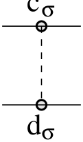
FIG. 3.: Two site problem. Electrons on the upper site of the of the rung are created by $c_{\sigma}^{\dagger}$ operators and $d_{\sigma}^{\dagger}$ creates electrons on the lower site.

Recently, Scalapino, Hanke and one of us (SCZ)[7] studied a $SO(5)$ symmetric ladder model, and classified the $SO(5)$ operator content for the two site problem. They introduced a $SO(5)$ spinor

$$\Psi_{\alpha}=\left(\begin{array}[]{c}c_{\sigma}\\ d^{\dagger}_{\sigma}\end{array}\right)$$ (166)

where $c_{\sigma}^{\dagger}$ and $d_{\sigma}^{\dagger}$ operators create electrons on the upper and lower sites of the rung respectively. If we consider the $SO(5)$ vector interaction on the same rung, and introduce a time-dependent Hubbard-Stratonovich field $n_{a}(t)$ to decouple the interaction, we obtain the following effective fermion problem on a rung:

$${\cal H}(t)=\Delta~{}n_{a}(t)\Psi^{\dagger}_{\alpha}\Gamma^{a}_{\alpha\beta}\Psi_{\beta}$$ (167)

Our task is to find the ground state and low energy quasi-particle excitations for this problem and demonstrate the physical interpretation of the non-Abelian holonomy.

This physical problem is identical to the mathematical problem we posed in section II C. We can transform the problem into the “rotating frame” by decomposing $\Psi_{\alpha}$ according to (61), with a $S_{\alpha\beta}$ matrix satisfying (64) and (65). The resulting Hamiltonian (63) in the “rotating frame” is time independent and diagonal in the $\Phi_{\alpha}$ variable. $\Phi_{1}$ and $\Phi_{3}$ have positive energy, while $\Phi_{2}$ and $\Phi_{4}$ have negative energy. According to the Dirac prescription, we fill the negative energy states and obtain the ground state $|\Omega\rangle$ in the rotating frame:

$$\Phi^{\dagger}_{2}|\Omega\rangle=\Phi^{\dagger}_{4}|\Omega\rangle=0\ \ ;\ \ \Phi_{1}|\Omega\rangle=\Phi_{3}|\Omega\rangle=0$$ (168)

(Notice that the definition of $|\Omega\rangle$ is different from reference [7]). The corresponding elementary excitations are given by

$$\Phi^{\dagger}_{1}|\Omega\rangle\ \ ;\ \ \Phi^{\dagger}_{3}|\Omega\rangle\ \ ;\ \ \Phi_{2}|\Omega\rangle\ \ ;\ \ \Phi_{4}|\Omega\rangle$$ (169)

with degenerate energy $+\Delta$. If the $n_{a}$ vector points to $n_{4}$ direction at $t=0$, the ground state and four elementary excitations can be explicitly expressed in terms of electron operators $c_{\sigma}$ and $d_{\sigma}$, and they are depicted in Figure 4.

FIG. 4.: Ground state and single particle excited states on a rung, when $n_{a}$ points in $n_{4}$ direction.

Within the adiabatic approximation, the $S_{\alpha\beta}$ matrix is explicitly given by (83). The instantaneous ground state and elementary excitations in the original frame is simply obtained from (168) and (169) by substituting $\Phi_{\alpha}=S^{\dagger}_{\alpha\beta}\Psi_{\beta}$. Let us now imagine taking a path of $n_{a}(t)$ on $S^{4}$ which starts and returns to $n_{4}$. Because of the non-Abelian holonomy discussed in section II C, the $S_{\alpha\beta}$ matrix only returns to itself up to a $SU(2)$ transformation in the $(1,3)$ and $(2,4)$ subspaces. In particular, there exist cyclic paths on $S^{4}$ for which

$$S(t=0)=\left(\begin{array}[]{cccc}1&0&0&0\\ 0&1&0&0\\ 0&0&1&0\\ 0&0&0&1\end{array}\right)\ \ ;\ \ S(t=T)=\left(\begin{array}[]{cccc}0&0&1&0\\ 0&0&0&1\\ 1&0&0&0\\ 0&1&0&0\end{array}\right)$$ (178)

Under such a cyclic path, the quasi-particle state $\Psi^{\dagger}_{1}|\Omega\rangle$ interchanges with $\Psi^{\dagger}_{3}|\Omega\rangle$, while the quasi-particle state $\Psi_{2}|\Omega\rangle$ interchanges with $\Psi_{4}|\Omega\rangle$ ( see Figure 5).

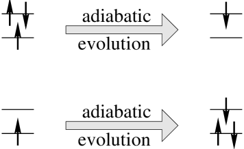
FIG. 5.: Interchange of degenerate spinor states after cyclic adiabatic rotation of the superspin.

Therefore, we obtained a simple physical interpretation of the $SU(2)$ non-Abelian holonomy in terms of interchange of certain degenerate pairs of quasi-particle states on a rung. It is important to notice that the degeneracy of these pairs is generic in any model with spin rotation and charge conjugation symmetry, and does not require any special fine tuning of parameters that is required to render the model $SO(5)$ symmetric in all sectors[7]. For this reason, we believe that the non-Abelian holonomy we discussed in this work have general applicability beyond exactly $SO(5)$ symmetric models.

We notice that in the course of a cyclic adiabatic evolution, a SDW quasi-particle can be turned into a SDW quasi-hole (see Figure 5). In this sense, this phenomenon is very analogous to Andreev reflection at the metal/superconductor interfaces, where a metallic quasi-particle reflects back as a quasi-hole, and emits a Cooper pair into the superconductor. However, close inspection of the spin quantum numbers shows that a $\pi$ pair [1, 2], rather than a Cooper pair is emitted in our problem. Indeed, the states interchanged after cyclic adiabatic transport of the superspin differ from each other by addition/removal of a pair of electrons in a triplet state ( a pair of spin up electrons for the first pair of degenerate states on figure 5, and a pair of spin down electrons for the second pair of degenerate states on figure 5 ). Operators that create such triplet pairs are generators of the $SO(5)$ symmetry on the rung [7] ($\pi$ operators), they carry charge $2$ and spin $1$. By contrast, the operator that produces a $d$-wave Cooper pair creates two electrons on opposite sites in a singlet state, therefore it carries charge 2 and spin 0.

The appearance of the $\pi$ operators as operators of the holonomy is not surprising and is related to the symmetry content of Hamiltonian (167). For a fixed direction of $n_{a}$ the symmetry of this Hamiltonian is reduced from $SO(5)$ to $SO(4)$. For example when $n_{a}$ points toward $n_{4}$, the $SO(4)$ algebra that commutes with the Hamiltonian is formed by operators that rotate between $n_{1}$, $n_{2}$, $n_{3}$, and $n_{5}$ but leave $n_{4}$ invariant. Let $L_{ab}$ be the operators that rotate between $n_{a}$ and $n_{b}$ ( microscopically, such operators are given by $L_{ab}=\Psi^{\dagger}_{\alpha}\Gamma^{ab}_{\alpha\beta}\Psi_{\beta}$, where $\Gamma^{ab}=i[\Gamma^{a},\Gamma^{b}]$, see [36, 7] for details ), then the generators of the unbroken $SO(4)$ symmetries are

$$K_{1}=\frac{1}{2}~{}(L_{21}-L_{35}) \hskip 28.45274ptK_{2}=\frac{1}{2}~{}(L_{13}-L_{25}) \hskip 28.45274ptK_{3}=\frac{1}{2}~{}(L_{32}-L_{15})$$ (179)

$$J_{1}=\frac{1}{2}~{}(L_{21}+L_{35}) \hskip 28.45274ptJ_{2}=\frac{1}{2}~{}(L_{13}+L_{25}) \hskip 28.45274ptJ_{3}=\frac{1}{2}~{}(L_{32}+L_{15})$$ (180)

$$\left[K_{i},K_{j}\right]=i~{}\epsilon_{ijk}K_{k} \hskip 28.45274pt\left[J_{i},K_{j}\right]=0 \hskip 28.45274pt\left[J_{i},J_{j}\right]=i~{}\epsilon_{ijk}J_{k}$$ (181)

We have chosen the generators in a form that makes transparent a property of $SO(4)$ to be factorizable into $SU(2)\times SU(2)$. The eigenstates of our Hamiltonian have to form multiplets that transform as irreducible representations of this unbroken $SO(4)$. But $SO(4)$ multiplets also factorize into products of $SU(2)$ multiplets, and by acting with operator $K_{+}=\pi^{\dagger}_{x}-i\pi^{\dagger}_{y}=-ic_{\downarrow}^{\dagger}d_{\downarrow}^{\dagger}$ or $J_{+}=\pi_{x}-i\pi_{y}=-ic_{\uparrow}d_{\uparrow}$ one can move between states related by holonomy. For example, states $\Phi_{1}^{\dagger}|\Omega\rangle$ and $\Phi_{3}^{\dagger}|\Omega\rangle$ form an $SO(4)$ multiplet that is a doublet of the $J$ algebra and a singlet of the $K$ algebra, whereas the states $\Phi_{2}|\Omega\rangle$ and $\Phi_{3}|\Omega\rangle$ form an $SO(4)$ multiplet that is a doublet of the $K$ algebra and a singlet of the $J$ algebra. Also since the two pairs belong to different multiplets holonomy does not mix them.

B SU(2) Holonomy of BCS and SDW Quasi-particles

Having illustrated the physical interpretation of the $SU(2)$ holonomy in a $2$ site problem, we are now ready to investigate the physical interpretation in terms of SDW and BCS quasi-particles. We start from the tight-binding Hamiltonian with $SO(5)$ symmetric vector interaction. We write it in spinor representation following notations in [36]

$${\cal H}(t)= {\sum_{{\bf p}\alpha}}^{\prime}\epsilon_{\bf p}(\Psi_{{\bf p}\alpha}^{\dagger}\Psi_{{\bf p}\alpha}-\Psi_{{\bf p}+{\bf Q}\alpha}^{\dagger}\Psi_{{\bf p}+{\bf Q}\alpha})$$ (183)

$$\hskip 28.45274pt+~{}{\sum_{{\bf p}\alpha\beta}}^{\prime}\Delta_{\bf p}~{}n^{a}(t)~{}(\Psi_{{\bf p}\alpha}\Gamma^{a}_{\alpha\beta}\Psi_{{\bf p}+{\bf Q}\beta}+\Psi_{{\bf p}+{\bf Q}\alpha}^{\dagger}\Gamma^{a}_{\alpha\beta}\Psi_{{\bf p}\beta})$$

Here

$$\Psi_{{\bf p}}^{T}=\{c_{{\bf p}\uparrow},c_{{\bf p}\downarrow},\phi_{\pi}({\bf p})~{}c^{\dagger}_{-{\bf p}+{\bf Q}\uparrow},\phi_{\pi}({\bf p})~{}c^{\dagger}_{-{\bf p}+{\bf Q}\downarrow}\}$$ (184)

is the $SO(5)$ spinor with $\phi_{\pi}({\bf p})=sgn(cosp_{x}-cosp_{y})$ and prime over ${\sum_{\bf p}}^{\prime}$ denotes summation over half of the Brillouin zone). When $n_{a}$ points in the $2,3,4$ directions, this is nothing but the SDW mean field Hamiltonian. When $n_{a}$ points in the $1,5$ direction, it represents the BCS mean field Hamiltonian. We are interested here in the case where the $n_{a}(t)$ field is time dependent. This situation would arise naturally when one performs a Hubbard Stratonovich decomposition of the interaction term, and $n_{a}(t)$ is a dynamic mean field. As the $n_{a}(t)$ field fluctuates in time, the quasi-particles “rotate” between SDW and BCS characters. Here we would like to consider the adiabatic limit of this fluctuation and identify the associated holonomy between SDW and BCS quasi-particles.

Following the discussions in sections II C, we decompose $\Psi_{{\bf p}\alpha}$ as

$$\Psi_{{\bf p}\alpha}(t)=S_{\alpha\beta}(t)\Phi_{{\bf p}\beta}(t)$$ (185)

where the spinor rotation matrix $S_{\alpha\beta}$ satisfies the same conditions (64) and (65) as before. Substituting this decomposition into (183), we find the Hamiltonian in the “rotating frame”:

$${\cal H}_{0}={\sum_{{\bf p}\alpha}}^{\prime}\epsilon_{\bf p}(\Phi_{{\bf p}\alpha}^{\dagger}\Phi_{{\bf p}\alpha}-\Phi_{{\bf p}+{\bf Q}\alpha}^{\dagger}\Phi_{{\bf p}+{\bf Q}\alpha})+{\sum_{{\bf p}\alpha\beta}}^{\prime}\Delta_{\bf p}~{}(\Phi_{{\bf p}\alpha}^{\dagger}\Gamma^{4}_{\alpha\beta}\Phi_{{\bf p}+{\bf Q}\beta}+\Phi_{{\bf p}+{\bf Q}\alpha}^{\dagger}\Gamma^{4}_{\alpha\beta}\Phi_{{\bf p}\beta})$$ (186)

This Hamiltonian can be easily diagonalized by a $SO(5)$ generalization of the Bogoliubov transformation:

$$\gamma^{c}_{{\bf p}\uparrow} =u_{\bf p}\Phi_{{\bf p}1}+v_{\bf p}\Phi_{{\bf p}+{\bf Q}1}\hskip 28.45274pt\gamma^{v\dagger}_{-{\bf p}\uparrow} =u_{\bf p}\Phi_{{\bf p}3}+v_{\bf p}\Phi_{{\bf p}+{\bf Q}3}$$ (187)

$$\gamma^{c}_{{\bf p}\downarrow} =-u_{\bf p}\Phi_{{\bf p}2}+v_{\bf p}\Phi_{{\bf p}+{\bf Q}2}\hskip 28.45274pt\gamma^{v\dagger}_{-{\bf p}\downarrow} =-u_{\bf p}\Phi_{{\bf p}4}+v_{\bf p}\Phi_{{\bf p}+{\bf Q}4}$$ (188)

$$\gamma^{v}_{{\bf p}\uparrow} =v_{\bf p}\Phi_{{\bf p}1}-u_{\bf p}\Phi_{{\bf p}+{\bf Q}1}\hskip 28.45274pt\gamma^{c\dagger}_{-{\bf p}\uparrow} =v_{\bf p}\Phi_{{\bf p}3}-u_{\bf p}\Phi_{{\bf p}+{\bf Q}3}$$ (189)

$$\gamma^{v}_{{\bf p}\downarrow} =v_{\bf p}\Phi_{{\bf p}2}+u_{\bf p}\Phi_{{\bf p}+{\bf Q}2}\hskip 28.45274pt\gamma^{c\dagger}_{-{\bf p}\downarrow} =v_{\bf p}\Phi_{{\bf p}4}+u_{\bf p}\Phi_{{\bf p}+{\bf Q}4}$$ (190)

where $v_{\bf p}=\sqrt{\frac{1}{2}\left(1-\epsilon_{\bf p}/E_{\bf p}\right)}$,  $u_{\bf p}=\sqrt{\frac{1}{2}\left(1+\epsilon_{\bf p}/E_{\bf p}\right)}$ and $E_{\bf p}=\sqrt{\epsilon^{2}_{\bf p}+\Delta^{2}_{\bf p}}$ . We obtain

$${\cal H}_{0}=\sum_{{\bf p}\sigma}E_{{\bf p}}\left(\gamma^{c\dagger}_{{\bf p}\sigma}\gamma^{c}_{{\bf p}\sigma}-\gamma^{v\dagger}_{{\bf p}\sigma}\gamma^{v}_{{\bf p}\sigma}\right)$$ (191)

and the ground state $|\Omega\rangle$ is obtained by filling the negative energy states:

$$\gamma^{c}_{\pm{\bf p}\sigma}|\Omega\rangle=0\hskip 42.67912pt\gamma^{v\dagger}_{\pm{\bf p}\sigma}|\Omega\rangle=0$$ (192)

Excited states

$$\gamma^{c\dagger}_{\pm{\bf p}\sigma}|\Omega\rangle\hskip 28.45274pt\gamma^{v}_{\pm{\bf p}\sigma}|\Omega\rangle$$ (193)

are degenerate with energy $E_{\bf p}$. If at $t=0$ the superspin $n_{a}$ points towards $n_{4}$, these quasiparticle states are readily expressed in terms of electron creation/annihilation operators

$$\gamma^{c\dagger}_{\pm{\bf p}\sigma}|\Omega\rangle=\left(\sigma~{}u_{\bf p}c^{\dagger}_{\pm{\bf p}\sigma}+v_{\bf p}c^{\dagger}_{\pm{\bf p}+{\bf Q}\sigma}\right)|\Omega\rangle$$ (194)

$$\gamma^{v}_{\pm{\bf p}\sigma}|\Omega\rangle=\left(v_{\bf p}c_{\pm{\bf p}\sigma}-\sigma~{}u_{\bf p}c_{\pm{\bf p}+{\bf Q}\sigma}\right)|\Omega\rangle$$ (195)

Elementary excitations in the original frame are constructed as $\Phi_{{\bf p}\alpha}=S^{\dagger}_{\alpha\beta}(t)\Psi_{{\bf p}\beta}$ where in the adiabatic approximation matrix $S_{\alpha\beta}$ is taken from (83).

Now we imagine that $n_{a}(t)$ makes a closed adiabatic rotation as discussed in section IV A. It starts from $n_{4}$ and returns at $t=T$ to the same direction. However, the matrix $S$ at time $T$ does not have to return to unity and it may come back in the form given in (178). Equation (185) then instantly tells us that after such cyclic rotation of the superspin the quasiparticle state $\gamma^{c\dagger}_{{\bf p}\uparrow}|\Omega\rangle$ interchanges with $\gamma^{v}_{-{\bf p}\uparrow}|\Omega\rangle$, and $\gamma^{c\dagger}_{{\bf p}\downarrow}|\Omega\rangle$ interchanges with $\gamma^{v}_{-{\bf p}\downarrow}|\Omega\rangle$. This means that after superspin completes a revolution, quasiparticle in the conductance band returns as a missing quasiparticle in the valence band with the same spin but opposite momentum. SDW quasiparticle and SDW quasihole have been interchanged! What has been emitted in such process is an object with spin 1 and charge $2$

$$\pi_{{\bf p}\sigma}=\gamma^{c}_{-{\bf p}\sigma}\gamma^{v}_{{\bf p}\sigma}=\phi_{\pi}({\bf p})~{}c_{-{\bf p}+{\bf Q}\sigma}c_{{\bf p}\sigma}+\dots$$ (196)

When summed over all ${\bf p}$’s the terms in $\dots$ disappear and we get one of generators of $SO(5)$ algebra, the $\pi$ operator [1, 2]. So we obtained again that adiabatic transport of the superspin leads to a $SO(5)$ generalization of Andreev reflection, in which a $\pi$ particle has been emitted.

Interpretation of this result using unbroken $SO(4)$ symmetry of Hamiltonian (183) is straightforward. When $n_{a}$ points along $n_{4}$, the important generators of this unbroken symmetry ( see discussion after equation (181) ) are

$$K_{+} = \frac{1}{2}(L_{21}-L_{35}+iL_{13}-iL_{25})$$ (197)

$$= {\sum_{{\bf p}}}\phi_{\pi}({\bf p})c_{{\bf p}\downarrow}^{\dagger}c_{-{\bf p}+{\bf Q}\downarrow}^{\dagger}={\sum_{{\bf p}}}^{\prime}\gamma^{v\dagger}_{{\bf p}\downarrow}\gamma^{c\dagger}_{-{\bf p}\downarrow}$$ (198)

$$J_{+} = \frac{1}{2}(L_{21}+L_{35}+iL_{13}+iL_{25})$$ (199)

$$= {\sum_{\bf p}}\phi_{\pi}({\bf p})c_{-{\bf p}+{\bf Q}\uparrow}c_{-{\bf p}\uparrow}={\sum_{{\bf p}}}^{\prime}\gamma^{c}_{-{\bf p}\uparrow}\gamma^{v}_{{\bf p}\uparrow}$$ (200)

These are $\pi$ operators that move us between pairs of states that form multiplets of the unbroken $SO(4)$.

$$\gamma^{v}_{{\bf p}\downarrow}|\Omega\rangle\stackrel{{\scriptstyle K_{+}}}{{\rightarrow}}\gamma^{c\dagger}_{-{\bf p}\downarrow}|\Omega\rangle$$ (201)

$$\gamma^{v}_{{\bf p}\uparrow}|\Omega\rangle\stackrel{{\scriptstyle J_{-}}}{{\rightarrow}}\gamma^{c\dagger}_{-{\bf p}\uparrow}|\Omega\rangle$$ (202)

$$\gamma^{v}_{-{\bf p}\downarrow}|\Omega\rangle\stackrel{{\scriptstyle K_{+}}}{{\rightarrow}}\gamma^{c\dagger}_{{\bf p}\downarrow}|\Omega\rangle$$ (203)

$$\gamma^{v}_{-{\bf p}\uparrow}|\Omega\rangle\stackrel{{\scriptstyle J_{-}}}{{\rightarrow}}\gamma^{c\dagger}_{{\bf p}\uparrow}|\Omega\rangle$$ (204)

Arguments presented in this Section clarify the origin of the non-Abelian holonomy of spinors in the $SO(5)$ theory. It comes from a non-zero overlap between SDW and BCS quasiparticle states.

V Fermions and the SO(5) Non-Linear $\sigma$ Model

We can now put our knowledge to a good use by considering how fermions can be added to the $SO(5)$ Non-Linear $\sigma$ Model. We start with a microscopic Hamiltonian [36] with $SO(5)$ symmetric pseudo-vector interaction ( spinor notations of [36] are used again ):

$${\cal H} = -t\sum_{x,\delta_{\mu}}\Psi^{\dagger}(x)\Psi(x+\delta_{\mu})+V\sum_{x}\hat{\Delta}^{\dagger}_{a}(x)\hat{\Delta}_{a}(x)$$ (205)

$$\hat{\Delta}_{a}(x) = \sum_{\delta_{\mu}}(-)^{\mu}\Psi(x)R\Gamma^{a}\Psi(x+\delta_{\mu})$$ (206)

where $\delta_{\mu}$ is a translation by one lattice constant in direction $\mu$, and $(-)^{\mu}=1$ when $\mu=x$ and $-1$ when $\mu=y$. In momentum space such interaction corresponds to

$${\cal H}_{int} = V\sum_{\bf q}\hat{\Delta}_{a}^{\dagger}({\bf q})\hat{\Delta}_{a}({\bf q})$$ (207)

$$\hat{\Delta}_{a}({\bf q}) = 2\sum_{\bf k}w_{\bf k}\Psi_{{\bf k}+{\bf q}}R\Gamma^{a}\Psi_{-{\bf k}}$$ (208)

with $w_{\bf k}=cos(k_{x})-cos(k_{y})$. The mean field of this Hamiltonian in direction $\hat{\Delta}_{1}$ readily reproduces the usual d-wave superconductivity. Antiferromagnetic phase is less conventional since the $SO(5)$ symmetry dictates it to have nodes in the energy gap, with no sign change of the order parameter (see [36] for a more detailed discussion).

We can use Hubbard-Stratonovich transformation to write Hamiltonian (206) as

$${\cal H} = -t\sum_{x,\delta_{\mu}}\Psi^{\dagger}(x)\Psi(x+\delta_{\mu})+\frac{1}{2V}\sum_{x}\Delta^{\dagger}_{a}(x)\Delta_{a}(x)$$ (210)

$$+\sum_{x}\Delta^{\dagger}_{a}(x)\sum_{\delta_{\mu}}(-)^{\mu}\Psi(x)R\Gamma^{a}\Psi(x+\delta_{\mu})+h.c.$$

A simple Hartree-Fock saddle point for this Hamiltonian has a disadvantage that it does not reproduce the non-linear $\sigma$ model directly. But we can do better than the mean-field if we explicitly separate degrees of freedom that contain Goldstone bosons of the $SO(5)$ rotations (see [37, 38] for analysis of the $SO(3)$ symmetry in the Hubbard model and [39] for analysis of $U(1)$ symmetry and nodal quasiparticles in $d$-wave superconductors ). It is important to note that in the long-wavelength limit the fields $\Delta_{a}(x)$ are real ( $\Delta^{\dagger}_{a}({\bf q}=0)=\Delta_{a}({\bf q}=0)$ ), so we can use matrix $\tilde{S}$ from Section II C to rotate all spinors locally to point in one direction, i.e. we introduce new spinors $\tilde{\Psi}$ as

$$\Psi(x)=\tilde{S}(x)\tilde{\Psi}(x)$$ (211)

where rotation matrix $\tilde{S}(x)$ satisfies two conditions

$$\Delta_{a}(x)\tilde{S}^{\dagger}(x)\Gamma^{a}\tilde{S}(x) = \Gamma^{4}\Delta(x)$$ (212)

$$\tilde{S}^{\dagger}(x)\tilde{S}(x) = 1$$ (213)

with $\Delta^{2}(x)=\sum_{a}\Delta^{\dagger}_{a}(x)\Delta_{a}(x)$. One can easily prove for $\tilde{S}$ the identity

$$\tilde{S}^{T}R\tilde{S}=R$$ (214)

and use it to rewrite the first equation of (213) as

$$\Delta_{a}(x)\tilde{S}^{T}(x)R\Gamma^{a}\tilde{S}(x)=R\Gamma^{4}\Delta(x)$$ (215)

Neglecting the high energy amplitude fluctuations of $\Delta(x)$ we can express Hamiltonian (210) as

$${\cal H} = {\cal H}_{MF}+{\cal H}_{1}+{\cal H}_{2}$$ (216)

$${\cal H}_{MF} = -t\sum_{x,\delta_{\mu}}\tilde{\Psi}^{\dagger}(x)\tilde{\Psi}(x+\delta_{\mu})+\Delta\sum_{x,\delta_{\mu}}(-)^{\mu}\tilde{\Psi}(x)R\Gamma^{4}\tilde{\Psi}(x+\delta_{\mu})+h.c.$$ (217)

$${\cal H}_{1} = -t\sum_{x,\delta_{\mu}}\tilde{\Psi}^{\dagger}(x)\left(\tilde{S}^{\dagger}(x)\tilde{S}(x+\delta_{\mu})-1\right)\tilde{\Psi}(x+\delta_{\mu})+h.c.$$ (218)

$${\cal H}_{2} = \sum_{x,\delta_{\mu}}(-)^{\mu}\tilde{\Psi}(x)\left(\tilde{S}^{T}(x)R\Gamma^{a}\tilde{S}(x+\delta_{\mu})\Delta_{a}(x)-R\Gamma^{4}\Delta\right)\tilde{\Psi}(x+\delta_{\mu})+h.c.$$ (219)

It is helpful to define $\tilde{\Psi}(x)=G\tilde{\Phi}(x)$. Then one can use

$$GR\Gamma^{4}G=\left(\begin{array}[]{cc}i\sigma_{y}&0\\ 0&-i\sigma_{y}\end{array}\right)$$ (222)

to write the mean-field Hamiltonian as

$${\cal H}_{MF} = {\cal H}_{+}+{\cal H}_{-}$$ (223)

$${\cal H}_{+} = \sum_{\bf k}\left\{\epsilon_{\bf k}(\tilde{\Phi}^{\dagger}_{{\bf k}1}\tilde{\Phi}_{{\bf k}1}+\tilde{\Phi}^{\dagger}_{{\bf k}2}\tilde{\Phi}_{{\bf k}2})+\Delta w_{\bf k}(\tilde{\Phi}_{k1}\tilde{\Phi}_{-{\bf k}2}-\tilde{\Phi}_{{\bf k}2}\tilde{\Phi}_{-{\bf k}1}+\tilde{\Phi}^{\dagger}_{{\bf k}2}\tilde{\Phi}^{\dagger}_{-{\bf k}1}-\tilde{\Phi}^{\dagger}_{{\bf k}1}\tilde{\Phi}^{\dagger}_{-{\bf k}2})\right\}$$ (224)

$${\cal H}_{-} = \sum_{\bf k}\left\{\epsilon_{\bf k}(\tilde{\Phi}^{\dagger}_{{\bf k}3}\tilde{\Phi}_{{\bf k}3}+\tilde{\Phi}^{\dagger}_{{\bf k}4}\tilde{\Phi}_{{\bf k}4})-\Delta w_{\bf k}(\tilde{\Phi}_{{\bf k}3}\tilde{\Phi}_{-{\bf k}4}-\tilde{\Phi}_{{\bf k}4}\tilde{\Phi}_{-{\bf k}3}+\tilde{\Phi}^{\dagger}_{{\bf k}4}\tilde{\Phi}^{\dagger}_{-{\bf k}3}-\tilde{\Phi}^{\dagger}_{{\bf k}3}\tilde{\Phi}^{\dagger}_{-{\bf k}4})\right\}$$ (225)

with $\epsilon_{\bf k}=-2t(cosk_{x}+cosk_{y})$. We introduce $\Phi_{+,{\bf k}}^{T}=\{\tilde{\Phi}_{{\bf k}1},\tilde{\Phi}_{{\bf k}2},-\tilde{\Phi}^{\dagger}_{-{\bf k}2},\tilde{\Phi}^{\dagger}_{-{\bf k}1}\}$ and $\Phi_{-,{\bf k}}^{T}=\{\tilde{\Phi}_{{\bf k}3},\tilde{\Phi}_{{\bf k}4},-\tilde{\Phi}^{\dagger}_{-{\bf k}4},\tilde{\Phi}^{\dagger}_{-{\bf k}3}\}$ and write equation (225) as

$${\cal H}_{\pm} = {\sum_{{\bf k}}}^{\prime}\Phi_{\pm,{\bf k}}^{\dagger}(\epsilon_{\bf k}\tau_{3}\pm 2\Delta w_{\bf k}\tau_{1})\Phi_{\pm,{\bf k}}$$ (226)

where we used $\tau$ matrices

$$\tau_{1}=\left(\begin{array}[]{cc}0&\hat{1}\\ \hat{1}&0\end{array}\right)\hskip 56.9055pt\tau_{3}=\left(\begin{array}[]{cc}\hat{1}&0\\ 0&-\hat{1}\end{array}\right)$$ (231)

and later we will also use $\tilde{\sigma}_{\lambda}$ matrices defined as

$$\tilde{\sigma}_{\lambda}=\left(\begin{array}[]{cc}\sigma_{\lambda}&0\\ 0&\sigma_{\lambda}\end{array}\right)$$ (234)

We expand (226) around ${\bf K}_{1}=(\frac{\pi}{2},\frac{\pi}{2})$ and use $\epsilon_{{\bf K}_{1}+{\bf q}}\approx-2t(q_{x}+q_{y})$, $w_{{\bf K}_{1}+{\bf q}}\approx q_{y}-q_{x}$ with analogous expressions for ${\bf K}_{2}=(-\frac{\pi}{2},\frac{\pi}{2})$. If we now define $\Phi_{\pm,{\bf K}_{i}+{\bf q}}=\phi_{\pm i{\bf q}}$ we can write the mean-field Hamiltonian as

$${\cal H}_{MF} = \sum_{{\bf q},r=\pm}\phi_{r1{\bf q}}^{\dagger}\left(2t(q_{x}+q_{y})\tau_{3}+r\Delta(-q_{x}+q_{y})\tau_{1}\right)\phi_{r1{\bf q}}$$ (235)

$$+ \sum_{{\bf q},r=\pm}\phi_{r2{\bf q}}^{\dagger}\left(2t(-q_{x}+q_{y})\tau_{3}+r\Delta(q_{x}+q_{y})\tau_{1}\right)\phi_{r2{\bf q}}$$ (236)

It is convenient to introduce new coordinates $x_{1,2}=\frac{x\pm y}{\sqrt{2}}$ and velocities $v_{1}=2\sqrt{2}t$, $v_{2}=2\sqrt{2}\Delta$, then from (236) we obtain free Dirac Hamiltonian in $2+1$ dimension

$${\cal H}_{MF} = \sum_{r=\pm}\int dx_{1}dx_{2}~{}\{~{}\phi^{\dagger}_{r1}\left(v_{1}(-i\tau_{3})\frac{\partial}{\partial x_{1}}+rv_{2}(-i\tau_{1})\frac{\partial}{\partial x_{2}}\right)\phi_{r1}$$ (237)

$$+ \phi^{\dagger}_{r2}\left(v_{1}(-i\tau_{3})\frac{\partial}{\partial x_{2}}+rv_{2}(-i\tau_{1})\frac{\partial}{\partial x_{1}}\right)\phi_{r2}~{}\}$$ (238)

Let us now look at ${\cal H}_{1}$. From equation (80) of Section II C we know that in the subspace of components 1 and 2 we have $\tilde{S}^{\dagger}\partial_{\mu}\tilde{S}~{}=i{\cal A}_{+,\mu}^{\lambda}\sigma_{\lambda}$, and in the subspace of components 3 and 4:  $\tilde{S}^{\dagger}\partial_{\mu}\tilde{S}~{}=i{\cal A}_{-,\mu}^{\lambda}\sigma_{\lambda}$. Here ${\cal A}_{\pm,\mu}^{\lambda}=\sum_{b=1}^{5}{\cal A}_{\pm}^{\lambda b}\partial_{\mu}n_{b}$ with ${\cal A}_{\pm}^{\lambda b}$ given by equation (46) (see also (111)). Other elements of $\tilde{S}^{\dagger}\partial_{\mu}\tilde{S}$ are zero in the adiabatic approximation. Therefore, ${\cal H}_{1}$ can be expressed as

$${\cal H}_{1} = -t\sum_{x,\delta_{\mu}}\tilde{\Phi}^{\dagger}(x)G\left(\tilde{S}^{\dagger}(x)\tilde{S}(x+\delta_{\mu})-1\right)G\tilde{\Phi}(x+\delta_{\mu})$$ (239)

$$= -t\sum_{x,\delta_{\mu}}\tilde{\Phi}^{\dagger}(x)\left(\begin{array}[]{cc}i{\cal A}_{+,\mu}^{\lambda}\sigma_{\lambda}&0\\ 0&i{\cal A}_{-,\mu}^{\lambda}\sigma_{\lambda}\end{array}\right)\tilde{\Phi}(x+\delta_{\mu})$$ (242)

Taking the $\Phi_{+,{\bf k}}$ components of the last equation first, we have

$${\cal H}_{1,+}\! = \!-2it\!{\sum_{{\bf k}{\bf k}^{\prime}{\bf q}\mu}}^{\prime}\!\left(\tilde{\Phi}_{{\bf k}1}^{\dagger},\tilde{\Phi}_{{\bf k}2}^{\dagger},-\tilde{\Phi}_{-{\bf k}2},\tilde{\Phi}_{-{\bf k}1}\right)\!\left(\begin{array}[]{cc}i{\cal A}_{+,\mu}^{\lambda}({\bf q})\sigma_{\lambda}&0\\ 0&-i{\cal A}_{+,\mu}^{\lambda}({\bf q})\sigma_{\lambda}\end{array}\right)\!\left(\begin{array}[]{c}\tilde{\Phi}_{{\bf k}^{\prime}1}\\ \tilde{\Phi}_{{\bf k}^{\prime}2}\\ -\tilde{\Phi}^{\dagger}_{-{\bf k}^{\prime}2}\\ \tilde{\Phi}^{\dagger}_{-{\bf k}^{\prime}1}\end{array}\right)\!sin(k^{\prime}_{\mu})\delta({\bf k}-{\bf k}^{\prime}+{\bf q})$$ (249)

$$= 2t{\sum_{{\bf k}{\bf k}^{\prime}{\bf q}\mu}}^{\prime}\Phi_{+,{\bf k}}^{\dagger}{\cal A}_{+,\mu}^{\lambda}({\bf q})\tilde{\sigma}_{\lambda}\tau_{3}\Phi_{+,{\bf k}^{\prime}}sin(k^{\prime}_{\mu})~{}\delta({\bf k}-{\bf k}^{\prime}+{\bf q})$$ (250)

Expanding the last expression around ${\bf K}_{1}$ and ${\bf K}_{2}$ we obtain

$${\cal H}_{1+} = 2t\sum_{{\bf q}_{1}{\bf q}_{2}{\bf q}}\left({\cal A}_{+,x}^{\lambda}({\bf q})+{\cal A}_{+,y}^{\lambda}({\bf q})\right)\Phi^{\dagger}_{+,{\bf K}_{1}+{\bf q}_{1}}\tilde{\sigma}_{\lambda}\tau_{3}\Phi_{+,{\bf K}_{1}+{\bf q}_{2}}\delta({\bf q}_{1}-{\bf q}_{2}+{\bf q})$$ (251)

$$+ 2t\sum_{{\bf q}_{1}{\bf q}_{2}{\bf q}}\left(-{\cal A}_{+,x}^{\lambda}({\bf q})+{\cal A}_{+,y}^{\lambda}({\bf q})\right)\Phi^{\dagger}_{+,{\bf K_{2}}+{\bf q}_{1}}\tilde{\sigma}_{\lambda}\tau_{3}\Phi_{+,{\bf K}_{2}+{\bf q}_{2}}\delta({\bf q}_{1}-{\bf q}_{2}+{\bf q})$$ (252)

$$= v_{1}\int dx\left\{\phi^{\dagger}_{+1}(x)(-i\tau_{3})(i{\cal A}^{\lambda}_{+,1}(x)\tilde{\sigma}_{\lambda})\phi_{+1}(x)+\phi^{\dagger}_{+2}(x)(-i\tau_{3})(i{\cal A}^{\lambda}_{+,2}(x)\tilde{\sigma}_{\lambda})\phi_{+2}(x)\right\}$$ (253)

where ${\cal A}_{+,1}^{\lambda}=({\cal A}_{+,x}^{\lambda}+{\cal A}_{+,y}^{\lambda})/\sqrt{2}$ and $A_{+,2}^{\lambda}=({\cal A}_{+,x}^{\lambda}-{\cal A}_{+,y}^{\lambda})/\sqrt{2}$. Analogously, for the $\Phi_{-,{\bf k}}$ components of ${\cal H}_{1}$ we have

$${\cal H}_{1-} = v_{1}\int dx\left\{\phi^{\dagger}_{-1}(x)(-i\tau_{3})(i{\cal A}^{\lambda}_{-,1}(x)\tilde{\sigma}_{\lambda})\phi_{-1}(x)+\phi^{\dagger}_{-2}(x)(-i\tau_{3})(i{\cal A}^{\lambda}_{-,2}(x)\tilde{\sigma}_{\lambda})\phi_{-2}(x)\right\}$$ (254)

Similar manipulations may be performed for ${\cal H}_{2}$. One uses equations (213), (215), and (222) to prove the identity

$$G\left(~{}\tilde{S}^{T}(x)R\Gamma^{a}\tilde{S}(x+\delta_{\mu})~{}\Delta^{a}(x)-R\Gamma^{4}\Delta~{}\right)G~{} = \Delta~{}GR\Gamma^{4}G~{}G~{}(~{}\tilde{S}^{\dagger}(x)\tilde{S}(x+\delta_{\mu})-1~{})~{}G$$ (255)

$$= \Delta\left(\begin{array}[]{cc}-{\cal A}^{\lambda}_{+,\mu}\sigma_{y}\sigma_{\lambda}&0\\ 0&{\cal A}^{\lambda}_{-,\mu}\sigma_{y}\sigma_{\lambda}\end{array}\right)$$ (258)

and then follows the steps that lead to (253) and (254). After straightforward manipulations we obtain

$${\cal H}_{2} = 2\Delta{\sum_{{\bf k}{\bf k}^{\prime}{\bf q}\mu}}^{\prime}\left\{\Phi_{+,{\bf k}}^{\dagger}{\cal A}_{+,\mu}^{\lambda}({\bf q})\tilde{\sigma}_{\lambda}\tau_{1}\Phi_{+,{\bf k}^{\prime}}-\Phi_{-,{\bf k}}^{\dagger}{\cal A}_{-,\mu}^{\lambda}({\bf q})\tilde{\sigma}_{\lambda}\tau_{1}\Phi_{-,{\bf k}^{\prime}}\right\}sin(k^{\prime}_{\mu})~{}\delta({\bf k}-{\bf k}^{\prime}+{\bf q})$$ (259)

$$= v_{2}\sum_{r=\pm}r\int dx\left\{\phi^{\dagger}_{r1}(x)(-i\tau_{1})(i{\cal A}^{\lambda}_{r,2}(x)\tilde{\sigma}_{\lambda})\phi_{r1}(x)+\phi^{\dagger}_{r2}(x)(-i\tau_{1})(i{\cal A}^{\lambda}_{r,1}(x)\tilde{\sigma}_{\lambda})\phi_{r2}(x)\right\}$$ (260)

Combining all the pieces together we obtain

$${\cal H}=\sum_{r=\pm}\int dx_{1}dx_{2}\{~{} v_{1} ~{}\phi_{r1}^{\dagger}(x)(-i\tau_{3})[\frac{\partial}{\partial x_{1}}+i{\cal A}_{r,1}^{\lambda}\tilde{\sigma}_{\lambda}]\phi_{r1}(x)$$ (261)

$$+~{}r v_{2} ~{}\phi_{r1}^{\dagger}(x)(-i\tau_{1})[\frac{\partial}{\partial x_{2}}+i{\cal A}_{r,2}^{\lambda}\tilde{\sigma}_{\lambda}]\phi_{r1}(x)$$ (262)

$$+~{} v_{1} ~{}\phi_{r2}^{\dagger}(x)(-i\tau_{3})[\frac{\partial}{\partial x_{2}}+i{\cal A}_{r,2}^{\lambda}\tilde{\sigma}_{\lambda}]\phi_{r2}(x)$$ (263)

$$+~{}r v_{2} ~{}\phi_{r2}^{\dagger}(x)(-i\tau_{1})[\frac{\partial}{\partial x_{1}}+i{\cal A}_{r,1}^{\lambda}\tilde{\sigma}_{\lambda}]\phi_{r2}(x)~{}\}$$ (264)

It is interesting to notice that we have a two-dimensional representation of the Dirac matrices for our Dirac fermions. So each of the $\phi_{r1}$ and $\phi_{r2}$ are chiral fermions, but parity is not broken since parity transformation ( $t\rightarrow t$, $y\rightarrow y$, $x\rightarrow-x$ [40, 41] ) simply interchanges $\phi_{r1}$ and $\phi_{r2}$.

Combining equation (264) with the $HP(1)$ representation of the $SO(5)$ non-linear $\sigma$ model (127), we see that the $SO(5)$ theory including both fermions and bosonic superspin variables can be completely formulated as a $2+1$ dimensional relativistic $SU(2)$ gauge field theory, with two bosonic “Higgs fields” ${\bf q}_{1}$ and ${\bf q}_{2}$ and four flavors of Dirac fermions $\phi_{ra}$ ($r=\pm$ and $a=1,2$) [42]. The gauge field does not have a kinetic term ${\cal F}_{\mu\nu}^{2}$ in the ordered phase. However such a term would be generated in the quantum or thermal disordered phase [29]. This complete formulation of the $SO(5)$ theory is a central result of this work.

VI Conclusions

Our work showed that the “square root” of the $SO(5)$ theory, i.e. the spinor sector, has a fascinatingly rich internal structure. From the point of view of the $SO(5)$ theory, the fermionic quasi-particles of the high $T_{c}$ superconductors are still the ordinary SDW and BCS quasi-particles. The novel aspect of this system lies in the interplay between them. Our paper is a tale about the intimate relationship between these two quasi-particles. The path leading towards their union travels through some of the most beautiful areas of modern mathematics, with $SO(5)$ symmetry being a unifying central theme. This mathematical structure enables us to formulate the complete $SO(5)$ theory, including both fermionic and superspin variables.

In the following, we shall discuss some possible extensions of our work.

$SO(5)$ symmetry breaking: In order for these mathematical ideas to apply to the real systems, the effects of explicit $SO(5)$ symmetry breaking has to be carefully addressed. As noticed in reference [43], the degeneracy of the $SO(5)$ spinor multiplet is much more robust than the vector multiplet, therefore, the results obtained in the work could have more general applicability beyond exact $SO(5)$ symmetric models. In a model with $SO(5)$ symmetry breaking, the superspin is no longer confined to move on $S^{4}$, but will trace out a general trajectory in the five dimensional space. However, as long as it does not pass the degeneracy point at the origin, the topological nature of the holonomy ensures that the results would still apply in this case.

Non-Abelian Bohm Aharonov effect: In principle, one could construct AF and SC heterostructures and manipulate the direction of the superspin by magnetic fields and currents. Since the $SU(2)$ gauge field is explicitly determined by the superspin direction, one could construct regions with finite $SU(2)$ flux, split the quasi-particle beams around it and observe their interference pattern. The Abelian Bohm-Aharonov interference produces modulation of the particle density, while the non-Abelian Bohm-Aharonov interference produces modulation of the mixing ratio of the particles belonging to the $SU(2)$ doublet.

Non-trivial fermion numbers of topological defects: Recently, many authors investigated various types of topological defects in the $SO(5)$ theory[10, 4, 44, 11]. These defects usually involve non-trivial spatial variations of the superspin direction, their associated $SU(2)$ gauge field could give rise to non-trivial fermion numbers around the defects[45].

$SO(5)$ Andreev reflection: In Section IV we have seen that propagation of quasiparticles through regions with nonuniform direction of the superspin may lead to $SO(5)$ Andreev reflection, when SDW quasiparticles in the conduction band turn into SDW quasiholes in the valence band or vice versa. This process is similar to Andreev reflection at the superconductor/normal metal interfaces, with an important difference that the emitted particle is not a Cooper pair, but a $\pi$ pair, a triplet two particle excitation. Such processes could lead to novel phenomena in superconducting/antiferromagnetic heterostructures: the appearance of resonant tunneling as in [46] or the possibility of new bound states in heterostructures and around topological defects of $SO(5)$. Our work gives a natural $SO(5)$ generalization of the Bogoliubov deGennes formalism to treat general bound states in all these cases, with Sommerfeld quantization condition for the existence of the bound state [47] becoming a $2\times 2$ matrix equation due to an $SU(2)$ holonomy of the $SO(5)$ spinors.

Single particle spectra in the pseudogap regime: Within the $SO(5)$ theory, the pseudogap regime is interpreted as the fluctuation regime of the $SO(5)$ superspin vector. The quasi-particles in this regime have fluctuating SDW/BCS characters, and can be naturally treated within the finite temperature formalism of Dirac fermions coupled to fluctuating $SU(2)$ gauge fields. Connections to the photoemission experiments in the pseudogap regime could be made.

Relationship to other works: The $SU(2)$ holonomy of $BCS$ and $SDW$ quasi-particles discussed in this paper bears some formal resemblance to the Affleck-Marston $SU(2)$ symmetry[48] in the flux phase and the $SU(2)$ gauge theory recently formulated by Lee, Nagaosa, Ng and Wen[49]. However, these two approaches are obviously motivated by very different physical pictures and have entirely different physical meanings. Nevertheless, it would be useful to explore their formal connections.

Recently, Balents, Fisher and Nayak[39] studied the evolution of the gapless fermion spectrum around the $d$ wave nodes from the SC state to the insulating state. If the insulating state in question is a AF state, the formalism developed in this work might be related to some of their considerations.

High $T_{c}$ superconductivity involve strong electron correlations which usually makes perturbative calculations difficult to carry out. On the other hand, topological effects are robust and have general validity even in the strong interaction regime. Our work attempts to lay down a mathematical foundation for future studies of topological effects within the $SO(5)$ theory. We hope that Nature made use of these elegant mathematical concepts in the high $T_{c}$ superconductors.

We would like to thank Prof. A. Auerbach, E. Fradkin and A. Zee for useful discussions. This work is supported by the NSF under grant numbers DMR-9400372 and DMR-9522915.

REFERENCES

- [1] S.C. Zhang. Science, 275:1089, 1997.
- [2] E. Demler and S.-C. Zhang. Phys. Rev. Lett., 76:4126, 1995.
- [3] E. Demler, H. Kohno, and S.-C. Zhang. Phys. Rev. B, page in press.
- [4] E. Demler, A.J. Berlinsky, C. Kallin, G. Arnold, and M. Beasley. Phys. Rev. Lett., 80:2917, 1998.
- [5] C. Henley. cond-mat/9707275, 1997.
- [6] C. Burgess, J. Cline, R. MacKenzie, and R. Ray. cond-mat/970729, 1997.
- [7] D. Scalapino, S.C. Zhang, and W. Hanke. cond-mat/9711117, 1997.
- [8] S. Meixner, W. Hanke, E. Demler, and S.-C. Zhang. Phys. Rev. Lett., 79:4902, 1997.
- [9] R. Eder, W. Hanke, and S.C. Zhang. cond-mat/9707233, 1997.
- [10] D. Arovas, A.J. Berlinsky, C. Kallin, and S.C. Zhang. Phys. Rev. Lett., 1997.
- [11] D. Sheehy and P. Glodbart. cond-mat/9711193, 1997.
- [12] M.V. Berry. Proc. R. Lond., A 392:45, 1984.
- [13] B. Simon. Phys. Rev. Lett., 51:2167, 1983.
- [14] F. Wilczek and A. Zee. Phys. Rev. Lett., 52:2111, 1984.
- [15] N. Steenrod. The Topology of Fibre Bundles. Princeton University Press, 1951.
- [16] A. Shapere and F. Wilczek. Geometric Phases in Physics. World Scientific Pub. Co., 1989.
- [17] M. Minami. Prog. of Theor. Physics, 63:303, 1980.
- [18] Y.S. Wu and A. Zee. Phys. Lett., B207:39, 1988.
- [19] J. E. Avron, L. Sadun, J. Segert, and B. Simon. Phys. Rev. Lett., 61:1329, 1988.
- [20] J. E. Avron, L. Sadun, J. Segert, and B. Simon. Comm. Math. Phys., 124:595, 1989.
- [21] H. Mathur. Phys. Rev. Lett., 67:3325, 1991.
- [22] R. Shankar and H. Mathur. Phys. Rev. Lett., 73:1565, 1994.
- [23] R. Jackiw, in Current Alebra and Anomalies, S. Treiman, R. Jackiw, B. Zumino, and E. Witten eds., Princeton University Press, Princeton, NJ, 1985.
- [24] M. Stone. Phys. Rev. D., 33:1191, 1986.
- [25] T.T. Wu and C.N. Yang. Phys. Rev. D, 12:3845, 1975.
- [26] C.N. Yang. J. Math. Physics, 19:320, 1978.
- [27] C.N. Yang. J. Math. Physics, 19:2622, 1978.
- [28] We would like to thank E. Fradkin for this observation.
- [29] A. Polyakov. Gauge Fields and Strings. Harwood Academic Pub., 1987.
- [30] F. Dyson. Journal of Math. Physics, 3:140, 1962.
- [31] A. Zee. Phys.Rev. A, 38:1, 1988.
- [32] J.W. Zwanziger, M. Koenig, and A. Pines. Phys.Rev. A, 42:3107, 1990.
- [33] D. Arovas and Y. Lyanda-Geller. cond-mat/9703007, 1997.
- [34] H. Kuratsuji and S. Iida. Prog. of Theor. Physics, 74:439, 1985.
- [35] A. Auerbach. Lectures presented at Chia Laguna Summer School. cond-mat/9801294, 1997.
- [36] S. Rabello, H. Kohno, E. Demler, and S.C. Zhang. Phys. Rev. Lett., 80:3586, 1998.
- [37] H.J. Schulz. Phys. Rev. Lett., 65:2462, 1990.
- [38] H.J. Schulz. Journal of Low Temperature Physics, 99:615, 1995.
- [39] L. Balents, M. Fisher, and C. Nayak. cond-mat/9803086, 1998.
- [40] A. Tsvelik. Quantum Field Theory in Condensed Matter Physics. Cambridge University Press, 1995.
- [41] G. Semenoff, I. Shovkovy, and L. Wijewardhana. hep-ph/9803371, 1998.
- [42] Although representation in eq. (58) gives explicitely only the gauge field, may be easily obtained following a procedure given in Section IIA.
- [43] D.J. Scalapino, S.C. Zhang, and W. Hanke. cond-mat/9711117, 1997.
- [44] P.M. Goldbart. cond-mat//9711088, 1997.
- [45] A.J. Niemi and G.W. Semenoff. Physics Reports, 135:99, 1986.
- [46] Y. Bazaliy, E. Demler, and S.-C. Zhang. Phys. Rev. Lett., 79:1921, 1997.
- [47] S. Kashiwaya, Y. Tanaka, M. Koyanagi, and K. Kajimura. Jpn. J. Appl. Phys., 34:4555, 1995.
- [48] I. Affleck and J.B. Marston. Phys. Rev. B, 37:3774, 1988.
- [49] P. Lee, N. Nagaosa, T.K. Ng, and Wen X.G. Phys. Rev. B, 57:6003, 1998.