Topological Inclusions in 2D Smectic-C Films

Abstract

In thin films of smectic-C liquid crystals, localized regions containing additional smectic layers form circular inclusions that carry a topological charge. Such inclusions nucleate a companion topological defect. These inclusion-defect pairs are modeled as topological dipoles within the context of a one-coupling constant approximation to the $2D$ Frank free energy. Deviations of the dipole direction from a preferred orientation cause the dipoles to acquire a logarithmic charge. Thermal fluctuations of the dipole direction are calculated and found to be large, scaling as the logarithm of the system size. In addition to dipole-dipole interactions arising from the topological charges, we also find that the thermal fluctuations of the dipole directions are coupled through a preference for global charge neutrality of the logarithmic charges.

I Introduction

Phases of matter with broken continuous symmetries exhibit topological defects, which can be thermally excited or induced via external stresses. The surface interactions of a foreign inclusion within an ordered medium can induce nontrivial distortions in the bulk medium and lead to the nucleation of defect structures [1, 2, 3, 4]. Even in cases where no defects are present, the distortions that arise can often be described by virtual defects within the foreign inclusion itself in much the same way that electric fields outside a conductor can be described by image charges within the conductor. Two such experimental systems which have recently been studied are Langmuir monolayers [5] and nematic emulsions [1, 3].

At sufficiently high density, a Langmuir monolayer forms an orientationally ordered liquid-condensed phase in which the order is characterized by a $2D$ unit-vector order parameter, which we call the ${\bf c}$-director [6, 7, 8]. Under appropriate conditions a liquid-condensed region can contain isolated domains of the rotationally isotropic liquid-expanded phase, that is, regions wherein the orientational order is absent. Along the boundary separating the two phases, there is typically a preferred orientation of ${\bf c}$ relative to the tangent vector to the boundary. The inclusions (liquid-expanded regions) can thus lead to a distortion of the order-parameter field of the ordered medium (liquid-condensed region) surrounding them.

Nematic emulsions are dispersions of droplets of nematic liquid crystal in an isotropic host [9]. Inverse nematic emulsions consist of surfactant coated spherical water droplets dispersed in a nematic host [1, 2, 3]. The surfactant can be prepared such that the nematic director prefers to align either parallel or perpendicular to a surfactant coated surface. Thus the droplets distort the local nematic field and, in the case of normal boundary conditions, the droplets themselves carry a topological hedgehog charge which must be compensated for by creating additional defect structures within the ordered medium.

Experimental observations [1, 3, 5] in both Langmuir monolayers and inverse nematic emulsions have been explained theoretically with some success [2, 5]. Neither, however, is the simplest system one could imagine for the study of the effects of foreign inclusions in an ordered medium. In Langmuir films the line tension of the interface between the two phases is so low that orientational order in the surrounding medium and the shape of the inclusion are strongly coupled, greatly complicating the theoretical treatment. In nematic emulsions, the elastic theory describing director distortions is highly non-linear, and as a result, it is very difficult to find exact solutions for the director around a droplet-defect pair. In this paper, we report observations of freely suspended inclusions in another ordered system, smectic-C films, and we develop a theory for their energetics.

There are several types of circular inclusions with fixed boundary conditions that can be inserted into a freely suspended smectic-C film. The type we are concerned with here are islands, places where the film contains an integral number of additional smectic layers (Fig 1). Islands can be introduced to a freely suspended film by (1) rapidly reducing the film area, (2) blowing across the film to pull material from the meniscus region or (3) heating the film near the smectic-to-isotropic or smectic-to-nematic phase transition, at which point isotropic or nematic droplets form in the film and remain as islands after cooling. Typical islands have radii from 50 to several hundred microns. The boundaries of these inclusions are smectic dislocations, and the ${\bf c}$ director has a preferred orientation relative to the tangent line to such dislocations [10] thus providing our fixed boundary condition. This fixed boundary condition allows us to consider the interior and exterior regions of an island as separate systems, analogous to the way a conducting surface allows one to independently consider the electrostatic configurations interior and exterior to the conducting surface. While island-defect pairs are relatively easy to create and image (Fig. 1), they have the disadvantage that often the islands shrink, and it is difficult to control their size. This makes the creation of several islands of uniform size very difficult.

A second type of inclusion in smectic-C films are isotropic or nematic droplets, found in materials that have a direct phase transition from the smectic-C to the isotropic phase. Droplets have the disadvantage compared to islands that as one nears the isotropic transition, the birefringence of the film diminishes, and it becomes difficult to image the ${\bf c}$-director. A third type of inclusion consists of the direct insertion of small (10 micron) glass spheres into the film. While this in principle is the best technique, since size can be accurately controlled and the birefringence is unaffected, in practice it is difficult to maintain glass spheres larger than 5 microns in the film. Larger spheres either rupture the film or simply pass through.

Regardless of its type, a circular inclusion with rigid boundary conditions along its perimeter carries a topological charge of $+1$. Experimentally it is observed that each island nucleates a companion $-1$ defect out of the bulk, which maintains a preferred separation from the inclusion while undergoing visible radial and azimuthal orientational fluctuations with respect to the center of the inclusion.

In this paper, we present a theoretical study of these circular inclusions in smectic-C films. We also report briefly on preliminary experimental observations that are in qualitative agreement with our theoretical analysis. The theoretical treatment of circular inclusions with rigid boundary conditions in smectic-C films is simpler than the treatment of similar defects in Langmuir films and nematic emulsions since shape changes in the boundary present in Langmuir films do not occur and within the one coupling constant model of smectic-C elasticity we avoid the nonlinearities inherent in the treatment of $3D$ nematics. In fact, the equation describing the order is simply Laplace’s equation, $\nabla^{2}\Phi=0$, where ${\bf c}=(\cos\Phi,\sin\Phi)$. Because we impose rigid boundary conditions, our $2D$ results are very similar to those obtained in $3D$ nematic emulsions with similar boundary conditions. Fluctuations, however, are more pronounced in $2D$ than in $3D$.

If the angle $\Phi$ is constrained to make a constant angle $\phi_{a}$ with respect to the tangent to the boundary of an inclusion, then an inclusion necessarily creates (or “is”) a topological defect - a vortex, or equivalently, a disclination with positive topological charge. If the boundary conditions at infinity enforce alignment along a specific direction the total topological charge must be zero, and, as a consequence, a companion defect with negative charge must be created for every inclusion. The inclusion and its companion defect form a topological dipole that interacts with other distant inclusion-defect pairs via a $2D$ dipole-dipole interaction.

In $3D$ nematic emulsions, fluctuations in both the distance $r_{d}$ between a droplet and its companion defect and the angle $\theta$ between the droplet-defect dipole and the direction of the far-field alignment are negligible, with

$$\left\langle\left(\frac{\delta r_{d}}{r_{d}}\right)^{2}\right\rangle\approx\langle(\delta\theta)^{2}\rangle\approx\frac{k_{B}T}{Ka},$$ (1)

where $T$ is the temperature, $K$ is a Frank elastic constant and $a$ is the droplet radius ($\sim 1\mu$m). Since $K\approx k_{B}T/l$, where $l$ is approximately a molecular length ( $300$nm) we find that $\langle(\delta\theta)^{2}\rangle\approx l/a\approx 0.003\ll 1.$

In our $2D$ analog, the Frank elastic constant $K_{2D}$ has units of energy and is typically of order $dK_{3D}$, where $d$ is the film thickness. Taking $d=nl$, where $n$ is the number of layers in the film, we then find $\langle\left(\delta r_{d}/r_{d}\right)^{2}\rangle\approx k_{B}T/K_{2D}\approx 1/n$. Our calculation actually leads to the numerically smaller result $\langle\left(\delta r_{d}/r_{d}\right)^{2}\rangle\approx 1/8\pi n$. In addition, logarithmic singularities in two-dimensions lead to a logarithmic dependence on the system size, $R$, in $\langle(\delta\phi)^{2}\rangle\approx\log\left(R/a\right)(k_{B}T/2\pi K_{2D})$.

Laplace’s equation in two dimensions admits two fundamental types of point defects: a topological defect with $\phi=\tan^{-1}(y/x)$ and a logarithmic defect with $\phi=\log(x^{2}+y^{2})$. In what follows, we will refer to the charge of the topological defect as the topological charge or magnetic charge and that of the logarithmic defect as the electric charge since the angle field of the latter is equivalent to the potential produced by a point electric charge (see Appendix). To describe arbitrary orientations of the topological dipole with respect to the ${\bf c}$-director at infinity, both kinds of defects are needed. The “charges” of the topological defects are fixed to be integers whereas those of the logarithmic defects are proportional to the angular deviation of the dipole from its favored direction.

As in $3D$ nematic emulsions [1], widely separated inclusion-induced topological dipoles interact via a dipole-dipole potential arising from the arrangement of the magnetic charges associated with each inclusion. When the dipoles are not properly aligned with respect to the ${\bf c}$-director at infinity, the inclusions will also carry a certain amount of electric charge, leading to an additional interaction. In three dimensions, the analogous interaction is unimportant because of the prohibitive cost of deviations from the direction of preferred alignment. In two dimensions, deviations can be large: this interaction is important, and it can be calculated. It predicts that correlated rotations of dipoles in which the total electric charge is zero are energetically less costly than those with non-zero electric charge. It should be possible to test this prediction experimentally.

Our preliminary experimental observations are in qualitative agreement with these predictions. Associated with each island is a companion negative defect (Fig. 2). The position of this defect fluctuates visibly with angular fluctuations apparently greater than the radial fluctuations. Furthermore, defect fluctuations appear to be correlated when more than one island is present. Further study will be needed to provide unambiguous confirmation of these observations.

II The Model and Solution

Our free standing smectic-C film is closely approximated by a $2D$ $XY$-model [14, 15]. A typical film has a small number of layers, $N$, (roughly 4-10) which can be determined exactly with laser reflectivity measurements. The projection of the nematic director into the plane of the film provides us with our unit-vector order parameter ${\bf c}$ (the tilt is relatively constant over the area of the film). The effective free energy of these films contains two elastic constants - one for splay distortions ($K_{S}$) and another for bend ($K_{B}$):

$$F=\frac{1}{2}\int_{\Omega}\left[K_{S}(\nabla\cdot{\bf c})^{2}+K_{B}(\nabla\times{\bf c})^{2}\right]d^{2}x.$$ (2)

However, when the difference between $K_{B}$ and $K_{S}$ is small, the $2D$ $XY$-model provides an accurate approximation,

$$F = \frac{K}{2}\int_{\Omega}\left[(\nabla\cdot{\bf c})^{2}+(\nabla\times{\bf c})^{2}\right]d^{2}x$$ (3)

$$= \frac{K}{2}\int_{\Omega}(\nabla\Phi)^{2}d^{2}x,$$ (4)

where it is understood that the integral is taken over the region $\Omega$ where the order parameter ${\bf c}$ exists and is nonzero.

Let us now examine an ideal case of a circular inclusion immersed in an ordered medium described by an $XY$ order parameter ${\bf c}=(\cos\Phi,\sin\Phi)$. We take Eq. (4) to be our free energy, where $K$ is the Frank elastic constant and the integral is to be taken over the region that the ordered medium occupies (external to the inclusion and internal to some boundary farther away), namely $\Omega=B_{R}-B_{a}$, where $B_{r}$ is a disc of radius $r$ centered about the origin, $a$ is the radius of the inclusion and $R$ is the system size. We do not include any surface energies since we will assume the properties of the surface will remain fixed (i.e., strong pinning boundary conditions keeping ${\bf c}$ fixed and a very large line tension keeping the shape fixed).

We will assume that the far field is uniform at the outer boundary taking $\Phi|_{r=R}=0$. Next we take the boundary condition at the surface to be of the form $\Phi|_{r=a}=\phi+\frac{\pi}{2}+\phi_{a}$, where $\phi$ is the azimuthal angle relative to the center of the disc and $\phi_{a}$ is the angle that the director ${\bf c}$ makes with the tangent vector to the boundary. This condition gives the inclusion a topological charge (winding number) of $+1$. The far-field boundary condition requires that the total charge be 0, thus requiring the existence of an additional topological defect with charge $-1$. We will find that this defect will sit fairly close to the inclusion and that the pair will constitute a dipole, which can in turn interact with other such pairs via a dipole-dipole interaction. We will note that the value of $\phi_{a}$ will only be relevant if one knows the actual direction of the far field, and then it will determine the relative angle between the far-field direction and the direction of the dipole.

Taking the radius of the defect to be $\xi\ll a$ and assigning a core energy to the defect $\epsilon_{\text{core}}\approx\pi K$ [12], we simply need to find solutions for $\Phi$ that depend on the position of the defect and to extract an effective free energy, $F[{\bf r}_{d}]$, as a function of the defect position ${\bf r}_{d}$. Minimization of Eq. (4) leads to Laplace’s equation, $\nabla^{2}\Phi=0$ throughout $\Omega$ except at points occupied by defects. The angle field of a single charge $+1$ defect located at $(x_{0},y_{0})=(r_{0}\cos\phi_{0},r_{0}\sin\phi_{0})=(r_{0},\phi_{0})={\bf r}_{0}$ is simply

$$\phi_{{\bf r}_{0}}({\bf r})=\phi_{{\bf r}_{0}}(x,y)={\rm Im}\left(\log|z-z_{0}|\right),$$ (5)

where $z=x+iy$. We note that $\phi_{{\bf r}_{0}}({\bf r})$ satisfies Laplace’s equation everywhere except at ${\bf r}_{0}$. The angle field of a charge-$q$ defect at ${\bf r}_{0}$ is $q\phi_{{\bf r}_{0}}$. In particular, a charge $-1$ defect has a field $-\phi_{{\bf r}_{0}}$.

There is an image solution to our problem of a disc with strong pinning boundary conditions and a uniform director field at infinity [13, 8]:

$$\left(\phi_{{\bf r}_{0}}+\phi_{{\bf r}_{0}^{{\rm im}}}\right)|_{r=a}=\phi+\phi_{0}+\pi+2k\pi,$$ (6)

where ${\bf r}_{0}^{{\rm im}}=(a^{2}/r_{0},\phi_{0})$ and $k$ is an integer, which may vary depending upon the point on the circle $r=a$ at which we are evaluating the function. The function

$$\Phi=2\phi-\phi_{(r_{d},\phi_{d}^{0})}-\phi_{(\frac{a^{2}}{r_{d}},\phi_{d}^{0})},$$ (7)

where

$$\phi_{d}^{0}=\frac{\pi}{2}-\phi_{a},$$ (8)

has the following properties: $\Phi|_{r=a}=(\phi+\frac{\pi}{2}+\phi_{a})\bmod 2\pi$ and $\Phi\rightarrow 0$ as $r\rightarrow\infty$. Thus we can satisfy boundary conditions at $r=a$ and at $\infty$ by creating a real $-1$ defect at $(r_{d},\phi_{d}^{0})$ in the medium outside the circular inclusion and a $+2$ defect at $r=0$ and a $-1$ defect at $(a^{2}/r_{d},\phi_{d}^{0})$ inside the disc. Since in the absence of boundary conditions at $R$, there would be a single $+1$ defect at $r=0$, we may regard one $+1$ defect at $r=0$ and the interior $-1$ defect as images. Even though this solution does not strictly satisfy our boundary condition at $R$, we claim that it is good enough for $R$ significantly larger than $a$. To satisfy both boundary conditions would require an infinite number of images inside $a$ and outside $R$, but the additional images would have little effect on the energy as the interested reader may easily confirm.

The collection of three charges can be viewed as a topological dipole with moment ${\bf p}$ pointing from the induced defect in the medium to the center of the disc:

$${\bf p}=-p(\cos\phi_{d}^{0},\sin\phi_{d}^{0}),\quad p=r_{d}+\frac{a^{2}}{r_{d}}.$$ (9)

The dipole makes an angle of $\pi+\phi_{d}^{0}$ with the direction of ${\bf c}$ in the far field. Sample configurations are shown in Fig (2). If ${\bf c}$ is parallel to the $x$-axis at infinity, then the induced defect lies above the disc, and hence ${\bf p}$ points in the $-y$ direction when $\phi_{a}=0$ (tangential boundary conditions); and the induced defect lies to the left of the disc, and hence ${\bf p}$ points in the $+x$ direction when $\phi_{a}=-\frac{\pi}{2}$ (normal boundary conditions). An intermediate configuration with $\phi_{a}=-\frac{\pi}{4}$ is also shown in Fig. (2).

The solution we have constructed is valid for any $r_{d}$, and we now calculate the free energy of a single dipole, $F_{1}[(a,r_{d},\phi_{d}^{0}]$, as a function of $r_{d}$ at the fixed orientation $\pi+\phi_{d}^{0}$

$$F_{1}[(a,r_{d},\phi_{d}^{0})]=-\pi K\log(ar_{d})+2\pi K\log r_{d}$$ (10)

$$\quad-\pi K\log\xi-\pi K\log\left(r_{d}-\frac{a^{2}}{r_{d}}\right)+2\pi K\log r_{d}+\epsilon_{\rm core}$$ (11)

$$=-\pi K\log\left(\frac{a^{2}}{r_{d}^{2}}-\frac{a^{4}}{r_{d}^{4}}\right)+\pi K\log\frac{a}{\xi}+\epsilon_{\rm core}.$$ (12)

We see that the preferred position for the defect is $r_{d}^{0}=\sqrt{2}a$. Expanding about this minimum with $\delta r_{d}=r_{d}-r_{d}^{0}$ we find,

$$F[(\delta r_{d},\phi_{d}^{0})]\approx{\rm const}+4\pi K\left(\frac{\delta r_{d}}{r_{d}^{0}}\right)^{2}+\cdots.$$ (13)

Thermal fluctuations in $r_{d}$ then satisfy,

$$\left\langle\left(\frac{\delta r_{d}}{r_{d}^{0}}\right)^{2}\right\rangle\approx\frac{k_{B}T}{8\pi K},$$ (14)

in qualitative agreement with our estimate from section (I) . Noting that this $K$ is the two-dimensional constant $K_{2D}$ from section (I), we recall the estimate $k_{B}T/K\approx 1/n$ where $n$ is the number of layers in the film (typically 4-10). This would suggest that the radial fluctuations should be of order $r_{d}^{0}/10$ for a $4$ layer film. Our experimental observations are slightly larger than this.

We would now like to relax our assumption about the azimuthal location of the defect and calculate $F[a,{\bf r}_{d}]$ where ${\bf r}_{d}=(r_{d},\phi_{d})$ and $\phi_{d}=\phi_{d}^{0}+\delta\phi_{d}$. Equivalently, we now let the angle of the dipole (${\bf p}=-p(\cos\phi_{d},\sin\phi_{d})$) vary as well as its magnitude (Fig. 3). In doing so, we will in fact see that $\phi_{d}^{0}$ is the equilibrium azimuthal location of the defect. To find a solution, we have only to add to $\Phi$ in Eq. (7) a solution to $\nabla^{2}\Phi=0$ that is zero at $r=R$ and equal to $\delta\phi_{d}$ at $r=a$. Such a solution can be constructed from the electric-charge field ${\rm Re}\log z=\log r$, which is constant for constant $r$. We find

$$\Phi=2\phi-\phi_{{\bf r}_{d}}-\phi_{{\bf r}_{d}^{{\rm im}}}-q\log\left(\frac{r}{R}\right),$$ (15)

where

$$q=\frac{\delta\phi_{d}}{\log\left(\frac{R}{a}\right)}$$ (16)

is the electric charge. The energy associated with this field is

$$F[(a,r_{d},\phi_{d})]=F_{1}[(a,r_{d},\phi_{d}^{0})]+\frac{\pi K}{\log\frac{R}{a}}(\delta\phi_{d})^{2}.$$ (17)

From this we can calculate the magnitude of the orientational fluctuations:

$$\langle(\delta\phi_{d})^{2}\rangle=\frac{k_{B}T}{2\pi K}\log\left(\frac{R}{a}\right).$$ (18)

Thus, in an infinite sample $\langle(\delta\phi_{d})^{2}\rangle$ is infinite, and there is no well-defined direction of ${\bf p}$ relative to the direction of ${\bf c}$ at infinity. In laboratory samples one typically finds $R/a\approx 10^{2}-10^{4}$ giving $\log(R/a)\approx 5-9$ and hence fluctuations in the angle are reasonably enhanced by this logarithmic factor. Finally again using our estimate of $k_{B}T/K\approx 1/n$ with $n=4$ we find that for $R/a=10^{3}$ we have $\langle(\delta\phi_{d})^{2}\rangle\approx 0.25$. This corresponds to angular fluctuations of approximately 30 degrees, which should be far more noticeable than the radial fluctuations $\delta r_{d}$. Observed angular fluctuations indeed appear to be of this order.

III Multiple Domains

A single inclusion distorts the ${\bf c}$-director field as we have just shown. If there are two or more inclusions, the distortions they induce will give rise to effective interactions among the inclusions. If the separation between inclusions is large compared to their radii, each inclusion behaves like a dipole, and there will be a pair-wise dipole-dipole interaction between them. In addition, if the dipoles are not properly oriented with respect to the far-field ${\bf c}$-director they spawn “electric” charges within the inclusion, and these give rise to a $2D$ Coulomb interaction between the inclusions. More importantly, since the values of these electric charges are not fixed, the usually constant “self-energy” contribution will not be constant and will greatly favor total charge neutrality within the system. This in turn will imply that fluctuations of the dipoles adhering to electrostatic charge neutrality will be enhanced over those that do not.

Before proceeding we wish to clarify our notation for a single inclusion-defect pair. For simplicity and without loss of generality, we will continue to assume that the far-field ${\bf c}$-director points in the ${\bf e}_{x}$ direction. From the previous section we conclude that a single inclusion-defect pair can be fully described by $[{\bf r},{\bf p},a,\phi_{a}]$, where ${\bf r}$ is the position of the center of the inclusion (no longer required to be at the origin), $a$ is the radius of the inclusion, $\phi_{a}$ tells us what the boundary condition is at the inclusion boundary, and

$${\bf p}=-p(\cos\phi_{d},\sin\phi_{d});$$ (19)

$$\phi_{d}=\phi_{d}^{0}+\delta\phi_{d};\quad\phi_{d}^{0}=\frac{\pi}{2}-\phi_{a};$$ (20)

$$p=r_{d}+\frac{a^{2}}{r_{d}};\quad r_{d}=r_{d}^{0}+\delta r_{d}.$$ (21)

We then found it convenient to code $\delta\phi_{d}$ via $q=\delta\phi_{d}/\log(R/a)$.

Now we would like to calculate the free energy for a system of such inclusion-defect pairs, $F({[{\bf r}_{i},{\bf p}_{i},a_{i},\phi_{ai}]})$, where we assume that this description of multiple inclusions is valid when $R\gg|{\bf r}_{i}-{\bf r}_{j}|\gg a$ for all pairs $(i,j)$. As we are now aware, each isolated inclusion-defect pair can be thought of purely in terms of the external topological defect and an arrangement of topological and logarithmic defects inside the inclusion. Of course, when there is more than one inclusion, additional images must be introduced in the interior of each inclusion to satisfy boundary conditions. The full calculation of the energy is then reduced to calculating the energy from all of the topological charges and electric charges. As long as the inclusion-defect pairs are reasonably separated, however, one can obtain a good estimate of the energy by ignoring the contributions made by the additional image charges. The energy decomposes in a natural way into three pieces: the first is the contribution each individual inclusion-defect pair makes when its electric charge $q_{i}=0$, the second is the contribution from the dipole-dipole interaction among the topological defects, and finally, the third is the total electrostatic energy arising from the electric charges:

$$F(\{[{\bf r}_{i},{\bf p}_{i},a_{i},\phi_{ai}]\})\approx\sum_{i}F_{1}(a_{i},r_{di},\phi_{ai})$$ (22)

$$+\sum_{i<j}2\pi K\left(\frac{{\bf p}_{i}\cdot{\bf p}_{j}}{r_{ij}^{2}}-\frac{2({\bf p}_{i}\cdot{\bf r}_{ij})({\bf p}_{j}\cdot{\bf r}_{ij})}{r_{ij}^{4}}\right)$$ (23)

$$+\pi K\left(\sum_{i}q_{i}\right)\left(\sum_{i}q_{i}\log\left(\frac{R}{a_{i}}\right)\right)$$ (24)

$$-\sum_{i<j}\pi Kq_{i}q_{j}\log\left(\frac{r_{ij}^{2}}{a_{i}a_{j}}\right),$$ (25)

where $F_{1}$ is defined by Eq. (10) and ${\bf r}_{ij}={\bf r}_{i}-{\bf r}_{j}$. The second term is the dipole-dipole energy and the third and fourth are the electrostatic energy. Again we emphasize that this is only an approximate form for the energy valid when the pairs are sufficiently for apart.

To see the importance of the first electrostatic term in the energy we now turn to a more specific example. For simplicity we will assume that our system consists of only two inclusion-defect pairs: $[0,{\bf p}_{1},a,-\pi/2],[r_{s}{\bf e}_{x},{\bf p}_{2},a,-\pi/2]$. We have taken the inclusions to have the same radii and to have the same normal boundary conditions. In addition we have placed one inclusion at the origin and the second at ${\bf r}_{s}$, where ${\bf r}_{s}$ is parallel to the preferred orientation of the inclusion-defect dipoles (Fig. (4)). Assuming that the magnitudes of the dipoles are fixed at the value for a single inclusion, $r_{d}^{0}$, we can write

$${\bf p}_{i}=p(\cos\phi_{i},\sin\phi_{i}),$$ (26)

where $p=a(\sqrt{2}+1/\sqrt{2})$ and $\phi_{i}=\pi+\phi_{d}$ (note that $\phi_{di}^{0}=-\pi$ so that $\phi_{i}^{0}=0$). This implies each inclusion-defect pair carries an electric charge

$$q_{i}=\frac{\phi_{i}}{\log\left(\frac{R}{a}\right)}.$$ (27)

Using Eq. (25) we can calculate

$$F[q_{1},q_{2},{\bf r}_{s}] = 2F_{1}[(a,r_{d},\frac{\pi}{2}-\phi_{a})]$$ (28)

$$+ 2\pi K\left(\frac{{\bf p}_{1}\cdot{\bf p}_{2}}{r_{s}^{2}}-\frac{2({\bf p}_{1}\cdot{\bf r}_{s})({\bf p}_{2}\cdot{\bf r}_{s})}{r_{s}^{4}}\right),$$ (29)

$$+ \pi K(q_{1}+q_{2})^{2}\log\left(\frac{R}{a}\right)-2\pi Kq_{1}q_{2}\log\left(\frac{r_{s}}{a}\right),$$ (30)

where again the first term is simply twice the energy from Eq.(10) for a single inclusion with $\delta\phi_{d}=0$. Taking $q_{+}=(q_{1}+q_{2})/2$ and $q_{-}=(q_{1}-q_{2})/2=q_{1}-q_{+}$, we can simplify now to find

$$F[q_{+},q_{-},{\bf r}_{s}] = 2F_{1}[(a,r_{d},\frac{\pi}{2}-\phi_{a})]$$ (31)

$$+ -2\pi K\frac{p^{2}}{r_{s}^{2}}\cos\left(2q_{+}\log\left(\frac{R}{a}\right)\right)$$ (32)

$$+ 2\pi Kq_{+}^{2}\left(\log\left(\frac{R}{a}\right)+\log\left(\frac{R}{r_{s}}\right)\right)$$ (33)

$$+ 2\pi Kq_{-}^{2}\log\left(\frac{r_{s}}{a}\right).$$ (34)

We see immediately that $q_{+}=q_{-}=0$ is the minimum, which corresponds to $\phi_{1}=\phi_{2}=0$ where the dipoles are aligned with the $+x$-axis. More interestingly we see that $q_{+}$ and $q_{-}$ are decoupled. The equipartition theorem then implies

$$\langle q_{+}^{2}\rangle \approx \frac{k_{B}T}{4\pi K\left(\frac{p^{2}}{r_{s}^{2}}\left(\log\left(\frac{R}{a}\right)\right)^{2}+\log\left(\frac{R}{a}\right)+\log\left(\frac{R}{r_{s}}\right)\right)}$$ (35)

$$\langle q_{-}^{2}\rangle = \frac{k_{B}T}{4\pi K\log\left(\frac{r_{s}}{a}\right)}.$$ (36)

For the $\phi_{i}$’s we have,

$$\langle\delta\phi_{1}^{2}\rangle = \langle\delta\phi_{2}^{2}\rangle=\left(\langle q_{+}^{2}\rangle+\langle q_{-}^{2}\rangle\right)\left(\log\left(\frac{R}{a}\right)\right)^{2}$$ (37)

$$\langle\delta\phi_{1}\delta\phi_{2}\rangle = \left(\langle q_{+}^{2}\rangle-\langle q_{-}^{2}\rangle\right)\left(\log\left(\frac{R}{a}\right)\right)^{2}.$$ (38)

In the limit $R\rightarrow\infty$, fluctuations in $q_{+}$ tend to zero. The ratio of $\delta\phi_{i}$ to $q_{i}$, however, diverges so that in this limit,

$$\langle(\delta\phi_{1}+\delta\phi_{2})^{2}\rangle=\frac{k_{B}T}{4\pi K}$$ (39)

is finite and

$$\langle(\delta\phi_{1}-\delta\phi_{2})^{2}\rangle=\frac{k_{B}T}{4\pi K}\frac{\log(R/a)}{\log(r_{s}/a)}$$ (40)

diverges. Note that fluctuations in $\langle(\delta\phi_{1}-\delta\phi_{2})^{2}\rangle$ in the two inclusion system are much larger than fluctuations in $\delta\phi_{d}$ for a single inclusion. Of course, the ratio $R/a$ in a real system is such that $\log(R/a)$ is not much greater than $1$. Let us compare $\langle\delta\phi_{i}^{2}\rangle$ and $\langle\delta\phi_{1}\delta\phi_{2}\rangle$ to $\langle(\delta\phi_{d})^{2}\rangle$ from equation (18) for realistic values $R/a=10^{3}$ and $r_{s}/a=10$. We find that $\langle\delta\phi_{i}^{2}\rangle\approx(1.75)\langle(\delta\phi_{d})^{2}\rangle$ and that $\langle\delta\phi_{1}\delta\phi_{2}\rangle\approx-(1.25)\langle(\delta\phi_{d})^{2}\rangle$. For $n=4$ this would correspond to angular fluctuations of a single dipole of approximately 40 degrees versus angular fluctuations of only 30 degrees for an isolated domain. Furthermore we see that the fluctuations are highly correlated. Thus we see that the presence of multiple domains can enhance the magnitude of the fluctuations a noticeable degree.

Had we not taken the separation vector to be in the direction of the far-field director we would have first been obliged to find the new equilibrium values for $q_{+}$ and $q_{-}$. Not surprisingly we would have found that the $q_{+}$ equilibrium value would no longer be zero, however the term in the energy for $q_{-}$ would remain the same. Since the fluctuations in $q_{-}$ dominate the fluctuations in $q_{+}$ we would still expect the above observations concerning the magnitude of the fluctuations to be fairly accurate. Furthermore, in the presence of many domains, the correlations between them may be quite complicated but we will still expect some enhancement in the angular fluctuations arising from those fluctuations which preserve electric charge neutrality.

IV Summary and Conclusions

Smectic-C films are adequately described by the $2D$-$XY$ model. Circular inclusions in the film with appropriate boundary conditions carry a topological charge. Global boundary conditions require the inclusions to nucleate companion topological defects out of the surrounding ordered medium, providing a good method for studying the properties of a small collection of defects. Herein we have described how director configurations can be described systematically by externally nucleated topological defects and associated image defects lying within the inclusions, provided we allow for logarithmic as well as topological defects. The electric charge required is determined by the orientation of the topological dipole created by the inclusion and its companion and by the direction of the far-field director. The value of the electric charge fluctuates producing visible fluctuations of the position of the companion defect about its host inclusion. When multiple inclusions are present they interact through their topological and electric charge distributions. The topological dipole distributions associated with each inclusion-defect pair lead to a dipole-dipole interaction between them an to an alignment of the dipoles. However, thermal fluctuations of the dipole direction are large (the fluctuations the companion about the host) and carry electric charges with them. Orientational fluctuations of the dipoles are coupled via the interaction of these electric charges. By far the strongest correlations arise from the overriding desire for global electric charge neutrality in the system (the energy of an electric charge in $2D$ diverges with the system size). We have presented detailed calculations describing this effect for the case of two inclusions, and have presented how to approach the problem for additional inclusions.

We have considered here only the case of zero total topological charge brought about by parallel boundary conditions at infinity. If the ${\bf c}$-director has some fixed angle relative to the outer boundaries of the sample, then the total topological charge is $+1$. In this case, a single inclusion will not force the nucleation of a companion defect. Each additional inclusion will however, and there will be $(n-1)$ defects in a sample with $n$ inclusions. This is entirely analogous to the situation in multiple nematic emulsions where water droplets are captured inside spherical nematic drops

A An Electromagnetic Analogy

We take the most general $\Phi$ to be of the form

$$\Phi=\sum_{i}\left(q_{i}^{E}\log|{\bf r}-{\bf r}_{i}|+q_{i}^{B}\phi_{{\bf r}_{i}}({\bf r})\right).$$ (A1)

It can be shown that

$$\int(\nabla\log|{\bf r}-{\bf r}_{i}|)\cdot(\nabla\phi_{{\bf r}_{j}}({\bf r}))d^{2}x=0$$ (A2)

and thus if we define

$$\Phi^{E}=\sum_{i}q_{i}^{E}\log|{\bf r}-{\bf r}_{i}|\qquad\Phi^{B}=\sum_{i}q_{i}^{B}\phi_{{\bf r}_{i}}({\bf r})$$ (A3)

then we have

$$\int(\nabla\Phi)^{2}d^{2}x=\int\left((\nabla\Phi^{E})^{2}+(\nabla\Phi^{B})^{2}\right)d^{2}x$$ (A4)

and we see that the two families of singularities do not interact.

Now recall that the potential for a line charge parallel to the $z-$axis is

$$\lambda\log\left(\sqrt{(x-x_{0})^{2}+(y-y_{0})^{2}}\right)$$ (A5)

where $(x_{0},y_{0})$ are the $(x,y)$ coordinates where the line pierces the $xy-$plane. Thus, we can identify $\Phi^{E}$ with a collection of line charges or equivalently $2D$ electrostatic charges. Next, noting that for any function $f(x,y)$ we have

$$\nabla f\cdot\nabla f=(\nabla\times f{\bf e}_{z})\cdot(\nabla\times f{\bf e}_{z})$$ (A6)

we can define ${\bf A}=\Phi^{B}{\bf e}_{z}$ and note that

$$\left(\nabla\times{\bf A}\right)^{2}=\left(\nabla\Phi^{B}\right)^{2}.$$ (A7)

Interestingly, the vector potential for a line of magnetic charges parallel to the $z-$axis piercing the $xy-$plane at $(x_{0},y_{0})$ is simply

$${\bf A}=\tan^{-1}\left(\frac{y-y_{0}}{x-x_{0}}\right){\bf e}_{z}$$ (A8)

which corresponds precisely to the singularities in $\Phi^{B}$. Equivalently we can view this as a magnetic charge in $2D$, just as we viewed the electrostatic line charge as a charge in $2D$ electrostatics. Now, making the final identification,

$${\bf E}=-\nabla\Phi^{E}\qquad{\bf B}=\nabla\times{\bf A}$$ (A9)

we can write

$$F=\frac{K}{2}\int\left({\bf E}^{2}+{\bf B}^{2}\right)d^{2}x$$ (A10)

which looks just like the energy density for electromagnetism. Furthermore, we can define electric and magnetic charge densities

$$\rho^{E}=\sum_{i}q_{i}^{E}\delta({\bf r}-{\bf r}_{i})\qquad\rho^{B}=\sum_{i}q_{i}^{B}\delta({\bf r}-{\bf r}_{i})$$ (A11)

and then complete the electromagnetic analogy by writing

$${\bf E}=-\nabla\Phi^{E} {\bf B}=\nabla\times{\bf A}$$ (A12)

$$\nabla\cdot{\bf E}=2\pi\rho^{E} \nabla\cdot{\bf B}=2\pi\rho^{B}.$$ (A13)

This is why we have chosen to call the logarithmic singularities “electric charges” and the $\tan^{-1}$ singularities “magnetic charges”. Of course, in this analogy we have no reason to expect the lines of magnetic charge to be quantized, whereas in the original problem there is a clear explanation as to why the $\tan^{-1}$ singularities are quantized (the requirement that the physical field $\Phi$ be single-valued).

Alternatively we could have exploited the fact that

$$(\nabla\phi_{{\bf r}_{0}}({\bf r}))^{2}=(\nabla\log|{\bf r}-{\bf r}_{0}|)^{2},$$ (A14)

treated the $\tan^{-1}$ singularities as a separate species of logarithmic singularities and viewed our free energy as being the sum of two distinct non-interacting electrostatic energies.

Caption Fig.1

(a) A schematic overhead view of a generic circular inclusion, showing the relative positions of the physical and virtual defects, as well as the relationships between the far-field director, the director at the boundary of the inclusion and the direction of the topological dipole moment. The director ${\bf c}$ is shown at the boundary and its angle with respect to the tangent vector ${\bf t}$ measured in a counterclockwise fashion is $\phi_{a}$. The direction of the dipole moment ${\bf p}$ is given by the usual convention (i.e. from negative to positive charges). We see from this and figure (2) that ${\bf p}$ makes an angle of $-\frac{\pi}{2}-\phi_{a}$ with respect to the far-field director. (b) An oblique view of a schematic representation of a film containing an inclusion consisting of one additional layer. The rods represent the actual nematogens in the film which are tilted with respect to the normal to the smectic planes. On the top plane the projection of the nematogens into the smectic plane is represented using the conventional nails with heads representation, where the head of the nail distinguishes which end of the projection into the plane corresponds to the end touching the plane. The companion defect is centered at the dark circle. The figure to the right indicates the two dimensional interpretation, consisting of the boundary of the circular inclusion, the direction of the far-field director as well as the orientation of the director at the boundary of the inclusion, the positions of the physical and virtual defects and the resulting topological dipole moment. (c) Photograph of a four layer freely suspended smectic-C liquid crystal film with a circular five layer island of radius 75 microns. The companion $-1$ defect is seen sitting outside the island. The collection of image charges is shown in the inset. The presence of only a single $+1$ point defect in the center of the island in the photograph reminds us that the charges that the companion $-1$ defect interacts with are image charges imposed by the boundary conditions and not real physical charges inside the island. As mentioned in the paper, the rigid boundary conditions along the dislocation separating the bulk from the interior of the island allows us to consider the regions independently. The visible $-1$ defect has been observed undergoing large fluctuations in its radial position as well as its azimuthal orientation.

Caption Fig.2

Three examples of the director field ${\bf c}$ around an inclusion for three different values of $\phi_{a}$. The direction of ${\bf p}$ is indicated. In each case we have placed the external defect at its preferred position, in particular $\delta\phi_{d}=0$ and hence $\phi_{d}=\phi_{d}^{0}$. The values of $\phi_{d}$, the azimuthal position of the companion defect, are indicated. Fig. 3 shows examples of fields where $\delta\phi_{d}$ is nonzero. Also note that in each picture the far-field director is taken to be in the $+x$ direction.

Caption Fig.3

Director configurations with nonzero values of $\delta\phi_{d}$. The far-field director is assumed to be in the positive $x$ direction, and $\phi_{a}=0$. Thus the equilibrium position of the companion defect is above the inclusion ($\phi_{d}^{0}=\pi/2$) and the equilibrium direction of ${\bf p}$ is down. In (a) $\delta\phi_{d}=\pi/4$ and in (b) $\delta\phi_{d}=\pi$. Compared to the equilibrium configuration of Fig. 2(a), note the increasing distortion of the ${\bf c}$-director as $\delta\phi_{d}$ increases. The energy of (b) with ${\bf p}$ pointing up is clearly higher than that with ${\bf p}$ down. Unlike $3D$ nematics, there is a preferred direction rather than a preferred axis of orientation for ${\bf p}$. This is not surprising since a nematic is invariant under ${\bf n}\rightarrow-{\bf n}$ whereas a smectic-C is not invariant under ${\bf c}\rightarrow-{\bf c}$.

Caption Fig.4

Above we have two interacting inclusions. The equilibrium configuration for the dipoles is represented by the solid arrows. The dashed arrows represent possible orientations of the dipoles due to thermal fluctuations. Note the correlations in the directions of the dipole moments, when ${\bf p}_{1}$ is tilted downward we expect to find ${\bf p}_{2}$ tilted upward.

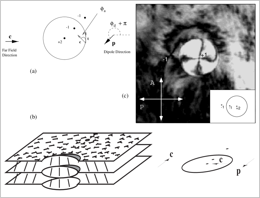
FIG. 1.:

FIG. 2.:

FIG. 3.:

FIG. 4.:

REFERENCES

- [1] Poulin, P., Stark, H., Weitz, D., and Lubensky, T.C., 1997, Science, 275, 1170.
- [2] Lubensky, T.C., Pettey, D., Currier, N., and Stark, H., 1998 Phys. Rev. E, 57, 1, 610.
- [3] Poulin P. and Weitz D., 1998 Phys. Rev. E, 57, 1, 626.
- [4] Meyer, R.B., 1972, Mol.Cryst. liq. Cryst., 16, 355.
- [5] Fang, J., Teer, E., Knobler, C.M., Loh, K., and Rudnick, J., 1997, Phys. Rev. E, 56, 2, 1859.
- [6] de Gennes, P., and Prost, J., 1993, The Physics of Liquid Crystals, 2nd Ed., Clarendon Press, Oxford.
- [7] Chandrasekhar, S., 1977, Liquid Crystals, Cambridge Univ. Press, Cambridge.
- [8] Chandrasekhar, S., and Ranganath, G.S., 1986, Adv. in Phys., 35, 6, 507.
- [9] Drzaic, P., 1995, Liquid Crystal Dispersions, World Scientific, New Jersey.
- [10] Hatwalne, Y., and Lubensky, T.C., 1995, Phys. Rev. E, 52, 6240.
- [11] Darren Link and Noel Clark (private communication).
- [12] Chaikin, P., and Lubensky, T.C., 1995, Principles of Condensed Matter Physics, Cambridge University Press, Cambridge.
- [13] Ranganath, G.S., 1976, Mol. Cryst. liq. Cryst. Lett., 34, 71.
- [14] Knobler, C.M., and Desai, R.C., 1992, Ann. Rev. Phys. and Chem., 43, 207.
- [15] Pindak, R., and Moncton, D., 1982, Phys. Today, 35, 5, 57.