Wetting and Capillary Condensation in Symmetric Polymer Blends:
A comparison between
Monte Carlo Simulations and Self-Consistent Field Calculations

Abstract

We present a quantitative comparison between extensive Monte Carlo simulations and self-consistent field calculations on the phase diagram and wetting behavior of a symmetric, binary (AB) polymer blend confined into a film. The flat walls attract one component via a short range interaction. The repulsion between monomers of different types leads to an upper critical solution point in the bulk. The critical point of the confined blend is shifted to lower temperatures and higher concentrations of the component with the lower surface free energy. The binodals close the the critical point are flattened compared to the bulk and exhibit a convex curvature at intermediate temperatures – a signature of the wetting transition in the semi-infinite system. We present detailed profiles of the two coexisting phases in the film and estimate the line tension between the laterally coexisting phases. Using the dependence of the thickness of the wetting layers and the shift of the chemical potential on the film width, we determine the effective interaction range between the wall and the $AB$ interface. Investigating the spectrum of capillary fluctuation of the interface bound to the wall, we find evidence for a position dependence of the interfacial tension. This goes along with a distortion of the interfacial profile from its bulk shape. Using an extended ensemble in which the monomer-wall interaction is a stochastic variable, we accurately measure the difference between the surface energies of the components, and determine the location of the wetting transition via the Young equation. The Flory-Huggins parameter at which the strong first order wetting transition occurs is independent of chain length and grows quadratically with the integrated wall-monomer interaction strength. We estimate the location of the prewetting line. The prewetting manifests itself in a triple point in the phase diagram of very thick films and causes spinodal dewetting of ultrathin layers slightly above the wetting transition. We investigate the early stage of dewetting via dynamic Monte Carlo simulations. We compare our findings to phenomenological descriptions and recent experiments.

1 Introduction

The behavior of confined complex fluids is of practical importance for various applications (e.g. adhesives, coatings, lubricants, zeolites). The confining surfaces give rise to packing effects and alter the conformations of macromolecules in its vicinity. In general one component (say A) may absorb preferentially at the surface, such that the wall is coated with a layer of the component with the lower surface free energy. The structural and thermodynamic properties of these wetting layers are of practical importance and of fundamental interest in the statistical mechanics of condensed matter. At phase coexistence of the binary mixture, the surface free energy in the semi-infinite system undergoes a transition, at which the thickness of the adsorbed $A$-rich layer diverges. This wetting transition may be continuous (second order wetting) or the thickness jumps from a finite value to infinity at the wetting transition temperature. The order of this transition and the temperature at which it occurs have attracted longstanding interest. [1, 2, 3, 4, 5, 6, 7] The walls are wetted by the $A$ component, if the difference $\Delta\sigma_{\rm w}$ between the surface free energy of the wall with respect to a B-rich bulk $\sigma_{WB}$ and the surface free energy against an A-rich bulk $\sigma_{WA}$ exceeds the free energy cost of an $AB$ interface $\sigma_{AB}$ at an infinite distance from the wall.[4, 8]

$$\Delta\sigma_{\rm w}=\sigma_{WB}-\sigma_{WA}>\sigma_{AB}\qquad\mbox{(Young equation)}$$ (1)

The spreading parameter $\Delta\sigma_{\rm w}-\sigma_{AB}$ controls the static and dynamic wetting behavior and is also accessible experimentally.[9] In structurally symmetric blends, the surface free energy difference $\Delta\sigma_{w}$ is dominated by the different enthalpic interactions of the monomers with the wall and thus $\Delta\sigma_{w}$ is largely independent of the molecular weight. In the strong segregation limit, the interfacial tension $\sigma_{AB}$ is also independent of chain length, and hence the wetting temperature is to leading order chain length independent. This is in marked contrast to the critical temperature of the mixture, which increases linearly with molecular weight. Thus, wetting in polymeric systems occurs far below the critical point,[10] unlike the generic situation in mixtures of small molecules.

If the mixture is confined into a pore or a thin film, this wetting transition is rounded. Also the unmixing temperature is reduced and the coexistence curve in the vicinity of the critical point is flattened compared to the bulk behavior. Moreover, the preferential interactions at the surfaces shift the coexistence pressure or chemical potential away from its bulk coexistence value.[11] At coexistence, the confined system phase separates laterally into A-rich domains which coexist with regions in which there are A-rich layers at the surfaces and the B-component prevails in the center of the film. The two phases are separated by interfaces, which run perpendicular to the surfaces. There is a delicate interplay between the wetting behavior of the semi-infinite system and the phase behavior in a thin film.[2, 11] In the temperature range between the critical temperature of the film and the wetting temperature, the thickness of the wetting layer at coexistence is determined by balancing the repulsion between the wall and the AB-interface, which favors a thick wetting layer, against the shift of the coexistence chemical potential, which suppresses the total amount of A component in the film.[12]

A binary polymer blend between walls is a suitable testing bed for these phenomenological ideas because the chain length $N$ constitutes an additional control parameter which can be varied without changing enthalpic interactions. Increasing the chain length $N$, we reduce bulk composition fluctuations, which are neglected in most phenomenological approaches, and there are powerful self-consistent field (SCF) techniques to describe the bulk and surface behavior. In addition, the larger length scales of the occurring phenomena due to the large size of the polymer coils facilitates applications of several experimental techniques. Consequently, the behavior of polymer blends in thin films has attracted abiding theoretical,[10, 13, 14, 15, 16] experimental[17, 18, 19, 20, 21] and simulational[22, 23, 24] interest. We briefly summarize some of the findings pertinent to the present paper below.

Nakanishi and Pincus[13] and Schmidt and Binder[10] have explored the wetting behavior at a wall of a binary polymer blend in the framework of a Cahn-Hilliard mean field theory. Employing a quadratic form of the surface free energy, they found first order wetting at low temperatures and second order transitions close to the critical point. Flebbe et al. [15] studied the confined system and revealed that pronounced differences between the wetting behavior of the infinite system and the capillary condensation in a film of thickness $D$ persist up to thicknesses which exceed the radius of gyration $R_{g}$ by roughly two orders of magnitude. However, both studies employed a square gradient (SG) approximation which is only adequate for describing composition variations on length scales larger than the coil extension – a situation which occurs close to the critical point. Moreover, estimating the parameters of the phenomenological surface free energy in the framework of a microscopic model is not straightforward. Self-consistent field techniques [20, 25, 26] overcome the limitations of the square gradient approximation and more microscopic treatments of the surface free energy contribution[27, 28, 29, 30, 31] have also been explored.

The detailed composition profiles at surfaces of polymer blends are experimentally accessible via a variety of techniques. Investigating structurally symmetric pairs of homopolymers via neutron reflectometry, Genzer et al. [20] have compared the experimental results to the square gradient theory [10] and self-consistent field calculations. They found qualitative agreement between experiments and theories. However, deviations from the quadratic dependence of the excess surface free energy on the surface composition are found. Similar deviations were reported by Scheffold et al.[17] and Budkowski et al.[18] using nuclear reaction analysis on random copolymers with different microstructures. In these experiments the wetting transition occurs presumably far below the critical point.

The reduction of the critical temperature and the crossover from 3D to 2D critical behavior have been studied in Monte Carlo (MC) simulations by Kumar and co-workers[23] and Rouault et al. [24, 32] These simulations have also been compared to mean field calculations.[27, 33] However, the simulations were restricted to symmetric blends and “neutral” walls (i.e., no preferential interaction between the walls and any component). In this limit, the coexistence chemical potential is not shifted away from its trivial bulk value $\Delta\mu_{\rm coex}=0$. Simulations of Wang and co-workers [22] extensively investigated the wetting behavior of a symmetric binary polymer blend at a hard wall which favors one component. Their simulation studies are closely related to the present investigation, but they did not systematically explore the effects of finite film thickness.

In this work, we explore the combined effect of confined geometry and preferential attraction of one component at the walls (“capillary condensation”) and investigate the interplay between the wetting behavior and the phase diagram in the confined geometry. We restrict ourselves to perfectly flat walls which both attract the same component via a short range potential. We obtain profiles across the film and of the interface between the laterally segregated phases. Employing finite size scaling and reweighting techniques we are able to measure the coexistence chemical potential as a function of the wall separation $D$ and investigate corrections to the Kelvin equation. We determine the phase diagram over a wide temperature range. Using a novel Monte Carlo scheme, we measure the surface free energy difference $\Delta\sigma_{w}$ and determine the wetting transition via the Young equation (1). We derive an approximate analytical expression of the wetting temperature in the strong segregation limit as a function of the interactions between the monomers and the wall and test this against our Monte Carlo simulation. At low temperatures the wetting transition is of first order and we estimate the location of the concomitant prewetting transition. We suggest an interpretation of recent experimental studies of spinodal dewetting of ultrathin polymer films[21] by Zhao and co-workers in terms of prewetting–like phase separation. This is illustrated via dynamic Monte Carlo simulations of ultrathin films. We measure the effective interaction range between the wall and the $AB$ interface and investigate the capillary fluctuation spectrum[34, 35] of the bound interface. We find evidence for a position dependence of the interfacial tension $\sigma$. We compare our results with phenomenological approaches and detailed self-consistent field calculations. The latter take due account of the chain conformations via a partial enumeration scheme[34, 36, 37] and incorporate details of the interactions at the surface. We find qualitative (and sometimes even quantitative) agreement between the simulations and the self-consistent field calculations without any adjustable parameter.

Our paper is arranged as follows: First, we give a phenomenological description of capillary condensation[12] and discuss its limitations. Then we introduce our coarse grained polymer model, give a brief synopsis of the simulation techniques, and detail the salient features of our self-consistent field scheme. In the main section we present a comparison between the results of our Monte Carlo simulations and self-consistent field calculations. We close with a brief discussion and an outlook on future work.

2 Background

We consider a binary polymer mixture confined into a thin film of lateral extension $L\times L$ and wall separation $D$. Let $\Phi$ denote the monomer volume fraction. Both types of structurally symmetric polymers consist of $N$ segments. The A-component of the blend is favored by both walls. The monomer-wall interactions are taken to be short ranged and the parallel walls are ideally flat. Phase coexistence comprises two laterally segregated phases. One of which is A-rich and exhibits only a minor compositional variation across the film. Following Parry and Evans,[12] we approximate its excess semi-grandcanonical potential $G$ per unit area with respect to the A-rich branch of the bulk coexistence curve by:

$$\frac{\Delta G_{A}}{L^{2}}=2\sigma_{WA}-\frac{\Phi}{N}D\left(\mu_{A}\langle\rho\rangle+\mu_{B}(1-\langle\rho\rangle)-\frac{\mu_{A}+\mu_{B}}{2}\right)=2\sigma_{WA}-\frac{\Phi}{2N}D\Delta\mu(2\langle\rho\rangle-1)$$ (2)

where $\sigma_{WA}$ denotes the surface free energy of the wall, $\mu_{A}$, $\mu_{B}$ the chemical potentials of A and B-polymers, $\Delta\mu=\mu_{A}-\mu_{B}$ their chemical potential difference, and $\langle\rho\rangle$ the composition of the A-rich phase at bulk coexistence. In the second phase the density of the B-component comes up to its bulk value at the center of the film, and this B-rich center region is separated from the wall by A-rich layers of width $l$. Provided that the layer thickness $l$ is larger than the microscopic length scale but much smaller than the wall separation $D$, the surface free energy of the wall $\sigma_{\rm WB}$ can be decomposed into the surface free energy $\sigma_{\rm WA}$, the free energy of an AB interface $\sigma_{AB}$, and the interaction $g(l)$ of this AB interface with the wall (complete wetting). Thus the excess potential takes the form:

$$\frac{\Delta G_{B}}{L^{2}}=\underbrace{2\sigma_{WA}+2\sigma_{AB}+2g(l)}_{2\sigma_{WB}}-\frac{\Phi}{N}2l\Delta\mu(2\langle\rho\rangle-1)+\frac{\Phi}{2N}D\Delta\mu(2\langle\rho\rangle-1)$$ (3)

Above the wetting temperature, the wall repels the AB interface and we take the short range interaction to be: $g(l)=A\exp(-\lambda l)$. Here $\lambda$ is a decay length which is of the same order as the correlation length of concentration fluctuations at bulk coexistence, as we shall discuss later. The thickness of the wetting layers $l$ is determined by the condition $\partial\Delta G_{B}/\partial l=0$, which yields:

$$l(D)=\frac{1}{\lambda}\ln\frac{NA\lambda}{-\Phi(2\langle\rho\rangle-1)\Delta\mu}$$ (4)

At phase coexistence the chemical potential difference is shifted such that the two phases have the same semi-grandcanonical potential:

$$\frac{1}{\Delta\mu_{\rm coex}}=-\frac{\Phi(2\langle\rho\rangle-1)}{2N\sigma_{AB}}\left(D-2l-\frac{2}{\lambda}\right)\qquad\mbox{(Kelvin equation)}$$ (5)

To leading order the shift of the chemical potential $\Delta\mu$ from the bulk coexistence value ($\Delta\mu=0$) is inversely proportional to the wall separation $D$ and the coefficient involves the $AB$ interfacial tension and the bulk composition. This expression rigorously describes the $D\to\infty$ limit.[6] Thus the inverse wall separation $1/D$ plays a similar role as the chemical potential (or the bulk composition) in complete wetting. The thickness $l$ of the wetting grows like $\ln D$, and the leading correction to the Kelvin equation $-\Delta\mu\sim 1/D$ are of relative order $\ln D/D$.[38]

Though this phenomenological description is expected to capture the qualitative behavior for very large wall separations and low temperatures, there are some limitations which might prevent a quantitative agreement with our Monte Carlo simulations. For very small wall separations $D<O(R_{g})$ ($R_{g}$: radius of gyration) of the film, neutron reflexion experiments reveal that the two $AB$ interfaces interact with each other;[19] the coupling of the two interfaces across the film has been neglected in the treatment above. More important, the detailed polymer conformations at the surface have been ignored. Polymers orient and deform at the hard walls.[24, 39] Since the length scale of these conformational changes is set by the radius of gyration $R_{g}$, one expects a distortion of the intrinsic interfacial profile and a concomitant modification of the effective interfacial tension for $l\sim\ln D<O(R_{g})$. Furthermore the repulsion of the interface by the wall involves many length scales (e.g. range of the wall-monomer interaction $d$, the width of the interface $w$, which controls the composition profile at the center of the interface, the bulk correlation length $\xi$, which sets the length scale in the wings of the interfacial profile.[40]) Thus a simple single exponential decaying interaction is only an effective description. However, these effects can be described duely in a self-consistent field framework.

Moreover, the mean field treatment neglects fluctuations. In the vicinity of the critical point, one expects a critical behavior belonging to the 2D Ising universality class.[32] Additionally, long wavelength fluctuations of the local position of the interface (“capillary waves”[41]) from its most probable value have been ignored. They can be described by a capillary fluctuation Hamiltonian:[42]

$$\frac{{\cal H}_{\rm eff}}{k_{B}T}=\int dx\;dy\;\left\{\frac{\sigma}{2}(\nabla\delta l(x,y))^{2}+\frac{1}{2}\frac{\partial^{2}g}{\partial l^{2}}\delta l^{2}\right\}$$ (6)

where $\sigma$ denotes the “effective” $AB$ interfacial tension in the thin film geometry, and $\delta l(x,y)$ measures the deviation of the local interfacial position from its average. Since we study a three dimensional system, which is at the upper critical dimension of wetting phenomena, capillary fluctuations do not alter the functional dependence of the layer thickness $l$ on the film size $D$.[4] However, the prefactor $1/\lambda$ in eq. (4) is multiplied by $(1+\omega/2)$,[43] where $\omega={k_{B}T}/({4\pi\xi^{2}\sigma_{AB}})$ is the wetting parameter. Thus, the range of the wall-interface interaction[44] is larger than in the self-consistent field theory, and the wetting layers are thicker, respectively. The Fourier components $a_{q}$ of the local interfacial position $\delta l$ are Gaussian distributed with width

$$\frac{2}{L^{2}\langle a_{q}^{2}\rangle}=\frac{\sigma}{k_{B}T}\left\{q^{2}+\frac{\partial^{2}g}{\sigma\partial l^{2}}\right\}=\frac{\sigma}{k_{B}T}\left\{q^{2}+\left(\frac{2\pi}{\xi_{\|}}\right)^{2}\right\}$$ (7)

Thus the spectrum[34, 35] yields information about the interfacial tension $\sigma$ and the parallel correlation length $\xi_{\|}$[4]

$$\xi_{||}=2\pi\sqrt{\sigma\left(\frac{\partial^{2}g}{\partial l^{2}}\right)^{-1}}=\sqrt{\frac{4\pi^{2}\sigma}{A\lambda^{2}}}\exp\left(\frac{\lambda l}{2}\right)\sim\sqrt{D}\sim\frac{1}{\sqrt{\Delta\mu}}\qquad\mbox{(complete wetting)}$$ (8)

$\xi_{\|}$ acts as a long wavelength cut-off for the capillary fluctuation spectrum.[4] Additionally, capillary fluctuations result in a broadening of the apparent interfacial width which increases like $\ln(\xi_{\|}).$[41] Since the parallel correlation length $\xi_{||}\sim\sqrt{D}$ growths with the wall separation $D$, we expect the squared interfacial width to depend logarithmically on the wall separation. This behavior contrasts the behavior of mixtures confined into a thin film with asymmetric walls. In this case a single interface occurs inside the thin film ($l\sim D$) and then a similar reasoning as above yields $\ln(\xi_{||})\sim D$.[41]

In the present study, we compare this phenomenological description to self-consistent field (SCF) calculations and Monte Carlo (MC) simulations quantitatively. This allows us to examine the effects discussed above and to obtain a detailed picture of the static structure and the thermodynamics of polymer blends in thin films.

3 Model and computational techniques

3.1 The bond fluctuation model and Monte Carlo (MC) technique

Investigating the universal behavior of confined polymer blends, we employ a coarse grained model that combines computational tractability with the important qualitative features of real polymeric materials: monomer excluded volume, monomer connectivity, and short range interactions. We employ the bond fluctuation model.[45] Much is known about the phase behavior[35, 46] and interfacial properties [22, 24, 32, 41, 34, 35, 47, 48] of this polymer model and the results have been compared to mean field calculations.[27, 34, 49] Within the framework of this model, each monomer blocks a whole unit cell of a 3D cubic lattice from further occupation. Monomers along a chain are connected by bond vectors of length $2,\sqrt{5},\sqrt{6},3$, and $\sqrt{10}$ lattice spacings. The blend comprises two structurally symmetric polymer species - A and B - of the same chain length $N=32$. This corresponds to roughly 150 repeat units in chemically realistic models. At a monomer density $8\Phi=0.5$ the model captures many features of a dense polymer melt. The size disparity between monomers and (single site) vacancies results in a fluid-like structure with pronounced packing effects on the monomer scale.[46] The structure of the monomer fluid is largely determined by the density and rather independent from the local composition or the temperature. Therefore we can lump the structure of the underlying bulk fluid into an effective coordination number z or a Flory-Huggins parameter $\chi$, which is accessible in the simulations via the intermolecular paircorrelation function. We would like to emphasize that our simulation techniques (e.g. extended ensemble technique to calculate the spreading parameter or the analysis of the capillary fluctuation spectrum[34, 35]) and our self-consistent scheme can be readily applied to off-lattice models.

Thermal monomer-monomer interactions are catered for by a short range square well potential extended over 54 neighboring lattice sites. This choice is motivated because it just includes all distances contributing to the first peak of the radial density correlation function. The contact of monomers of the same type lowers the energy by $\epsilon$, whereas contacts between unlike species increase the energy by $\epsilon$. Similar to previous work by Wang et al. [22], we consider a cuboidal system with a $L\times L\times D$ geometry. Periodic boundary conditions are applied in $x$ and $y$ direction and there are impenetrable, flat walls at $z=-1$ and $z=D$. Every $A$ monomer, which is in the d=2 layers adjacent to the walls reduces the energy by $\epsilon_{w}$, whereas each B-monomer in this wall interaction range increases the energy by the same amount. We keep $\epsilon_{w}/k_{B}T=0.16$ fixed during our simulations, thus the monomer-wall interaction is entropic in its character. This might be motivated by different packing behavior of the monomer species at the wall. In the following all lengths are measured in units of the lattice spacing.

The polymer conformations are updated via a combination of local random monomer hopping and slithering snake-like moves.[46] The latter ones relax the conformations roughly a factor $N$ faster than the local updates, and allow us to investigate longer chain lengths than in previous work.[22] We work in the semi-grandcanonical ensemble, i.e., at fixed temperature $k_{B}T/\epsilon$ and exchange potential $\Delta\mu/k_{B}T$, and the composition is allowed to fluctuate. These semi-grandcanonical moves consist for our symmetric blend of switching the chain type $A\rightleftharpoons B.$[46, 50]

The ratios between the semi-grandcanonical Monte Carlo moves and the ones which update the polymer conformations are adjusted to relax the composition of the blend and single chain properties on the same time scale. We employ: local hopping : slithering snake : semi-grandcanonical moves = 4:12:1

The coexistence curve in the confined geometry has been successfully determined in mixtures of simple fluids via the peak in the order parameter susceptibility or thermodynamic integration methods.[3] The former one is, however, restricted to the vicinity of the critical point, whereas the latter one involves the definition of a reference state in our polymer model.[51] In the present study, we employ the semi-grandcanonical moves in junction with a reweighting[52, 53] scheme to encourage the system to explore configurations in which both phases coexist in the simulation cell and the system “tunnels” often between the two coexisting phases. We obtain the reweighting factors via histogram analysis[54] of the joint composition-energy probability distribution of previous runs at higher temperatures; the procedure starts around the critical temperature $k_{B}T/\epsilon=69.3$. E.g. to obtain the preweighting factors at $k_{B}T/\epsilon=50$, we employ 5-9 simulations at intermediate temperatures. More technical details pertinent to the BFM can be found in Ref. [35]. This scheme permits an accurate location of the coexistence chemical potential and yields additional information about the free energy as a function of the composition of the system, the interfacial tension between coexisting phases[53], interactions between interfaces[35] and the wetting behavior.

3.2 Self-consistent field (SCF) calculations

We compare our Monte Carlo simulations to self-consistent field calculations[25, 36, 55, 56, 57, 58, 59, 60] which incorporate details of the polymer architecture[34, 36, 37, 59, 60] and surface interactions. The partition function of the binary polymer blend[55] containing $n_{A}$ A-polymers and $n_{B}$ B-polymers can be written in the form:

$${\cal Z}\sim\frac{1}{n_{A}!n_{B}!}\int\Pi_{\alpha=1}^{n_{A}}{\cal D}[r_{\alpha}]{\cal P}_{A}[r_{\alpha}]\Pi_{\beta=1}^{n_{B}}{\cal D}[r_{\beta}]{\cal P}_{B}[r_{\beta}]\exp\left(-\frac{\Phi}{k_{B}T}\int d^{3}r\;{\cal E}[\hat{\rho}_{A},\hat{\rho}_{B}]\right)$$ (9)

where the functional integrals ${\cal D}[r]$ sum over all polymer conformations and ${\cal P}[r]$ denotes the probability distribution characterizing the isolated (i.e. not mutually interacting) chain conformations in the confined geometry. ${\cal P}$ includes intramolecular interactions and the interaction with the wall, but not the pairwise interactions among different polymers. ${\cal E}$ represents a segmental free energy due to intermolecular interactions which is specified below. The dimensionless monomer density takes the form[55]:

$$\hat{\rho}_{A}(r)=\frac{1}{\Phi}\sum_{\alpha=1}^{n_{A}}\sum_{i_{A}=1}^{N_{A}}\delta(r-r_{\alpha,i_{A}})$$ (10)

The second sum runs over all monomers in the A-polymer $\alpha$, and a similar expression holds for $\hat{\rho}_{B}(r)$.

The probability distribution ${\cal P}[r]$ of an isolated single chain conformations between two hard walls is the product of the bare probability distribution ${\cal P}_{0}[r]$, which characterizes the noninteracting, single chain conformations in the bulk, and the Boltzmann weight ${\cal P}_{w}[r]$ of the interaction with the walls. The latter vanishes if one of the segments is located outside the interval $[0,D-2]$[61]. Otherwise it takes the form $\exp(\pm\epsilon_{w}n_{w}[r])$, where $n_{w}[r]$ is the number of segments in the wall interaction range $[0,d-1]$ and $[D-d-1,D-2]$. The $+$ or $-$ sign holds for A-polymers or $B$-polymers, respectively.

The segment free energy ${\cal E}$ comprises two contributions: a free volume term arising from hard core interactions and an energetic contribution from the repulsion of unlike species. Since the total density fluctuations in the melt are small, we approximate the free volume part by a simple quadratic expression introduced by Helfand[55], involving the knowledge of the inverse compressibility $\zeta$. This quantity has been measured in simulations of the athermal model; $\zeta=4.1$[62]. The repulsion between unlike monomer species is incorporated via a Flory-Huggins parameter $\chi=2{\tt z}\epsilon/k_{B}T$[46], where ${\tt z}$ denotes the number of monomers of other chains in the range of the square well potential of depth $\pm\epsilon$. In principle the number of intermolecular contacts can be evaluated for every chain conformation[63] as to include the coupling between chain conformations and energy. For simplicity we average the number of intermolecular interactions over all chain conformations and employ the effective coordination number which has been extracted from the intermolecular paircorrelation function $g(r)$ in the simulations of the bulk system. Moreover, neglecting the slight temperature dependence[64], we employ the value z=2.65 throughout our calculations. This value yields remarkably good agreement between SCF calculations and Monte Carlo simulations in our previous work on interfacial properties[34, 47, 49]. Hence, the segmental interaction free energy is taken to be[55]

$$\frac{{\cal E}[\rho_{A},\rho_{B}]}{k_{B}T}=\frac{\zeta}{2}\left(\rho_{A}+\rho_{B}-1\right)^{2}-\frac{1}{2}{\tt z}\epsilon(\rho_{A}-\rho_{B})\left(1+\frac{1}{2}l_{0}^{2}\partial^{2}_{\perp}\right)(\rho_{A}-\rho_{B})$$ (11)

$\partial_{\perp}$ denotes the spatial derivative perpendicular to the wall. The spatial range of the monomer-monomer interactions $l_{0}^{2}=\int dz\;g(r)z^{2}/\int dz\;g(r)\approx 16/9$, where the integration is extended over the range of the square well potential, has been estimated for the bond fluctuation model by Schmid[27]. This non-local energy density mimics the influence of the reduction of the number of pairwise intermolecular interactions due to the presence of the wall. The treatment of this “missing neighbor” effect is clearly an approximative one, and we expect it to be only of limited validity in the presence of the large concentration gradient at the wall.

Introducing auxiliary fields, we rewrite the many chain problem in terms of independent chains in external, fluctuating fields $W_{A}$ and $W_{B}$.

$${\cal Z}\sim\int{\cal D}[W_{A},W_{B},\Phi_{A},\Phi_{B}]\exp\left(-{\cal F}[W_{A},W_{B},\Phi_{A},\Phi_{B}]/k_{B}T\right)$$ (12)

where the free energy functional is defined by

$$f=\frac{{\cal F}[W_{A},W_{B},\Phi_{A},\Phi_{B}]}{\Phi k_{B}TV} = \frac{\bar{\rho}_{A}}{N_{A}}\ln\bar{\rho}_{A}+\frac{\bar{\rho}_{B}}{N_{B}}\ln\bar{\rho}_{B}+\frac{1}{V}\int d^{3}r\;{\cal E}(\Phi_{A},\Phi_{B})$$ (13)

$$-\frac{1}{V}\int d^{3}r\left\{W_{A}\Phi_{A}+W_{B}\Phi_{B}\right\}-\frac{\bar{\rho}_{A}}{N_{A}}\ln q_{A}[W_{A}]-\frac{\bar{\rho}_{B}}{N_{B}}\ln q_{B}[W_{B}]$$

$V$ is the volume of the system, $\bar{\rho}_{A}=\frac{n_{A}N_{A}}{\Phi V}=1-\bar{\rho}_{B}$ denotes the average A-monomer density, and $q_{A}[W_{A}]$ the single chain partition function of an $A$ polymer in the external field $W_{A}$. Using the definition of the monomer densities (cf. (10), we can write the latter as an explicit function of the location $r_{i}$ of the monomers along the $A$ polymer:

$$q_{A}[W_{A}]=\frac{1}{V}\int{\cal D}[r]{\cal P}_{A}[r]\exp\left(-\sum_{i=1}^{N_{A}}W_{A}(r_{i})\right)$$ (14)

The functional integral for the partition function cannot be solved, therefore we approximate it by the saddle point of the integrand. The values of the collective variables, which extremize eq. (13) are denoted by lower case letters. They are determined by the equations:

$$\frac{\delta{\cal F}}{\delta\rho_{A}}=0 \Rightarrow w_{A}=\frac{\delta}{\delta\rho_{A}}\int d^{3}r\;{\cal E}(\rho_{A},\rho_{B})=\zeta(\rho_{A}+\rho_{B}-1)-{\tt z}\epsilon\left(1+\frac{1}{2}l_{0}^{2}\partial_{\perp}^{2}\right)(\rho_{A}-\rho_{B})$$ (15)

$$\frac{\delta{\cal F}}{\delta w_{A}}=0 \Rightarrow \rho_{A}=\frac{\bar{\rho}_{A}V}{N_{A}q_{A}}\frac{\delta q_{A}}{\delta w_{A}}$$ (16)

and similar expressions for $w_{B}$ and $\rho_{B}$. The saddle point integration approximates the original problem of mutually interacting chains by one of a single chain in an external field, which is determined, in turn, by the monomer density. The coupling between composition and polymer conformations is retained; however, composition fluctuations and the coupling between the individual polymer conformations and the effective coordination number z are ignored. In inhomogeneous situations this coupling gives rise to a position-dependence of z [47].

To determine the phase diagram we calculate the chemical potential difference $\Delta\mu$ and the semi-grandcanonical potential $G$ according:

$$\frac{\Delta\mu}{k_{B}T}=\frac{\partial{\cal F}}{k_{B}T\partial n_{A}}=N\frac{\partial f}{\partial\bar{\rho}_{A}}$$ (17)

$$\frac{G(\Delta\mu)}{kT\Phi V}=f-\frac{\Delta\mu}{k_{B}T}\frac{\bar{\rho}_{A}(\Delta\mu)}{N}\qquad\mbox{+linear terms in $\Delta\mu$}$$ (18)

Note that we have specialized here to the case $N_{A}=N_{B}=N$ while eq. (9)-(16) still hold for the general situation of chain length asymmetry. At coexistence, the phases have equal semi-grandcanonical potential $G(\Delta\mu)$.

We evaluate the single chain partition function via a partial enumeration scheme[36, 37, 34, 59, 60]. Using MC simulations of the pure melt, we generated 81,920 independent polymer conformations at temperature $\epsilon=0.02k_{B}T$ according to the distribution ${\cal P}_{0}$. Since the chain conformations are almost temperature independent, we use the same sample to extend the SCF calculations to different temperatures. Rotating and translating those original conformations, we obtain between 3932160 and 15726640 polymer conformations. (Note that only the perpendicular coordinates of the chains are employed.) The position of the first monomer is chosen randomly with a uniform distribution inside the interval $[0,D-2]$ along the $z$-axis. The polymer conformation is discarded (${\cal P}_{w}=0$) if any segment is located outside this interval. Otherwise, the number of segments within the two nearest layers to the walls is properly counted and the Boltzmann factor of the interaction with the wall yields the weight ${\cal P}_{w}$. Note that the procedure incorporates the coupling between chain extensions parallel and perpendicular to the walls; an effect which is ignored in the Gaussian chain model. Moreover, it incorporates the chain architecture on all length scales without any adjustable parameter[34]. Within this framework, the A-monomer density (c.f. eq. 16) is the statistical average of independent A-polymers with distribution ${\cal P}_{w}$ in the external field $w_{A}$:

$$\rho_{A}(r)=\bar{\rho}_{A}\frac{\sum_{\alpha=1}^{C}{\cal P}_{w}[r]\frac{1}{N_{A}}\sum_{i=1}^{N_{A}}V\delta(r-r_{\alpha,i})\exp\left(-\sum_{i=1}^{N_{A}}w_{A}(r_{\alpha,i})\right)}{\sum_{\alpha=1}^{C}{\cal P}_{w}[r]\exp\left(-\sum_{i=1}^{N_{A}}w_{A}(r_{\alpha,i})\right)}$$ (19)

Other single chain quantities (e.g. orientations, chain end densities) are given by corresponding averages over independent chains in the fields $w_{A}$ and $w_{B}$.

We expand the spatial dependence of the densities and fields in a Fourier series[65] $\{f_{1}(z)=1$ and $f_{k}(z)=\sqrt{2}\cos(2\pi k(z+1)/D)$ for $k=2,(D+1)/2\}$; e.g., $w_{A}(r)=\sum_{k=1}^{(D+1)/2}w_{A,k}f_{k}(z)$. This allows only for solutions which are symmetric around the middle of the film. We assume the breaking the symmetry in the $z$ direction to be thermodynamically less favorable than lateral phase separation[15]. Certainly, other decomposition schemes can be chosen[66] which allow for asymmetric profiles. However this requires a larger number of basis functions and, hence, increases the computational effort. Defining the contribution of an $A$ polymer conformation $\alpha$ to the Fourier component $k$ according to $\phi_{k}(\alpha)=\sum_{i=1}^{N_{A}}f_{k}(r_{\alpha,i})$ we rewrite the above equation in the form:

$$\rho_{A,k}=\bar{\rho}_{A}\frac{\sum_{\alpha=1}^{C}{\cal P}_{w}[r]\phi_{k}(\alpha)/N_{A}\exp\left(-\sum_{k=1}^{(D+1)/2}w_{A,k}\phi_{k}(\alpha)\right)}{\sum_{\alpha=1}^{C}{\cal P}_{w}[r]\exp\left(-\sum_{k=1}^{(D+1)/2}w_{A,k}\phi_{k}(\alpha)\right)}$$ (20)

For a fast evaluation of the above average we keep all $\phi_{k}(\alpha)$ ($k=1,\cdots,(D+1)/2$ and $\alpha=1,\cdots,C$) in the computer memory. This poses rather high memory demands (several Gbytes) and we employ a massively parallel CRAY T3E computer, assigning a subset of conformations to each processing element. We use up to 512 processors in parallel. The resulting set of $D-1$ non-linear equations is solved via a Newton-Raphson like method. Usually we achieve convergence within 4-7 iterations.

4 Results

4.1 Phase coexistence in a thin film

We begin by exploring the qualitative features of phase coexistence and illustrating our simulation methodology. The averaged 2D composition profiles of the laterally segregated, coexisting phases in a thin film of geometry $L_{x}\times L_{y}\times D$ with $L_{x}=164$ and $L_{y}=D=48$ are presented in Figure 1. The simulations are performed at constant composition, i.e. no semi-grandcanonical identity switches are employed. The grey scale indicates the composition; A-rich regions are lighter shaded than B-rich ones. The two interfaces are parallel to the $yz$ plane and are free to move in $x$-direction. Only their distance is fixed by the overall composition. Thus we average the profiles with respect to the instantaneous center of gravity of $B$ polymers in each configuration. The 2D profiles resemble qualitatively the results of 2D SCF calculations of Schlangen et al.[67]; however, our profiles are broadened by capillary waves[41]. The profiles at the two temperatures are qualitatively different. At the higher temperature (a) $\epsilon/k_{B}T=0.02$ the interface between the $A$-rich and $B$-rich phases is quite broad and even in the $B$-rich phase, there is an $A$-rich layer at the wall. This corresponds to the situation above the wetting transition. At the lower temperature (b) $\epsilon/k_{B}T=0.08$, the profile is much sharper and there is no $A$-rich layer at the wall in the $B$-rich phase. Moreover, the interface between the coexisting phases meets the wall at a finite angle. Thus the $A$ polymers do not wet the wall. Unfortunately, the film width $D=48$ is not large enough to extract the contact angle $\Theta_{e}$ of a macroscopic droplet reliably, because the interface exhibits a pronounced curvature. Thus it is difficult to quantify a contact angle, and systems with opposing boundary fields might yield more reliable estimates. Using the independent determined interfacial tension $\sigma_{AB}=0.0436k_{B}T$ and the difference in the surface free energy $\Delta\sigma_{w}=0.0397k_{B}T$ (see below), we estimate the contact angle $\Theta_{e}$ for a thick film to: $\cos\Theta_{e}=\Delta\sigma_{\rm w}/\sigma_{AB}\approx 0.91=\cos 25^{o}$

Employing semi-grandcanonical identity changes in addition, we allow the overall composition of the system to fluctuate. The reweighting technique[52, 53] permits us to explore a wide range of compositions $\rho$ and the probability distribution $P(\rho)$ yields information about the free energy $F(\rho)=-k_{B}T\ln P(\rho)+\mbox{const}$. The distributions in a thin film (in the same geometry and temperature as in Figure 1 (a)) and in the bulk are displayed in Figure 2 (a). The chemical potential difference $\Delta\mu$ has been adjusted to its coexistence value (cf. next section). The locations of the two peaks correspond to the composition of the coexisting phases. The distribution of the bulk system is symmetric around $\rho=0.5$. In the thin film, however, the composition of the B-rich peak is shifted to higher values of $\rho$ due to the wetting layers at the walls. Moreover, the $A$-poor peak is broader than the $A$-rich one. The plateau in the probability distribution indicates that the two interfaces can change their distance (and thereby alter the composition) at negligible free energy costs. Hence the interfaces do not interact, and we calculate the interfacial tension[68] according to $\sigma/k_{B}T=-\ln\left(P_{\rm max}/P_{\rm min}\right)/2L_{y}D$. In the confined blends, $\sigma D$ rather corresponds to the line tension $\Gamma$ between the coexisting phases in the film. The MC data in Figure 2 (a) yield $\sigma=0.0054(1)k_{B}T$ for the bulk interfacial tension and $\Gamma=0.051(5)k_{B}T$ for the line tension in the film of width $D$. In a crude approximation, the line tension $\Gamma$ is proportional to the bulk interfacial tension $\sigma$, and the effective length of the $AB$ interface $D-2l$ across the film, where $l$ denotes the thickness of the $A$-rich wetting layer in the $B$-rich phase. Of course, this is an upper bound to the free energy cost of the $AB$ interface in a film, because the system chooses rather a curved interface (cf. Figure 1 (a)) and even in the middle of the film there is no region where the interface is appropriately described by the bulk behavior. Moreover, $\Gamma$ vanishes at the critical temperature of the thin film, whereas the bulk interfacial tension becomes zero at the higher bulk critical temperature. Upon decreasing the temperature the interfacial tension $\sigma$ and the line tension $\Gamma$ increase. Figure 2 (b) presents the temperature dependence of $\Gamma$ and the ratio $\Gamma/\sigma(D-2l)$. We estimate the thickness $l$ via $l=\frac{\rho-(1-\langle\rho\rangle)}{2\langle\rho\rangle-1}\frac{D}{2}$, where $\rho$ denotes the composition of the $B$-rich phase and $\langle\rho\rangle$ the composition in the bulk. The ratio $\Gamma/\sigma(D-2l)$ is smaller than one and grows upon decreasing the temperature.

4.2 The phase behavior of the bulk and the confined system

To determine the phase behavior of the confined system in the semi-grandcanonical ensemble, we locate the coexistence curve in the two-dimensional parameter space of temperature $k_{B}T/\epsilon$ and chemical potential difference $\Delta\mu/k_{B}T$, employing various concepts of finite size scaling theory. At coexistence, the two phases have the same semi-grandcanonical potential $G$ and we employ the equal weight criterion[69] for the probability distribution $P(\rho,\epsilon,\Delta\mu)$ of the density at fixed temperature and chemical potential; i.e., we adjust the chemical potential such that[46]:

$$\int_{0}^{\rho^{*}}P(\rho,\epsilon,\Delta\mu)d\rho=\int_{\rho^{*}}^{1}P(\rho,\epsilon,\Delta\mu)d\rho\qquad\mbox{with}\qquad\rho^{*}=\int_{0}^{1}\rho P(\rho,\epsilon,\Delta\mu)d\rho$$ (21)

This definition is very accurate for locating the coexistence curve below the critical temperature even for systems with moderate linear dimensions $L$. However it entails corrections of the order $L^{-(1-\alpha)/\nu}\sim 1/L$[48] in the value of the critical composition due to field mixing effects, where we have used 2D Ising values for the critical exponents $\alpha$ of the specific heat and $\nu$ of the correlation length. Remember that the “field mixing” arises from a coupling between order parameter and energy density, whose singular part involves the critical exponent $1-\alpha$[71]. Below the critical point, we use the system size $96\times 96\times 48$ (for $\epsilon/k_{B}T\leq 0.03$) or $48\times 48\times 48$ (for $\epsilon/k_{B}T>0.03$) and $\epsilon_{w}/k_{B}T=0.16$. To locate the critical point we use substantially larger lateral extensions $L\leq 264$.

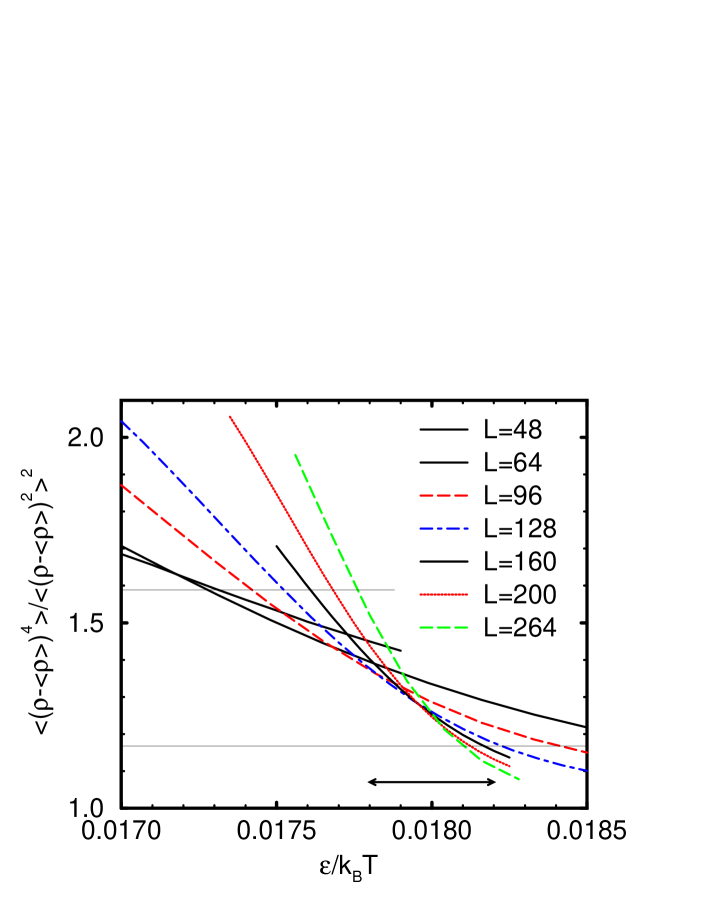
Figure 3: Fourth order cumulant intersection along the coexistence curve to determine the critical temperature for $D=48$ and $\epsilon_{\rm w}=0.16$. The error marks the uncertainty in the critical temperature $\epsilon_{c}=0.0180(2)$. The horizontal lines mark the values of the cumulant of the 3D Ising (upper) and 2D Ising (lower) model.

Along the coexistence curve and its continuation that persists in finite-size systems, we employ the cumulants of the composition probability distribution[70] to locate the critical point. Finite size scaling theory implies that the moments of the order parameter $\langle(\rho-\langle\rho\rangle)^{l}\rangle$ scale at criticality like $L^{-l\beta/\nu}$, where $\beta$ and $\nu$ are the critical exponents of the order parameter and the correlation length, respectively. Therefore, the ratio $\langle(\rho-\langle\rho\rangle)^{4}\rangle/\langle(\rho-\langle\rho\rangle)^{2}\rangle^{2}$ becomes independent of the system size $L$ at criticality. Plotting this cumulant ratio vs. inverse temperature for different linear dimensions, one hence expects in the ideal case all curves to intersect in a common point, which yields the critical temperature. Since this method involves only even moments of the order parameter, it is rather insensitive to “field mixing” corrections[71]. Figure 3 displays the fourth order cumulant ratio of our simulations for wall separation $D=48$. The cumulants for small lateral extension $L$ do not intersect at a common temperature, because the data fall into the crossover regime between three dimensional and two dimensional critical Ising-like behavior. The values of the cumulant for 3D and 2D Ising criticality[72] are also shown in the figure. Only, for aspect ratios $L/D>3$ a common intersection point gradually emerges around $\epsilon_{c}/k_{B}T=0.0180(2)$, which is our estimate for the critical temperature in the film. The corresponding value of the critical composition is $\rho_{Ac}=0.686(4)$. Using the data for the three largest lateral extensions $L=160,200,264$ and assuming 2D Ising critical behavior ($\beta=1/8$), we obtain $\rho_{\pm}=\rho_{c}\pm 0.46(2)\left({(\epsilon-\epsilon_{c})}/{k_{B}T}\right)^{\beta}$ for the binodal in the vicinity of the critical point. For a full understanding of the data in Figure 3 combined analysis of crossover scaling and finite size scaling would be required, which is still a formidable problem for the theory of critical phenomena in general.

The phase diagram of the bulk system and a film of width $D=48$ is presented in Figure 4 (a). The phase diagram of the bulk system is symmetric around $\rho=0.5$ and exhibits 3D Ising-like critical behavior (i.e. $\beta=0.325$). The binodal of the confined system near the critical point are flatter than in the bulk, indicating 2D Ising critical behavior[24]. The critical temperature in the film ($D=48$ and $\epsilon_{w}/k_{B}T=0.16$) is reduced by $20\%$ compared to the bulk. Note that this effect is much more pronounced than in the absence of preferential absorption of the A-component at the surfaces. Simulations of the symmetric system $D=48$ without preferential interactions $\epsilon_{w}=0$[24] found a suppression of the critical temperature by only $4\%$.

There are two pronounced changes of curvature in the A-poor branch of the binodal $\rho_{-}(T)$. The convex curvature around $k_{B}T/\epsilon\approx 20$ is the fingerprint of the wetting transition of the semi-infinite system. Around the wetting temperature, the wall-interface interaction $g(l)$ changes from attractive (for $T<T_{\rm wet}$) to repulsive. Assuming that $A(T)$ grows upon increasing $T$ for $T>T_{\rm wet}$ and $\lambda\sim 1/\xi\sim 1/R_{g}$ is only weakly temperature dependent we can combine eqs. (4) and (5) to obtain for large $D$:

$$\rho_{-}\approx\frac{2l}{D}\approx\frac{2}{\lambda D}\ln\left(\frac{A(T)\lambda D}{2\sigma_{AB}}\right)$$ (22)

which describes the convex portion qualitatively. For temperatures far below the wetting temperature, the composition is given by: $\rho_{-}\sim\exp(-\chi N)$, while we find critical behavior around $T_{c}$. In both temperature regimes the binodal is concave. A similar shape of binodals is also observed in confined Lennard-Jones mixtures[73].

Figure 4 (c) presents the results of our SCF calculations. Qualitatively similar to the MC results, the critical point of the film is shifted to a lower temperature and a higher concentration of the A-component. SCF calculations and MC simulation agree nicely on the critical concentration. The reduction of the critical temperature by $10\%$ is however somewhat smaller than in the MC simulations. Of course, both the bulk and the thin film critical point exhibit mean field critical behavior with $\beta=1/2$, and the critical temperatures of the bulk and the film are overestimated by the SCF theory. This overestimation is larger in 2D ($T_{c}^{\rm MF}/T_{c}^{\rm MC}=1.38$) than in the bulk ($T_{c}^{\rm MF}/T_{c}^{\rm MC}=1.22$). At intermediate temperatures we also find a convex shape of the binodal in our SCF calculations.

The coexistence chemical potential is presented in Figure 4 (b) and (d) for the MC simulations and for the SCF calculations, respectively. The chemical potential is shifted away from its coexistence value. For temperatures above the wetting transition, eq. (5) can be simplified to

$$\frac{\Delta\mu_{\rm coex}D}{k_{B}TN}=-2b\sqrt{\chi/6}\qquad\mbox{(wet wall)}$$ (23)

This estimate is also displayed in the figures. It describes the qualitative behavior above $k_{B}T/\epsilon\approx 20$. At lower temperatures, the coexistence value of the chemical potential difference becomes temperature independent. As we shall explain below, this is again a signature of vicinity to the wetting transition in the semi-infinite system.

4.3 The wetting transition of the semi-infinite system

At the B-rich branch of the bulk coexistence curve ($\Delta\mu/k_{B}T\to 0^{-}$), there is a wetting transition at which the thickness $l$ of the A-rich layer at the wall of a semi-infinite system diverges [1, 2, 4]. Since our monomer-wall interactions $\epsilon_{w}/k_{B}T=0.16$ are rather strong compared to the monomer-monomer interactions at the critical temperature $\epsilon/k_{B}T_{c}=0.0180(2)$, we expect the wetting transition to occur far below the critical point. As we shall see, the transition is first order at low temperatures, i.e. the thickness $l$ of the absorbed layer jumps discontinuously from a finite value to infinity upon approaching the wetting temperature $k_{B}T_{\rm wet}/\epsilon$ from below.

Wetting occurs according to the Young equation (1) when the surface free energy difference $\Delta\sigma_{w}$ exceeds the bulk interfacial tension. By virtue of the symmetry of our polymer model with respect to exchanging the labels $A$ vs. $B$, the surface free energy $\sigma_{WA}$ of a wall with interaction strength $\epsilon_{w}$ with respect to an A-rich bulk equals the free energy cost of a wall with interaction strength $-\epsilon_{w}$ (i.e. favoring B-monomers) with respect to a B-rich bulk. Thus the free energy difference can be obtained directly via thermodynamic integration at $\Delta\mu=0^{-}$:

$$\Delta\sigma_{\rm w}=\frac{1}{2L^{2}}\Big{\{}G(\epsilon_{w})-G(-\epsilon_{w})\Big{\}}=\frac{1}{2L^{2}}\int_{-\epsilon_{w}}^{\epsilon_{w}}de_{\rm w}\;\;\frac{\partial G}{\partial e_{\rm w}}=-d\Phi\int_{-\epsilon_{w}}^{\epsilon_{w}}de_{\rm w}\;\;\langle\phi_{\rm wall}(e_{\rm w})\rangle\qquad\mbox{(B-rich bulk)}$$ (24)

(for our choice of the Hamiltonian) where the surface composition $\phi_{\rm wall}$ denotes the difference of the number of A-monomers and B-monomers in the $d=2$ nearest layers at the wall normalized by $2d\Phi L^{2}$. If the mixture was completely incompressible (i.e. in the absence of packing effects at the wall), the surface composition would range between $-1$ and $1$.

For a B-rich bulk and temperatures below the wetting transition, the surface composition $\phi_{\rm wall}$ is rather independent of the monomer-wall interaction $\epsilon_{w}$ and close to -1. If the wetting transition is a strong first order transition, the thickness of the absorbed layer will remain small, as will the deviation of $\phi_{\rm wall}$ from -1. Thus eq. (24) yields the estimate $\Delta\sigma_{\rm w}\approx 2d\Phi\epsilon_{w}$. $\Delta\sigma_{\rm w}$ is dominated by the monomer-wall interaction; the entropy loss of the polymers at the wall is assumed to be the same for both species and hence does not affect $\Delta\sigma_{\rm w}$ in our model. Using the expression $\sigma_{AB}/k_{B}T=b\Phi\sqrt{\chi/6}$ ($b=3.05$ [47]: statistical segment length) for the interfacial tension in the strong segregation limit (SSL)[2], we get the following estimate for first order wetting transition temperature in the strong segregation limit:

$$\chi_{\rm wet}\approx 24\left(\frac{\epsilon_{w}d}{b^{2}k_{B}T}\right)^{2}\qquad\mbox{(SSL)}$$ (25)

which depends quadratically on the wall-monomer interaction strength $\epsilon_{w}d$ and is independent of the chain length $N$. Using the parameters of our simulations, the above equation yields $\epsilon/k_{B}T_{\rm wet}\approx 0.05$. If the monomer-wall interaction $V_{WA(B)}(z)$ were not of square well type, we would replace $\epsilon_{w}d$ by the integrated interaction strength.

$$\epsilon_{w}d=\int dz\;\Big{[}V_{WB}(z)\rho_{B}(z)-V_{WA}(z)\rho_{A}(z)\Big{]}$$ (26)

Using $\langle\rho\rangle=\exp(-\chi N)$ in the strong segregation limit (SSL) we can rewrite the expression above in terms of the bulk composition:

$$\frac{\epsilon_{w}}{k_{B}T}=\sqrt{\frac{b^{2}}{24Nd^{2}}\ln\frac{1}{\langle\rho\rangle}}\qquad\mbox{(SSL)}$$ (27)

However, for any finite film width $D$ the B-rich phase is not stable for $-\Delta\mu_{\rm coex}({\rm bulk})=0^{-}<-\Delta\mu<-\Delta\mu_{\rm coex}(D)$, and the thermodynamically stable phase at the bulk coexistence chemical potential is A-rich. Thus there is no wetting transition in a thin film in thermal equilibrium. We estimate the coexistence value of the chemical potential difference below the wetting transition in the bulk to be:

$$-\frac{\Phi D\Delta\mu_{\rm coex}}{2N}=\Delta\sigma_{w}=2d\Phi\epsilon_{w}\qquad\Rightarrow\qquad\frac{\Delta\mu_{\rm coex}D}{k_{B}TN}=-4\frac{d\epsilon_{w}}{k_{B}T}\qquad\mbox{(dry wall)}$$ (28)

by replacing $\sigma_{AB}$ by $\Delta\sigma_{w}$ in eq. (5). Above the wetting transition in the bulk, the chemical potential difference depends on the strength of the monomer-monomer interaction $\epsilon$ (or $\chi$), whereas below the wetting temperature it is independent of $\chi$ but depends on the monomer-wall interaction $\epsilon_{w}$. Therefore we attribute the change in the $\Delta\mu-T$ phase diagram (Figure 4 (b,d)) around $k_{B}T/\epsilon\approx 14$ to the wetting transition in the semi-infinite system. If we had chosen an enthalpic surface interaction, the chemical potential would depend linearly on the temperature below the wetting temperature, instead of being temperature independent.

To investigate the influence of the wetting transition in the bulk on the behavior of the confined system further, we calculate the composition dependence of the free energy close to the first order wetting transition in the SCF scheme. At low concentration of the A-component, the A-rich wetting layers are bound to the wall (“dry” state) and the free energy of this state with respect to the thermodynamically stable A-rich phase at $\rho\approx 1$ is $2\Delta\sigma_{\rm wall}L^{2}$. Upon increasing the composition the thickness of the A-rich layers increases and for large layer thickness ($\lambda D\gg\lambda l\gg 1$) the excess free energy is given by the interfacial tension $2\sigma_{AB}L^{2}$ (“wet” state). A plateau in the free energy indicates that the two interfaces are only weakly interacting. Both states are separated by a free energy barrier of height $2\gamma L^{2}>0$; thus the wetting transition is first order. For even higher concentrations the two $AB$ interfaces attract each other and finally annihilate to form the stable $A$-rich phase. The results of the SCF calculations for $\epsilon/k_{B}T=0.0575$ and $D=49,81$ and $137$ are presented in Figure 5 (a). One clearly identifies the “dry state” and the plateau, which corresponds to the “wet” state. Both are separated by a free energy barrier $\gamma/k_{B}T\approx 0.0027(8)$. Note that the data depend on the wall separation $D$ even for film widths as large as $D=137\approx 20R_{g}$. The surface free energy difference $\Delta\sigma_{w}$ and the interfacial tension decrease both upon increasing the film width. However, the effect is slightly more pronounced for the interfacial tension, thus using the data for thin films, we would systematically overestimate the wetting temperature. Increasing the film width $D$ still further in our SCF calculations, exceeds our computational facilities. The calculation of a single profile ($D=137$ and $7,863,320$ polymer conformations) requires about 10 minutes on 512 T3E processors and about 8 Gbyte of memory. Thus we use the width $D=137$ to explore the wetting behavior in the SCF calculations.

Though the wetting temperature can be estimated in the MC simulation via the scheme above (cf. Appendix), it is limited to rather small system sizes, because the configurations relax via a slow diffusion of the $AB$ interfaces across the film. Moreover, the connection between the composition of the system and the thickness of the wetting layers is more involved. The probability distribution of the composition for $\epsilon/k_{B}T=0.0695$ is presented in Figure 5 (b) for system geometry $48\times 48\times 48$. It shows qualitatively the same behavior as the free energy in the SCF calculations. The equal probability of the “dry” state and the free interfaces gives an estimate for the wetting temperature $\epsilon_{\rm wet}/k_{B}T\approx 0.0695$. Upon increasing the temperature, the “dry” state becomes metastable and ceases to exist even as a metastable state around $\epsilon/k_{B}T=0.063$ (cf. Figure 5 (b inset)). Thus the spinodal temperature is about $10\%$ higher than the wetting temperature. In view of the dependence of our SCF results on the wall separation $D$, we expect that our simulation data for $D=48$ are affected in a similar manner. Indeed, the plateau value is slightly higher than the interfacial tension $\sigma$ (displayed as a dashed horizontal line) obtained from the simulations of a system with periodic boundary conditions and $36\times 36\times 64$ geometry. Thus the wetting temperature is slightly lower than the estimate above.

In view of these difficulties, it is interesting to compare different methods for locating the wetting transition. Within the mean field framework, the wetting layers in a film are metastable for $\gamma>0$, and their lifetime $\tau$ in the MC simulations increases with the lateral extension $L$ like $\tau\sim\exp(\gamma L^{2})$. Upon increasing the temperature $k_{B}T/\epsilon$ the coefficient $\gamma$ decreases and vanishes at the wetting spinodal. Of course, fluctuations cause a pronounced rounding of the spinodal when $\gamma L^{2}\sim O(k_{B}T)$. The observation of this metastability has been used previously to determine the location of the wetting transition and its order by Wang et al. [22]. To determine the spinodal point we measure the surface order parameter $\phi_{\rm wall}$ as a function of the temperature $k_{B}T/\epsilon$. We use rather large lateral extensions $L$ to increase the lifetime of the metastable state and large film widths $D$ to avoid interactions between the two $AB$ interfaces. Using the SCF estimate, we obtain $\gamma L^{2}\approx 25k_{B}T$ for $L=96$ at the wetting transition. The simulation data for the system geometry $96\times 96\times 80$ and $128\times 128\times 128$ are presented as open symbols and filled symbols in Figure 5(c), respectively. In the thermodynamically stable A-rich phase there are exclusively A-monomers near the wall and the surface composition is almost temperature independent. In the metastable B-rich phase, the surface composition at low temperatures is B-rich and the surface order parameter increases rapidly for $\epsilon/k_{B}T<0.7$. This increase goes along with a pronounced increase of the surface composition fluctuations in the metastable phase, as shown in the inset. We identify this change of the surface order parameter $\phi_{\rm wall}$ and the observation that no metastable B-rich phase could be detected in our simulations for $\epsilon/k_{B}T<0.065$ as the signature of the spinodal and use $\epsilon/k_{B}T_{sp}=0.065(3)$ as our estimate for the spinodal temperature.

If the $AB$ interfacial tension has been measured independently (e.g. via reweighting techniques[47, 53, 68] or the spectrum of capillary fluctuations[34, 35]), we can use the Young equation (1) and eq. (24) to determine the wetting temperature. However, rather than measuring the surface order parameter $\phi_{\rm wall}$ for many values of the wall interaction strength $e_{\rm w}$, we use an expanded ensemble[52] in which the wall-monomer interaction strength $e_{\rm w}$ is a stochastic degree of freedom which assumes values between $-\epsilon_{w}$ and $+\epsilon_{w}$. This permits us to calculate the free energy difference in a single simulation run:

$${\cal Z}\sim\sum_{-\epsilon_{w}\leq e_{\rm w}\leq\epsilon_{w}}Z(e_{\rm w})/W(e_{\rm w})=\sum_{e_{\rm w}}W^{-1}(e_{\rm w})\exp(-G(e_{\rm w})/k_{B}T)$$ (29)

where $Z(e_{\rm w})$ is the semi-grandcanonical partition function at fixed temperature, exchange potential and wall interaction. We chose the preweighting factors $W(e_{\rm w})\sim\exp(-G(e_{\rm w})/k_{B}T)$ as to achieve uniform sampling of all $e_{\rm w}$ states. A good initial estimate of the preweighting factors is given by $W(e_{\rm w})=\exp(-2d\Phi L^{2}e_{\rm w}/k_{B}T)$.

Figure 5 (d) displays the surface composition $\langle\phi_{\rm wall}\rangle$ at $\epsilon/k_{B}T=0.07$,$\Delta\mu=0^{-}$ and $-0.16\leq\epsilon_{w}/k_{B}T\leq 0.16$. The bars in the figure do not denote statistical errors but the variance of the distribution of the surface composition. Thus the distributions of $\phi_{\rm wall}$ at the different values of the monomer-wall interaction overlap strongly. The increase of the monomer-wall interaction $\epsilon_{w}$ shifts the surface composition to higher values and its fluctuations increase. The crude estimate $\langle\phi_{\rm wall}\rangle=-1$ is also shown in the figure. Values of $|\phi_{\rm wall}|>1$ can be attributed to compressibility effects: Assuming that the system contains only B-chains, we can decrease the wall interaction energy by changing the monomer density in the first $d$ layers at the wall. This deviation from the bulk density costs entropy and we approximate it by a quadratic compressibility term (cf. eq. (11)). Balancing these two terms we obtain $\langle\phi_{\rm wall}\rangle=-(1-\epsilon_{w}/\zeta)$. The linear dependence of $\phi_{\rm wall}$ describes the simulational data qualitatively when the walls favor the majority phase in the bulk (i.e. $\epsilon_{w}<0$), though the effect is somewhat more pronounced than the estimate above with the bulk value $\zeta=4.1$ of the compressibility at infinite temperature.

In the simulations we divide the interval [$-\epsilon_{w},+\epsilon_{w}$] into 16 subintervals, and the MC scheme incorporates moves which change the wall interaction $e_{\rm w}$. Care has to be exerted at the interval boundaries to fulfill detailed balance. We employ the ratios 10:4 and 1:4 between the grandcanonical moves and the attempts to alter the wall interaction. The results of both ratios agree within statistical accuracy. The correlation time at $\epsilon/k_{B}T=0.07$ and $\epsilon_{w}/k_{B}T=0.16$ is about 250 attempts to change $\epsilon_{w}$. Since the surface order parameter increases more rapidly at higher $\epsilon_{w}$, we chose smaller subintervals at the upper edge. Let $P(e_{\rm w})$ denote the probability with which the state $e_{\rm w}$ is populated in the simulation. Thus the excess wall free energy $\Delta\sigma_{\rm wall}$ is given by:

$$\frac{\Delta\sigma_{\rm w}}{k_{B}T}=\frac{1}{2L^{2}}\ln\left(\frac{P(-\epsilon_{\rm w})W(-\epsilon_{\rm w})}{P(\epsilon_{\rm w})W(\epsilon_{\rm w})}\right)$$ (30)

The inset of Figure 5 (d) presents the dependence of the excess wall free energy $\Delta\sigma_{w}$ on the wall separation $D=48\cdots 196$ at $\epsilon/k_{B}T=0.07$, $\epsilon_{w}/k_{B}T=0.16$ and $L=96$. The finite size effects are compatible with a $1/D$ dependence. The data for $D=48$ have a finite size error of $3\%$ which compares well with the SCF calculations (cf. Figure 5 (a)) and the deviation of the plateau in Figure 5 (b) from the bulk value of the interfacial tension. For $D=80$ the value $\Delta\sigma_{w}$ is overestimated by $2\%$. This is of the same order of magnitude as our uncertainties in the bulk interfacial tension and we use films of width $D=80$ for the calculation of $\Delta\sigma_{w}$ in the following.

The results of this measurement for several monomer-wall interactions $\epsilon_{w}$ and the independently measured bulk interfacial tension are presented in Figure 5(e). The figure also displays the interfacial tension in the strong segregation limit and our naive estimate for the excess wall free energy at low temperatures. While the estimate for $\Delta\sigma_{\rm w}$ agrees well with the simulation data, the interfacial tension shows pronounced deviations from the strong segregation behavior due to chain end effects. From the intersection of $\Delta\sigma_{\rm w}$ and $\sigma_{AB}$ we estimate the wetting temperatures. For $\epsilon_{w}/k_{B}T=0.16$ we find a first order wetting transition at $\epsilon_{\rm wet}/k_{B}T=0.0709(15)$. As anticipated, this is about $10\%$ below the spinodal temperature, extracted from the observation of the metastable wetting layers. The MC result is $15\%$ lower than the wetting temperature predicted in the SCF calculations.

Similar to the SCF calculations of Carmesin and Noolandi[14], we find only first order wetting transitions for the parameters studied ($T_{\rm wet}<0.64T_{c}$). However, as we reduce the monomer-wall interaction $\epsilon_{w}$, the wetting temperature approaches the critical point and the strength of the first order transition becomes weaker. Thus we cannot rule out that there are second order transitions (and a concomitant tricritical point) in the ultimate vicinity of $T_{c}$. In case of a second order transition, the thickness of the wetting layer grows continuously and there are serious finite size effects. Even for weak first order transitions we anticipate finite size effects when the thickness $\langle l\rangle$ in the “dry” state is not much smaller than the wall separation $D$. For the highest temperature investigated ($\epsilon_{\rm wet}/k_{B}T=0.0226$), however, we find $\langle l\rangle<4\ll 80=D$. Thus our data are not strongly affected by finite size effects. However, approaching the tricritical wetting point even further calls for a careful analysis of the film width dependence. This is not attempted in the present study.

Figure 5 (f) presents the inverse wetting temperature $\chi_{\rm wet}$ as a function of the monomer-wall interaction $\epsilon_{w}$ and compares the MC results with our simple estimate (25). The MC results confirm that the inverse wetting temperature depends quadratically on $\epsilon_{w}$ and the prefactor is in almost quantitative agreement. The horizontal shift between the two curves is due to chain end effects in the interfacial tension. Semenov[74] predicted that the interfacial tension is reduced by a factor $1-4\ln 2/\chi N$ for finite chain lengths. These first order corrections in $1/\chi N$ to the interfacial tension increase $\chi_{\rm wet}$ by an $\epsilon_{w}$-independent term $8\ln 2/N$. This correction (dashed line in Figure 5 (f) ) accounts almost quantitatively for the deviations between the MC results and our simple estimate.

The inset presents the dependence of the monomer-wall interaction at the wetting transition on the bulk composition $\langle\rho\rangle$. The solid line represents our estimate in the strong segregation limit (without chain end effects) according to eq. (27). Near the critical point, there is a layer of finite thickness at the wall in the “dry” state of the first order transition and we find deviations from the low temperature behavior. Moreover, in the vicinity of the critical point second order wetting is expected to occur. In this regime the square gradient (SG) theories[13, 10] give a qualitative description. To a first approximation we identify the parameters of the bare surface free energy $f^{\rm bare}_{SG}$ in the mean field theory by estimating the energy in the $d$ layers next to the wall[16, 75]:

$$f^{\rm bare}_{SG} \equiv -\mu_{1}\frac{1+\phi_{\rm wall}}{2}-\frac{1}{2}g_{1}\left(\frac{1+\phi_{\rm wall}}{2}\right)^{2}+\mbox{const}$$

$$\approx -\epsilon_{w}d\phi_{\rm wall}+2\Delta z\epsilon d(1+\phi_{\rm wall})(1-\phi_{\rm wall})/4$$

$$\mu_{1}\approx-2d(\Delta z\epsilon-\epsilon_{w})\qquad \qquad g_{1}\approx 4\Delta z\epsilon d$$ and (31)

where $\Delta z$ denotes the reduction of the intermolecular contacts at the wall. From the profiles (presented in Figure 9 (e)) we estimate $\Delta z\approx-1$. Note that $\mu_{1}$ and $g_{1}$ are strongly influenced by the specific packing structure of the monomer fluid at the wall. Moreover, $g_{1}$ is temperature dependent in our model. In the SG theory second order wetting occurs close to criticality along $\epsilon_{w}=\epsilon|\Delta z|(1-2\langle\rho\rangle)$. Using the square gradient expression for the composition $N\chi(1-2\langle\rho\rangle)=\ln\left((1-\langle\rho\rangle)/\langle\rho\rangle\right)$ we can rewrite the temperature dependence of $g_{1}$ in terms of the bulk composition and obtain for second order wetting in the weak segregation limit (WSL):

$$\epsilon_{w}=\frac{1}{2N}\frac{\Delta z}{z}\ln\left(\frac{1-\langle\rho\rangle}{\langle\rho\rangle}\right)\qquad\mbox{(WSL)}$$ (32)

which complements eq. (27). This prediction is presented in the inset of Figure 5 (b) as a dashed line. Due to the small chain length in our simulations, the SG treatment is not accurate close to the critical point (cf. Figure 4) and thus the SG theory can only describe the qualitative behavior. However, the simulation data seem to crossover from the first order wetting at low temperatures to transitions qualitatively described by the equation above. This correlates with the observation that the strength of the first order wetting transition in the MC simulation decreases at higher temperatures. If the coefficient $g_{1}$ is solely attributed to the “missing neighbor” effect it is proportional to the inverse chain length $N$. In this scenario[13, 16] critical wetting occurs only for very small monomer-wall interactions of the order $N^{-1}$ or short chain lengths. Note, that the 3D Ising model without enhanced nearest neighbor interactions at the wall – a model similar to the ultimate short chain length limit of our polymer model – exhibits second order wetting[3].

In the presence of specific contributions to the monomeric interactions at the wall (i.e. $g_{1}$ independent of $N$ at the critical point), as modeled in simulations by Wang and Pereira[22], second order wetting has been observed for rather short chain lengths. However, for large $N$ the wetting transition occurs far below the critical point; thus the bulk composition is given by $\exp(-\chi_{\rm wet}N)$ (where $\chi_{\rm wet}$ is chain length independent). This behavior contrasts the bulk composition at which tricritical wetting occurs. In the SG theory it scales like $1/g_{1}\sqrt{N}$. Even in the case of chain length independent $g_{1}$, the bulk composition at the wetting transition is smaller than the tricritical value for sufficiently long chains and, hence, the transition is first order.

4.4 Prewetting

If the wetting transition is first order, then there is a discontinuous jump in layer thickness above the wetting temperature off coexistence i.e. at $\Delta\mu_{\rm pre}<0$[4]. At this prewetting line a thin wetting layer coexists with a thick layer. As one increases the temperature, the difference in the thickness of the coexisting layers becomes smaller and the chemical potential moves away from its bulk coexistence value. At the prewetting critical point, the difference of the coexisting phases vanishes; the transition is believed to exhibit 2D Ising critical behavior.

For small wall separation $D$, the coexistence chemical potential $\Delta\mu_{\rm coex}$ is smaller than the prewetting chemical potential $\Delta\mu_{\rm pre}$ and the system phase separates laterally before the thickness of the layer $l$ reaches the lower coexistence value. This situation occurs at wall separation $D=48$ [76]. The situation for larger $D=137$ is exemplified with SCF calculations in Figure 4 (e,f). For large wall separation, the prewetting line crosses the coexistence curve. This triple point is located at $k_{B}T/\epsilon=19.9=1.16k_{B}T_{\rm wet}/\epsilon$. At the intersection point a $B$-rich phase with a thin ($l_{-}\approx 0.065R_{g}$) and a thick ($l_{+}\approx R_{g}$) wetting layer coexist with an A-rich phase. The distance between the triple temperature in the film of width $D$ and the wetting temperature increases upon reducing the wall separation. The prewetting critical temperature is located at $k_{B}T_{\rm c,pre}/\epsilon=26=1.51k_{B}T_{\rm wet}/\epsilon$.

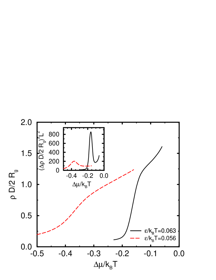
Figure 6: Adsorption isotherms slightly above the wetting transition temperature $\epsilon/k_{B}T_{\rm wet}=0.071$. The dependence of the layer thickness in units of the radius of gyration $\rho D/2R_{g}$ exhibits a turning point, indicative of a first order transition rounded by finite size effects. The inset presents the thickness fluctuations. From the location of the peak we have estimated the location of the prewetting line. Results are obtained via multihistogram analysis.

The determination of the complete phase diagram of a thick film in the MC simulations is beyond our computational facilities. However, we expect that the SCF calculations capture the qualitative behavior. To locate the prewetting line, we monitor the dependence of the layer thickness on the chemical potential for $k_{B}T/\epsilon=15.87=1.13k_{B}T_{\rm wet}/\epsilon$ and $k_{B}T/\epsilon=17.86=1.27k_{B}T_{\rm wet}/\epsilon$. We employ the system size $L=96$ and $D=80$. This technique has been employed previously by Pereira[22] and we use it in junction with a multi-histogram analysis[54] of our MC data. For large lateral extensions $L$, we expect a jump in the layer thickness $l$ and hysteresis at the (first order) prewetting transition. For $L=96$ however, a layer of thickness $R_{g}/2$ comprises only $\Phi L^{2}R_{g}/2N\approx 63$ polymers. Hence the prewetting transition is strongly rounded by finite size effects. The MC data are presented in Figure 6. The dependence of the layer thickness exhibits a turning point and from the corresponding maximum of the susceptibility we estimate the location of the prewetting line. Upon increasing the temperature the jump of the layer thickness decreases and the peak in the susceptibility becomes less pronounced. An accurate estimation of the prewetting critical point calls for a thorough finite size analysis, which is not attempted here. However, the data for the highest temperature are close to or above the prewetting critical temperature. Hence, the prewetting line is presumably less extended in the MC simulations than in the SCF calculations.

In a recent experiment, Zhao et al.[21] investigated the wetting properties of ultrathin polyethylene polypropylene (PEP) films on polished silicon wafers above the wetting temperature. These experiments reveal that slightly above the wetting temperature thick layers ($l\gg R_{g}$) wet the substrate, while ultrathin layers ($l<R_{g}$) break up into droplets and form pattern “analogous to those produced by spinodal decomposition”[21]. The layer thickness below which the layer dewets scales like the radius of gyration $R_{g}$. These findings were rationalized[21, 77] by the entropy costs of confining a chain into a layer which is thinner than the unperturbed chain extension. At higher temperatures, however, even ultrathin films of PEP wet the silicon waver.

This situation resembles the prewetting behavior: Slightly above the wetting transition two layers of different thickness $l_{-}$ and $l_{+}$ coexist. Since the length scale of the effective wall-interface interaction $g(l)$ scales like $R_{g}$, which is proportional to the correlation length of concentration fluctuations in the bulk and the characteristic decay lengths in the wings of the concentration profiles across an interface, so do the thicknesses of the coexisting layers. The reduction of the conformational entropy of the $A$ chains confined into an ultrathin layer is an important (though not unique) contribution to the effective wall-interface interaction $g(l)$ for $l<R_{g}$. A layer of thickness $l_{-}<l<l_{+}$ separates laterally into regions of thickness $l_{-}$ and $l_{+}$. If $\partial^{2}g/\partial l^{2}<0$ (cf. Figure 5 (a) inset) spinodal phase separation occurs, i.e. the layer is unstable against capillary fluctuations, which grow exponentially for large wavevectors in the early stage. Using the capillary fluctuation Hamiltonian (6), the fastest growing mode of the spinodal dewetting has the wavevector[78]

$$q^{*}=\sqrt{-\frac{1}{2\sigma}\frac{\partial^{2}g}{\partial l^{2}}}$$ (33)

Using the SCF results for our model in Figure 5 (a inset), we estimate $\partial^{2}g/\partial l^{2}\approx\gamma/2R_{g}\approx-0.00062k_{B}T$, $\sigma\approx 0.034k_{B}T$ and $q^{*}\approx 0.09=0.1\;\;2\pi/R_{g}$ close to the wetting transition. At temperature higher than the prewetting critical point however, there is no coexistence between thick and thin layers. Thus, $g(l)$ is convex for all thicknesses $l$ and ultrathin layers are stable. This temperature, chain length and layer thickness dependence and the concave curvature of the free energy, which leads to spinodal character of the dewetting, are compatible with the experimental findings[21].

To illustrate the dewetting of ultrathin polymer layers further, we perform MC simulations in the canonical ensemble, i.e. we let the chain conformations evolve via individual monomer hopping (LM) and slithering snake (SS) moves, however, identity switches $A\rightleftharpoons B$ are not allowed. Due to the slithering snake moves, we do not observe Rouse dynamics on short time and length scales, but the number of $A$-chains is conserved and we recover a purely diffusive dynamics on length scales larger than $R_{g}$. Of course, our MC simulation cannot reproduce fluid-like flow which is important for the late stage dynamics of spinodal decomposition[79]. Hence we do not attempt to relate our “MC time” to physical time units. Moreover, unlike the experimental situation, we consider a binary polymer melt in contact with a wall rather than a polymer solution. Long-ranged dispersion forces at the wall are not incorporated in our model. Due to the diffusive dynamics with conserved composition, the characteristic length scale $1/q^{*}$ being larger than the chain extension, and the universality of the wetting behavior we do expect, however, that the salient features of the early stage of phase separation are qualitatively captured in our MC simulations.

We study a cubic $123^{3}$ system. Initially both walls are covered with a flat, pure $A$-polymer layer of thickness $\langle l\rangle=4,8,16$, whereas the central portion of the film contains only B-polymers. In Figure 7 we display snapshots of the A monomers in the lower half of the container. Each $A$ monomer is presented as a sphere. The left row shows the time evolution of an ultrathin layer $\langle l\rangle=4=0.577R_{g}$ at $T=1.02T_{\rm wet}$. Initial concentration fluctuations grow rapidly. Later we observe A-rich domains which coarsen in time and in the last snapshots there is only one cluster which spans the whole system via the periodic boundaries in the lateral directions. The domain size is comparable with the extension of the container and no further domain growth takes place. Thus, we find clear evidence for dewetting in an ultrathin layer above the wetting temperature.

The time evolution of a thicker layer $\langle l\rangle=8=1.153R_{g}$ at the same temperature is presented in the middle row. Though we do observe some local thermal fluctuations of the $A$ concentration, the layer does not break up into domains. Thus, a thick layer does not dewet the walls at the same temperature[80]. To complete the analogy to the experiments we display the time sequence for a thin layer $\langle l\rangle=0.577R_{g}$ at $T=2.363T_{\rm wet}$. This temperature is above the SCF estimate of the prewetting critical temperature. Again we observe quite pronounced thermal lateral composition fluctuations on the length scale $R_{g}$. In the last snapshot an $A$-polymer has even escaped the layer. Note that at this temperature ($T=0.48T_{c}$) there is a small solubility of the $A$ component in the $B$ rich bulk. However, the length scale of composition fluctuations remains smaller than the box size. This indicates that the ultrathin layer is stable against spinodal dewetting at high temperatures.

This behavior can be quantified via a subbox analysis. We monitor the probability distribution $P(\nu)$ of the local $A$-monomer density $\nu$. For times larger than those displayed in the figures $P(\nu)$ is stationary, because if there is lateral phase separation the domain size has become comparable with the lateral system size. We average the lateral A-monomer density over square blocks of linear extension $B=1.154R_{g}$. The results of this analysis are presented in Figure 8. In (a) we study the dependence on the layer thickness $\langle l\rangle=\langle\nu\rangle/\Phi$ slightly above the wetting temperature $T=1.02T_{\rm wet}$. The layers of thickness $\langle l\rangle/R_{g}=1.154$ and $2.308$ exhibit a single peaked distribution centered around the initially homogeneous density. However, the thin layer $\langle l\rangle/R_{g}=0.577$ exhibits a bimodal distribution; one maximum is at $\nu=0$ and the other is located at $\nu/\Phi R_{g}\approx 0.8$. This double peak structure indicates the dewetting. The distribution for a thin layer at higher temperature $T=2.363T_{\rm wet}$ is also shown for comparison. It resembles the distribution of the thicker layers, just shifted to lower densities. Thus, the thin layer at higher temperatures is stable against spinodal dewetting. In Figure 8 (b) we present the temperature dependence of the subbox distribution as a function of the temperature. Upon reducing the temperature the distributions change very gradually from single peak to bimodal. The inset shows schematically the path along which we approach the coexistence between thick and thin layers. The solid curve is the result of our SCF calculations.

4.5 Interfacial profiles across the film

We proceed by exploring the detailed profiles across the film (i.e. perpendicular to the wall) and its dependence on the film width $D$ in the temperature regime between the critical temperature of the film and the wetting transition in the bulk. We choose $k_{B}T/\epsilon=50\approx 0.72k_{B}T_{c}/\epsilon$, which is far enough below the critical point to limit the influence of the shift of the critical temperature upon confinement and close enough to the critical point to obtain the preweighting factors of the composition within a small number of auxiliary simulations at intermediate temperatures. We study the wall separations $D=36,48,60,80,112$, which correspond to $D/R_{g}=5.2\cdots 16.2$. We employ a $96\times 96\times D$ geometry and for $D=48$ we gather some data for different lateral system sizes. The MC results are compiled in Tab. 2; effects of the varying the system size are small at this temperature.

Figure 9 presents the composition profiles $c(z)=\rho_{A}(z)/(\rho_{A}(z)+\rho_{B}(z))$ at coexistence, both in the MC simulations (a) and the SCF calculations (b). The profiles are symmetric about the middle of the film and only one half is displayed. Both methods yield qualitative similar results: Upon increasing the film width $D$, the coexistence potential approaches the bulk value and the thickness $l$ growths. This is qualitatively similar to complete wetting[4]. The surface order parameter and the width of the $AB$ interface increases with growing $D$ too. The profiles at the wall are flattened about the first $d$ lattice units in the simulations as well as in the SCF calculations.

The inset of Figure 9(a) displays the density profiles $\rho(z)$ for $D=60$, which exhibit pronounced packing effects. Also the results of the SCF calculations (not shown) exhibit some structure near the walls, however, the effect is much less pronounced than in the Monte Carlo simulations and the detailed packing structure is not reproduced by our SCF calculations. However, related SCF calculations of the surface segregation of a binary blend at a hard wall in the framework of an off-lattice model[81] achieve somewhat better agreement with MC simulations. Moreover, the width of the $AB$ interface is larger in the simulations than in the SCF calculations. This is partially due to broadening of capillary fluctuations and also expected because the distance to the critical point is smaller in the simulations than in the SCF framework. Moreover, the segregation in the middle of the film increases upon increasing the width of the film, whereas the opposite trend is observed in the SCF calculations.

The Figure 9 also shows the behavior of the parallel and perpendicular components of the end-to-end vector $\vec{R}$ as a function of its midpoint from the wall for $D=60$. The simulation data are presented in (c) and the SCF calculations in (d). At the wall, the perpendicular component $R_{\perp}$ vanishes for both components. Simulations and SCF calculations reveal that the parallel chain extension $R_{\|}$ of the A-component (majority) at the wall is larger than in the bulk. This transpires that the chains are not only deformed by the presence of the walls, but orient the long axis of their instantaneous shape parallel to the wall. Note that such an effect cannot be observed for Gaussian chains because the parallel and perpendicular extensions of Gaussian chains decouple completely and, hence, the parallel components of the chain extension are independent from the distance to the wall. The B-component (minority at the wall) shows hardly any deviation from its bulk value across the film in the MC simulations and in the SCF calculations.

Upon approaching the middle of the film simulations and SCF calculations show that the perpendicular extensions of A-chains attain their unperturbed value sooner than B-chains. The A-chains which are close to the $AB$ interface and in the minority (i.e. around z=20 and z=40) are stretched perpendicular to the $AB$ interface, as to reach with one end the corresponding A-rich layer close to the wall. Similar behavior is predicted for polymer/polymer interfaces[49], however, this effect cannot be resolved within the scatter of the simulation data. (Note that the concentration of A-chains is only $6\%$ in the middle of the film.) Furthermore we observe that the chain conformations at the AB interface are strongly affected by the presence of the wall. Thus, a film width of $D=48\approx 6.9R_{g}$ is not large enough to approximate the properties of the interfaces by their bulk behavior. At lower temperature, these deviations will become even more pronounced because the A-rich layer thickness decreases upon reducing the temperature.

We characterize the local structure of the polymeric fluid further by profiles of the intermolecular contacts across the film ($D=60$). The number of inter- and intramolecular contacts, without discrimination of the monomer species is presented in Figure 9 (e). In the middle of the film the number of intermolecular contacts $z$ is close to 2.65, the value used in the SCF calculations. In the vicinity of the wall the value decreases and exhibits pronounced oscillations. These characterize the local structure of the monomer fluid. As discussed in the previous section, they are indispensable for a quantitative prediction of the wetting behavior and surface thermodynamics. In the framework of our SCF calculations these “missing neighbors” at the wall are accounted for via a gradient expansion of the composition (cf. eq. (11))[55]. Though the SCF treatment captures the qualitative effects it cannot reproduce the detailed structure of the monomer fluid. The figure also displays the number of intramolecular contacts, which are assumed to be independent of the position in the SCF calculations. The number of intermolecular contacts of A-chains increases at the wall. A-chains try to bring many monomers close to the wall and adopt a flat (pancake-like) conformation which has a larger number of intermolecular contacts. This correlates with the increase of the perpendicular extension at the wall. The number of self-contacts of B-chains is reduced at the wall; B-chains try to escape the unfavorable monomer-wall interactions.

Measuring the number of intermolecular contacts between the same ($n_{AA},n_{BB}$) and unlike ($n_{AB}$) species, we can assess the validity of the random mixing assumption inherent in the SCF treatment.

$$\frac{2n_{AA}}{\Phi\rho_{A}^{2}}=\Phi\int_{r\leq\sqrt{6}}d^{3}r\;\;g_{AA}(r)\equiv z_{AA}\qquad\mbox{and}\qquad\frac{n_{AB}}{\Phi\rho_{A}\rho_{B}}=\Phi\int_{r\leq\sqrt{6}}d^{3}r\;\;g_{AB}(r)\equiv z_{AB}$$ (34)

$g_{IJ}$ denotes the intermolecular paircorrelation function, which is normalized such that $g_{IJ}(r\to\infty)=1$. The integration is extended over the spatial extension of the square well potential. For the temperature studied, we find quite pronounce deviations of our MC results from the random mixing assumption. The number of neighbors of the same species in the minority phase is strongly enhanced. This indicates a clustering of chains in the minority phase, similar to the observation of composition fluctuations in the ultrathin film at $\epsilon/k_{B}T=0.03$ shown in Figure 7. This non-random mixing also correlates with the underestimation of the composition of the minority component (cf. Figures 4 (a,c)). For the temperature studied, the mean field approximation underestimates the bulk minority composition $\langle\rho\rangle$ by a factor 0.68. Increasing the chain length, however, we can reduce these local composition fluctuations and we find random mixing behavior for very long chains[46] in accord with the Ginzburg criterion[83].

4.6 Dependence on the film width: Kelvin equation

We analyze the dependence of the layer thickness and the coexistence chemical potential on the film thickness. This yields information about the strength and spatial range $1/\lambda$ of the interaction $g(l)$ between the wall and the $AB$ interface at a distance $l$ from the wall. The shift of the coexistence chemical potential $\Delta\mu_{\rm coex}$ with the film width $D$ is displayed in Figure 10 (a) for the simulations and the SCF calculations. The straight line depicts the leading finite size behavior according to eq. (5), where we have used the independently determined interfacial tension[47] and have estimated the width $l$ of the A-rich layers as in section (A). The phenomenological treatment describes the data very well. Only for the smallest system sizes there are some deviations, which are more pronounced for the simulation data. From the next-to-leading order corrections we can roughly estimate the spatial range of the effective interaction between the wall and the $AB$ interface, albeit with large uncertainties: $1/\lambda_{\rm MC}\approx 7$ and $1/\lambda_{\rm SCF}\approx 6.2$. Note that these length scales are much larger than the range $d=2$ over which microscopic monomer-wall interactions $\epsilon_{w}$ are extended in our model.

The increase of the width $l$ of the A-rich layers upon approaching the bulk coexistence chemical potential is presented in Figure 10 (b) for the simulations and the SCF calculations. The behavior for large wall separations $D$ is well described by eq. (4) and the slope of $l$ vs. $\ln(-\Delta\mu_{\rm coex})$ yields an estimate for the range $1/\lambda$ of the wall-interface potential. Again, we find deviations for small values of $D$ from the anticipated behavior.

To explore the effect of the confinement in more detail, we investigate the profiles in the SCF framework. Figure 11 displays the composition profiles of the unconfined interface and the interface in a film of width $D=49$ on a logarithmic scale. The solid line represents a tanh profile with width $w=6.91$ which describes the SCF result at the center of the profiles. However, there are deviations in the wings of the profiles. There the length scale of the exponential decay is set by the correlation length $\xi$[40]. The interfacial profile in the thin film is narrower and decays more rapidly. To quantify this effect, we use the gradient of the composition profile and define an effective tension via $\Sigma/k_{B}T\sim\Phi b^{2}\int dz\left(\frac{\partial c}{\partial z}\right)^{2}$. This expression yields the correct interfacial tension in the weak segregation limit, and we expect to obtain qualitatively reasonable results also for the temperature studied here. The ratio between this tension and the corresponding bulk quantity is shown in the inset as a function of the thickness of the wetting layer $l$. The effective tension is clearly position dependent, and increases upon confinement. The right inset presents the wall-interface potential g(l) as a function of the thickness of the wetting layer $l$ for $D=49$. The data are describable by an exponential decay with length scale $1/\lambda=4.33$. Using eq. (8) we extract a parallel correlation length $\xi_{\|}\sqrt{\sigma_{AB}/\sigma}\approx 43$ ($\sigma_{AB}$: bulk interfacial tension, $\sigma$ “effective” interfacial tension in the capillary fluctuation Hamiltonian).

As noted in Figure 2 (a), the composition fluctuations in the A-rich phase are larger than in the phase without interfaces. This is caused by fluctuations of the average interfacial position $l$. Assuming that the fluctuations at both walls are independent, we can relate the excess composition fluctuations to the fluctuations of the layer thickness:

$$\langle\Delta\rho^{2}\rangle_{\rm excess}=\frac{\chi_{-}-\chi_{+}}{L^{2}D}=\frac{2}{D^{2}}(2\langle\rho\rangle-1)^{2}\langle\delta l^{2}\rangle$$ (35)

where $\chi_{\pm}$ are the susceptibility in the A-rich and A-poor phases, respectively. Using $L^{2}\langle\delta l^{2}\rangle=\left(\frac{\partial^{2}g}{\partial l^{2}}\right)^{-1}$ and eq. (4), we can estimate the interaction range $1/\lambda$ and parallel correlation length $\xi_{\|}$ from a single simulation via:

$$\frac{1}{\lambda}=\frac{\Phi}{2N(2\langle\rho\rangle-1)}D\Delta\mu_{\rm coex}\;DL^{2}\langle\Delta\rho^{2}\rangle_{\rm excess}\qquad\mbox{and}\qquad\frac{\xi_{\|}^{2}}{\sigma}=\frac{\pi L^{2}D^{2}}{(2\langle\rho\rangle-1)^{2}}\langle\Delta\rho^{2}\rangle_{\rm excess}$$ (36)

The estimates for the parallel correlation length are compiled in Tab. 2. $\xi_{\|}$ increases with the film width $D$ and is always smaller than our lateral system extension $L$. However, this method entails rather large uncertainties and a direct measurement[41] would yield more reliable estimates.

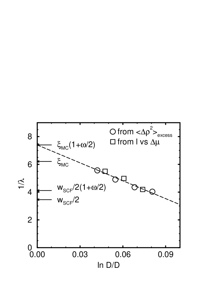
Figure 12: Effective interaction range of the interface-wall potential extracted from the Monte Carlo data. The circles are estimates according to eq. (35), the squares correspond to the slope of thickness $l$ of the wetting layer vs the logarithm of the coexistence potential $\Delta\mu$. The arrows denote possible limiting values for the interaction range.

The dependence of the effective interaction range on the width of the film is presented in Figure 12. The data are compared with the local slope $dl/d\ln(-\Delta\mu_{\rm coex})$. Both estimates are consistent, which reveals that the excess composition fluctuations are indeed due to fluctuations of the average wetting layer thickness. Upon increasing the film width $D$, the effective interaction range increases. Therefore, the wall-interface interaction is not a simple exponential repulsion. Assuming that the deviations from the large $D$ behavior are of the form $\ln D/D\sim l\exp(-\lambda l)$, the interaction range approaches a value $1/\lambda\approx 7.4(6)=6.2(5)(1+\omega/2)$, where we have used the MC results for the interfacial tension and the bulk correlation length (cf. Tab. 2) at $k_{B}T/\epsilon=0.02$ to estimate $\omega\approx 0.382$. Assuming a $1/D$ correction (not shown), we obtain a slightly smaller value $\lambda\approx 6.8$ as estimate for large $D$. Thus $1/\lambda(1+\omega/2)$ is of the same order as the correlation length of composition fluctuations $\xi_{\rm MC}=6.21$ in the bulk, but somewhat smaller than the intrinsic interfacial width $w_{\rm SCF}/2\approx 3.5$ (as extracted from the SCF calculations). Thus Figure 12 yields tentative evidence for the suggestion [43] that $1/\lambda=\xi(1+\omega/2)$ indeed is relevant, corroborating recent studies of Ising models[82].

4.7 Interfacial fluctuations

The behavior of the fluctuating $AB$ interface, which is bound to the wall, can be described via an effective Hamiltonian. Much theoretical investigations have been directed towards the detailed form of this Hamiltonian[43, 84]. In its simplest form (cf. eq. (6)) this Hamiltonian comprises a contribution from the increase of the interfacial area due to deviations $\delta l$ of the local interface position from its average value $\langle l\rangle$ and an effective wall-interface potential $g(l)$. Since the $AB$ interface is distorted by the presence of the wall (cf. Figure 11), the range of the wall-interfacial interaction depends on the thickness of the wetting layer $\langle l\rangle$. A similar dependence is expected for the effective interfacial tension $\sigma$[43, 84].

The effective interfacial tension $\sigma$ can be accurately measured in the MC simulations via the spectrum of capillary fluctuations[34, 35]. Unlike previous studies[34, 35] we use an integral criterion[41] for the local y-averaged interfacial position:

$$l(x)=\frac{\int_{0}^{D/2}dz\;\int dy\;\;\rho_{A}(x,y,z)}{\frac{2}{D}(2\langle\rho\rangle-1)\int_{0}^{D/2}dz\;\int dy\;\;\left(\rho_{A}(x,y,z)+\rho_{B}(x,y,z)\right)}+\mbox{const}$$ (37)

The local interfacial position can be Fourier decomposed according to

$$l(x)\sim\frac{a_{0}}{2}+\sum_{k=0}^{L/2-1}\Big{[}a(q_{k})\cos(q_{k}x)+b(q_{k})\sin(q_{k}x)\Big{]}$$ (38)

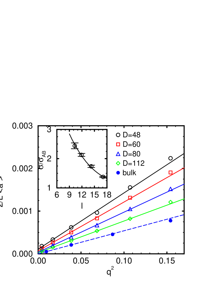
Figure 13: Fluctuation spectrum of the AB-interface for different system sizes $D$. The solid lines corresponds to fits in the range $0<q^{2}<0.12$. The dashed line corresponds to the capillary fluctuations with $\sigma_{AB}=0.054$, the value measured independently via reweighting techniques. The filled circles represent the capillary fluctuation spectrum in the bulk system ($64\times 64\times 128$ geometry and periodic boundary conditions). The inset shows the ratio of the effective interfacial tension and its bulk value on the thickness $l$ of the wetting layer. The solid line corresponds to $\sigma/\sigma_{AB}=1+8.72(0.272l)\exp(-0.272l)$.

with $q_{k}=2\pi k/L$. Using the equipartition theorem, we find that the Fourier amplitudes are Gaussian distributed and their variances are given by eq. (7). Previous simulations of unconfined interfaces[34, 35] have shown that the Fourier amplitudes are indeed Gaussian distributed and that $\sigma$ can be identified with the interfacial tension $\sigma_{AB}$, which has been measured independently. In the present simulation we verify this again for temperatures closer to the critical point. The full circles in Figure 13 display the spectrum of interfacial fluctuations of the unconfined interface (using a local criterion for the interfacial position[35]), whereas the dashed curve corresponds to the prediction (7) with $g=0$ and $\sigma=\sigma_{AB}$ as determined independently via a reweighting technique.

The results for the confined system are presented in Figure 13. The open symbols denote the simulation data, whereas the solid lines present linear regressions according to eq. (7). The fit yields the parallel correlation length $\xi_{\|}$ and the effective interfacial tension $\sigma$. Unfortunately, the integral definition of the local interface position is affected by bulk composition fluctuations, which result in an overestimation of the fluctuations of the local interfacial position. However, assuming that these bulk composition fluctuations are laterally uncorrelated on length scales $2\pi/q$ larger than the bulk correlation length $\xi$, we can taken them into account by the substitution:

$$\left(\frac{\partial^{2}g}{\partial l^{2}}\right)_{\rm eff}^{-1}\approx\left(\frac{\partial^{2}g}{\partial l^{2}}\right)^{-1}+\frac{D\chi_{+}}{2(2\langle\rho\rangle-1)^{2}}$$ (39)

where $\chi_{+}$ is the susceptibility of the A-rich phase. Using $\langle a_{0}^{2}\rangle=\frac{4}{L^{2}}(\frac{\partial^{2}g}{\partial l^{2}})^{-1}$ and $a_{0}=\frac{2}{L}\int dx\;l(x)$, we rederive eq. (35). Thus, bulk composition fluctuations mainly influence our estimate of $\xi_{\|}$. However, we can still use eq. (7) to extract an effective interfacial tension $\sigma$ for $0<q<2\pi/\xi$.

Most notably, the effective interfacial tension for width $D=48\approx 6.9R_{g}$ is more than twice as large as in the unconfined system. The thickness dependence of the effective interfacial tension is presented in the inset of Figure 13. The additional contribution to the interfacial tension is well describable by the predicted form[43, 84] $\Delta\sigma\sim l\exp(-\lambda l)$ and the fitting parameter $1/\lambda\approx 3.7$ is roughly compatible with the previous estimates for the effective interaction range for small $l$. Moreover, this effect is also born out in the SCF field calculations. As presented in Figure 9(b) and Figure 11, the interfacial width in the confined geometry is slightly smaller and the effective interfacial tension is larger than in the bulk. The absolute magnitude of this effect in the SCF calculations is however somewhat smaller than in the MC simulations.

5 Summary and discussion

We have presented a comparison between extensive MC simulations and SCF calculations on the phase behavior of a binary polymer blend which is confined into a film of width $D$. The hard walls at the film boundaries are ideally flat and preferentially absorb the A-component of the mixture via a short range interaction. Combining simulations in the semi-grandcanonical ensemble with reweighting techniques[52, 53], we accurately determine the phase diagram of the confined blend and the shift of the coexistence chemical potential. The critical point is shifted to lower temperatures and higher concentrations of the A-component. At the vicinity of the critical point 2D Ising-like critical behavior is observed in the MC simulations, in agreement with previous simulations by Rouault et al. [24] on confined blends between “neutral” walls. The binodals of the confined blend are asymmetric. The A-poor binodal is convex in an intermediate temperature regime. This curvature is the signature of the wetting transition in the semi-infinite system. Also the temperature dependence of the coexistence chemical potential changes around the wetting temperature.

Using a novel extended ensemble which allows the monomer-wall interaction to fluctuate we accurately locate the wetting transition in the MC simulations according to the Young equation. Simulations and SCF calculations reveal that the film width $D$ gives rise to a pronounced rounding and shift of the wetting transition. We find evidence for a first order wetting transition at rather low temperatures $T_{\rm wet}\approx 0.2T_{c}$. This is also in agreement with our SCF field calculations. In the limit of a strong first order transition the wetting temperature is inversely proportional to the square of the integrated monomer-wall interaction strength and independent of the chain length $N$. We cannot rule out that critical wetting occurs in the ultimate vicinity of the critical point. However, for all parameters investigated, we find only first order wetting transitions in our simulations.

We determine the prewetting line, at which a thin and a thick wetting layer coexist, in the SCF calculations and estimate its location in our MC simulations. We suggest that recent experiments of Zhao and co-workers[21] on the spinodal dewetting of ultrathin polymer films can be analyzed in terms of spinodal phase separation into a thin and a thick wetting layer. The chain length and temperature dependence of the prewetting is in agreement with the experimental observations. The results are further illustrated by a MC study of the early stage of spinodal dewetting.

The dependence of the coexistence chemical potential on the film width is well describable by a Kelvin equation[12] for large $D$. The leading behavior is quantitatively predicted by the phenomenological description. The increase of the thickness $l$ of the wetting layer is compatible with a logarithmic dependence on the film width or the coexistence chemical potential. Using the size dependence of the wetting layer thickness or the excess composition fluctuations of the A-poor phase, we measure the effective wall-interface interaction range $1/\lambda$. Our results are compatible with the prediction of Ref. [43] $1/\lambda=\xi(1+\omega/2)$, where $\xi$ is the bulk correlation length which set the length scale in the wings of the interfacial profile[40] and $\omega$ is the wetting parameter.

The surfaces give rise to a pronounced orientation of the end-to-end vector. Both our SCF calculations, and MC simulations show an increase of the lateral chain extension at the wall, whereas the z-extension vanishes at the wall. The length scale of orientation is set by the radius of gyration. Even for large wall separations $D\approx 20R_{g}$, the conformations at the $AB$ interface are perturbed. We find that the interfacial width of the confined $AB$ interface is smaller than in the bulk and approaches gradually the bulk value for very large $D$.

We determine the local (laterally resolved) position of the $AB$ interface bound to the wall. Analyzing the spectrum of capillary fluctuations[34, 35] of the bound interface, we determine the position dependence of the interfacial tension. The effective interfacial tension is compatible with the predicted form $\sigma-\sigma_{AB}\sim l\exp(-\lambda l)$[43, 84]. In the film of width $D=48\approx 6.9R_{g}$, the effective tension $\sigma$ exceeds the bulk value $\sigma_{AB}$ by more than a factor of 2. This increase is due to a deformation of the interfacial profile near the wall, which is also observed in the SCF calculations.

The chain length dependence of our results is not addressed in the simulations; we consider only polymers consisting of N=32 coarse grained monomers. This corresponds to rather short polymers of about 150 chemical repeat units. Let us briefly comment on the behavior of longer chains: The length scale of the wetting layer, the range of the effective wall-interfacial interaction and the correlation length in the bulk is set by the radius of gyration $R_{g}\sim\sqrt{N}$. The phase behavior in the bulk is characterized by the interaction strength per polymer $\chi N$. However, if the preferential interactions of the monomers with the wall $\epsilon_{w}$ are chain length independent, the wetting temperature is also independent of the molecular weight. Thus wetting in blends of high molecular weight occurs far away from criticality and is generically of first order.

Our SCF calculations incorporates the detailed chain conformations on all length scales without any adjustable parameter. They qualitatively describe a variety of different MC results on polymer blends in thin films; for some properties nearly quantitative agreement is achieved. Moreover, the SCF calculations are at least an order of magnitude less computational intense than the MC simulations. They are useful to extend the MC results to larger film width, where we find a triple point at which a thin and a thick wetting layer coexist with an $A$-rich bulk. However, there are qualitative deviations in the behavior around the critical point, and the SCF calculations quantitatively underestimate the thickness of the wetting layer and overestimates the wetting transition. We discuss them in turn:

A) In the vicinity of the critical temperature, the mean field treatment fails to describe the shape of the binodal which is characterized by Ising critical behavior. Thus the binodals are flatter in the MC simulations than in the SCF calculations and the critical temperature is overestimated by the SCF calculations. According to the Ginzburg criterion[83] we expect that in 3D the mean field behavior extends the closer to the critical point the longer the chain length is. Simulations[46] in 3D confirm that the Flory-Huggins theory describes the behavior correctly in the limit $N\to\infty$. Hence SCF calculations and MC simulations agree better for higher molecular weight blends. We expect this also to hold true in the confined geometry. Though the system exhibits 2D Ising critical behavior, the polymer conformations are not flat pancakes but interpenetrate and hence interact with many neighbors. The asymptotic critical behavior of Ising type is observed if the correlation length $\xi$ exceeds a crossover length scale $\xi_{\rm cross}\sim N$ [32], and depending whether $D>\xi_{\rm cross}$ or $D<\xi_{\rm cross}$ different scenarios apply.

B) Moreover, the mean field treatment neglects capillary fluctuations. These lead to a pronounced broadening of the apparent interfacial width[41] that persists even for very long chain lengths. They also increase the effective wall-interface interaction range. Our present simulations and previous studies[41] are consistent with the prediction[43] that the interaction range is amplified by a factor $(1+\omega/2)$, where $\omega=k_{B}T/4\pi\xi^{2}\sigma_{AB}$ denotes the wetting parameter. Thus the SCF calculation underestimates the thickness of the wetting layers, in agreement with our comparison. However, at constant $\chi N$, the interfacial tension decreases like $1/\sqrt{N}$ whereas the correlation length $\xi$ is of the size of the polymer extension $\sqrt{N}$. Thus the wetting parameter $\omega$ decreases like $1/\sqrt{N}$ at fixed $\chi N$ and we expect that the concomitant underestimation of the wetting layer thickness becomes smaller upon increasing the chain length, at least for temperatures not too far from the critical point where the above formula for $\omega$ applies.

C) Another important source of discrepancies between SCF calculations and the MC results in the long chain limit is the treatment of the local structure of the fluid at the wall. Our SCF calculations incorporates the detailed chain structure on all length scales, uses the same monomer-wall interactions as the simulations, and accounts of the finite compressibility of the melt. In the present calculations, however, the reduction of the number of intermolecular interactions due to the presence of the wall (“missing neighbor effect”) is only qualitatively treated via a gradient expansion of the segmental energy density[55]. The pronounced packing effects at the wall are not quantitatively captured by our SCF calculations. These effects plays a crucial role for a quantitative prediction of the wetting behavior (cf. eq. (31) and (25)). There are attempts to incorporate the local structure of the fluid at the wall into the SCF framework. Nath et al.[28] incorporated fluid packing via the direct correlation function of the liquid. This quantity can be determined independently via P-RISM integral and/or density functional theory. In addition the polymers deform at the vicinity of the walls. The conformational changes alter the number of intermolecular and intramolecular contacts. These effects depend on the molecular architecture of the polymers and on the detailed structure (e.g. corrugation potential, microscopic roughness) of the wall. E.g. structural asymmetries between the components may give rise to entropic contributions to the spreading parameter. We anticipate that these will be important for polymer-solvent systems in contact with a wall. A proper treatment of these effects is out of the scope of the present study which is focussed on the universal polymeric behavior of confined binary melts.

Acknowledgment

It is a great pleasure to thank J. Baschnagel, F. Schmid, Y. Rouault, and A. Werner for helpful discussions. The generous allocation of about $10^{5}$ hours of single processor CPU time on the CRAY T3E at the HLRZ Jülich and the CONVEX SPP2000 at the computing center Mainz is grateful acknowledged. This work was supported by BMBF grant No. 03N8008C and DFG grant Bi314/17.

Appendix: Composition dependence of the free energy in the thin film near the wetting transition

The free energy $F$ as a function of the composition $\rho$ is accessible in the simulations via the probability distribution $P(\rho)$: $F(\rho)/k_{B}T\sim-\ln(P(\rho))$. The MC results for system geometry $48\times 48\times 48$ in the vicinity of the wetting transition of the semi-infinite system ($\epsilon/k_{B}T=0.07$, $\epsilon_{w}/k_{B}T=0.0695$, $\Delta\mu=0$) are presented in Figure 5. Unlike the SCF calculations, the composition in the simulation is not necessarily laterally homogeneous nor symmetric around the middle of the film. Rather the system chooses a configuration which minimizes the free energy at fixed overall composition. We can estimate the relative stability of the different conformations by some simple free energy considerations[2, 85].

If the lateral system extension $L$ is large, the systems will phase separate laterally into A-rich and B-rich domains. Those domains are separated via two interfaces, which run perpendicular to the walls For simplicity we approximate the free energy costs of these perpendicular interfaces by $\sigma_{AB}(D-2l)L$ and assume that $\Delta\sigma_{\rm w}\approx\sigma_{AB}\ll\gamma$, i.e., the thickness of the wetting layer $l$ is allowed to adjust as to minimize the overall free energy. The excess free energy of such a configuration is given by:

$$\Delta F=\min_{\alpha}\left(\alpha 2L^{2}\sigma_{AB}+2L(D-2l)\Delta\sigma_{\rm w}\right)\qquad\mbox{with}\qquad DL\frac{\langle\rho\rangle-\rho}{2\langle\rho\rangle-1}=\alpha L(D-2l)$$ (40)

Minimization leads to $\Delta F=4L\sqrt{\sigma_{AB}\Delta\sigma_{\rm w}DL{[\langle\rho\rangle-\rho]}/{[2\langle\rho\rangle-1]}}$. Comparing this result to the lateral homogeneous situation $\Delta F=2L^{2}\sigma_{AB}$ (independent of $\rho$), we find that for ${[\langle\rho\rangle-\rho]}/{[2\langle\rho\rangle-1]}<\Delta\sigma_{\rm w}L/4D\sigma_{AB}$ lateral phase separation occurs. Indeed for $\rho>0.7$ the excess free energy in the simulations decreases strongly and upon approaching $\rho=1$ the two interfaces annihilate.

For small compositions $\rho$, no lateral phase separation occurs. However, unlike the situation in the SCF calculations, the thickness of the wetting layers $l_{r},l_{l}$ on both sides need not to be identical; only the average thickness $\bar{l}=\frac{l_{r}+l_{l}}{2}=\frac{D(\rho-\langle\rho\rangle+1)}{2(2\langle\rho\rangle-1)}$ is fixed by the constraint on $\rho$. Let $g(l)L^{2}$ denote the potential of a single interface at a distance $l$ from the wall. Then the excess free energy of the system with two interfaces is given by: $\Delta F/L^{2}=\min_{\Delta l}\left((g(\bar{l}+\Delta l)+g(\bar{l}-\Delta l)\right)$. If the wetting transition is first order, than $g(l)$ has a minimum $g(l_{0})=0$ at a finite distance from the wall, is convex around its maximum of height $\gamma$, and vanishes for large $l$. For $\bar{l}$ around the maximum, the system chooses rather $l_{l}\approx l_{0}$ and $l_{r}\approx 2\bar{l}-l_{0}$ than $l_{l}=l_{r}=\bar{l}$ which yields $\Delta F/2L^{2}\approx g(l^{*})/2$ with $l^{*}=2\bar{l}-l_{0}$[86]. Therefore, the hump in the free energy corresponds to a conformation in which one interface is at $l_{0}$ (“dry” state) and the height of the hump is $\gamma L^{2}$. If one allows for lateral variation of the wetting layer thickness, the hump in the free energy can be reduced further to $O(1/L)$. We expect that the maximum of the free energy is shifted to smaller values of the composition and its height is at most $\gamma$, i.e., half the value in the SCF calculations. From the probability distribution $P(\rho)$ we can estimate the free energy $\gamma$, which controls the lifetime of the “dry” state. Using the simulation data in Figure 5, we obtain the rough estimate $\gamma/k_{B}T>0.0019(10)$ at $\epsilon/k_{B}T=0.0695$. Gratifyingly, this is of the same order of magnitude as the mean field result $\gamma/k_{B}T=0.0027(8)$ at $\epsilon/k_{B}T=0.0575$

	$k_{B}T_{c}^{\rm bulk}/\epsilon$	$k_{B}T_{c}/\epsilon$	$k_{B}T_{\rm wet}/\epsilon$	$\rho_{c}$	$\sigma(k_{B}T/\epsilon=50)/k_{B}T$	$\rho(k_{B}T/\epsilon=50)$	$w(k_{B}T/\epsilon=50)$	$\xi(k_{B}T/\epsilon=50)$
MC	69.3(3)	55.5(6)	14.1(7)	0.686(5)	0.0054(1)	0.9369	10.71	6.21
SCF	84.8	76.7	17.2	0.69	0.0075	0.9569	6.91	4.72

Table 1: Bulk properties as measured in the Monte Carlo simulations and self-consistent field calculations. Length scales are measured in units of the lattice spacing $u$, and the interfacial tension in units of $k_{B}T/u^{2}$. The interfacial width in the Monte Carlo simulations includes additional broadening due to capillary waves ($L=64$), whereas the SCF result refers to the intrinsic width. The mean field correlation length is given by $\xi=\frac{R_{g}}{\left(3(1-2\chi N\rho(1-\rho)\right)^{1/2}}$ with $\chi=2{\tt z}\epsilon/k_{B}T$

$D$	$\Delta\mu/k_{B}T$	$\rho_{-}$ (B-rich)	$\rho_{+}$ (A-rich)	$l$	$\xi_{\|}(\sigma_{AB}/\sigma)^{1/2}$	$\sigma/k_{B}T$
36	-0.6575	0.5096	0.8605	9.20	11.3
48	-0.3944	0.4376	0.9185	10.29	14.3	0.0133(4)
48∗	-0.3937	0.4379	0.9187	10.29
48†	-0.3938	0.4421	0.9143	10.41
60	-0.2682	0.4097	0.9301	11.90	18.0	0.0115(2)
80	-0.1670	0.3747	0.9359	14.26	24.2	0.0094(2)
112	-0.0996	0.3300	0.9381	17.10	33.3	0.0074(1)
$\infty$	0	0.0631	0.9369	$\infty$	$\infty$	0.0054(1)

Table 2: Simulation data for $\epsilon=0.02,\epsilon_{\rm w}=0.16$ and lateral system size $L=96$ (if not indicated otherwise: ^∗ $L=160$, ^† $L_{x}=164\times L_{y}=48\times D=48$). The errors for the coexistence value of the chemical potential difference $\Delta\mu$ are less than 1$\%$, the uncertainties for the coexistence composition are $2\%$ for the B-rich phase and $1\%$ for the A-rich phase. The errors of the effective interfacial tension are extracted from the regression of the simulation data in Figure 12.

$D$	$\Delta\mu/k_{B}T$	$\rho_{-}$ (B-rich)	$\rho_{+}$ (A-rich)	$l$
37	-0.6182	0.381	0.948	6.84
49	-0.3875	0.356	0.954	8.39
61	-0.2764	0.338	0.956	9.84
81	-0.1803	0.302	0.958	11.47
113	-0.1134	0.258	0.958	13.29
137	-0.0874	0.233	0.957	14.22

Table 3: Results of the self-consistent field calculations for the same interaction strength $\epsilon/k_{B}T=0.02,\epsilon_{\rm w}/k_{B}T=0.16$ as the Monte Carlo simulation.

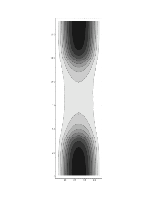
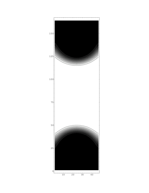
Figure 1: 2D composition profiles in a $164\times 48\times 48$ geometry. $B$ rich regions are shaded darker. The walls attract the $A$ component ($\epsilon_{w}/k_{B}T=0.16$).
(a) $\epsilon/k_{B}T=0.02$ (above the wetting temperature) and average A-monomer density $\langle\rho\rangle=0.67751$.
(b) $\epsilon/k_{B}T=0.08$ (below the wetting temperature) and average A-monomer density $\langle\rho\rangle=0.5$.

         

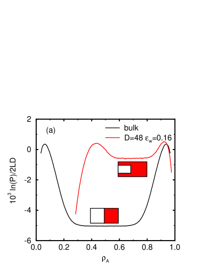
Figure 2: (a) Probability distribution of the composition at $\epsilon/k_{B}T=0.02$ for the bulk system ($L_{x}=128\times L=64\times D=64$ and periodic boundary conditions in all directions) and the confined system ($L_{x}=164\times L=48\times D=48$, $\epsilon_{\rm w}/k_{B}T=0.16$). The peaks correspond to the coexisting phases and have equal probability weight. The typical configurations of the plateau between the two peaks contain two interfaces parallel to the $yz$-plane (as sketched). The detailed composition profile of the confined blend is displayed in Fig. 1 (a).
(b) Temperature dependence of the line tension $\Gamma$ between the coexisting phases in a thin film $D=48$. The Flory–Huggins parameter is given by $\chi={2{\tt z}\epsilon}/{k_{B}T}$, with the intermolecular coordination number ${\tt z}=2.65$.
The inset shows the ratio between the line tension and the bulk interfacial tension as a function of the inverse temperature.

         

         

         

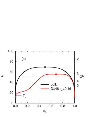
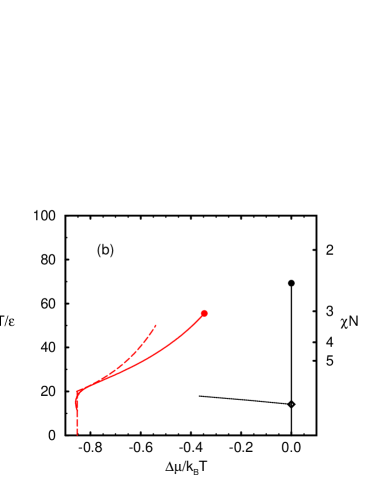
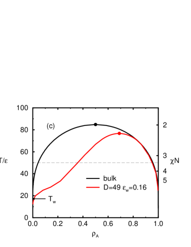
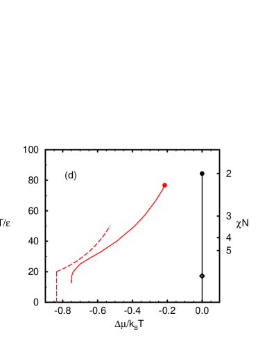
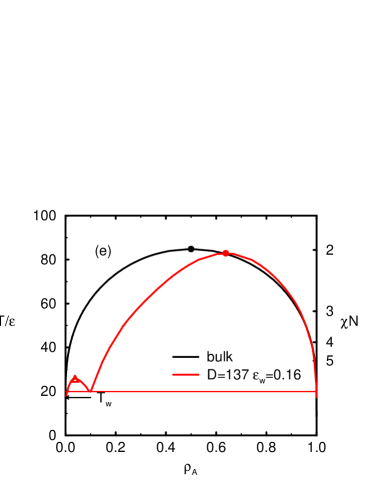
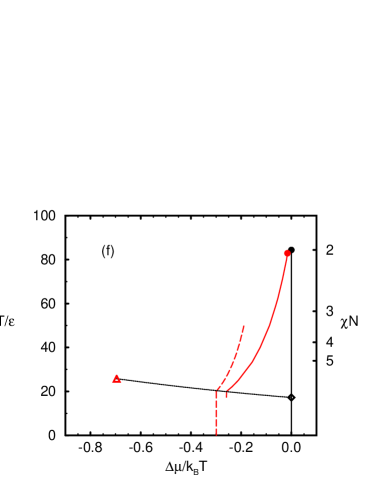
Figure 4: Comparison of the MC phase diagrams and the SCF results:
(a) MC results for the phase diagram in the bulk and confined geometry ($D=48$ and $\epsilon_{\rm w}/k_{B}T=0.16$). The critical points exhibit 3D and 2D Ising critical behavior. The estimate for the wetting temperature is indicated by an arrow. The dashed line marks the temperature at which the thickness dependence is investigated.
(b) MC results for the coexistence chemical potential difference $\Delta\mu$. The dashed lines correspond to the low temperature estimates $-\Delta\mu D/k_{B}T=2Nb({\chi/6})^{1/2}$ and $-\Delta\mu D/k_{B}T=4dN\epsilon_{w}/k_{B}T$. The wetting transition in the semi-infinite system is denoted by an diamond. The dotted line presents our estimate for the prewetting line (and its continuation above the prewetting critical temperature).
(c) Phase diagram according to the SCF calculations (symbols as in (a)) for $D=49$.
(d) Phase diagram in the $T-\Delta\mu$ plane according to the SCF calculations (symbols as in (b)).
(e) Phase diagram in the SCF calculations for a thick film $D=137$. Slightly above the wetting temperature there is a triple point (horizontal solid line) at which a thin layer, a thick layer, and an $A$-rich phase coexist. The coexistence between layers of different thicknesses ends at a tricritical point denoted by a triangle.
(f) Phase diagram in the $T-\Delta\mu$ plane according to the SCF calculations for $D=137$ (symbols as in (b)) The diagram also includes the prewetting line (calculated from a film of width $D=137$).

                             

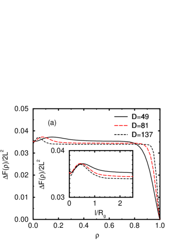
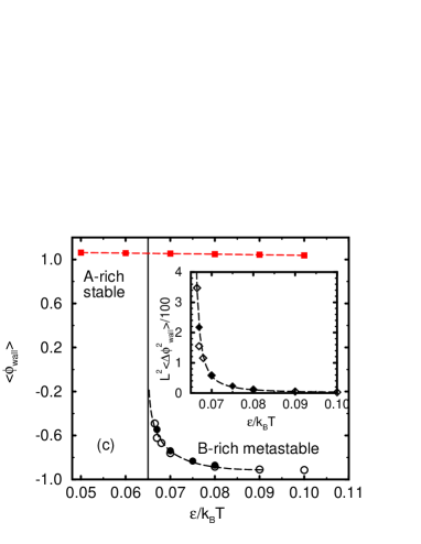
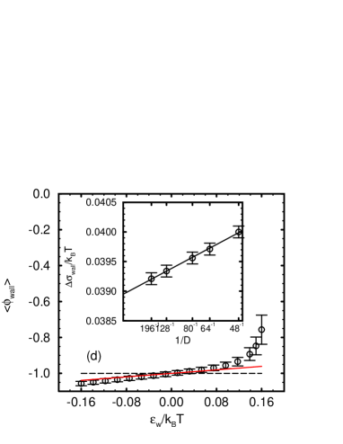
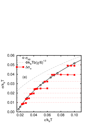
Figure 5: Locating the wetting transition:
(a) Mean field free energy at $\epsilon/k_{B}T=0.0575$ for different film thicknesses $D$. The inset presents the same data vs the ratio of the thickness of the wetting layer $l=\rho D/2$ and the chain extension $R_{g}$.
(b) Probability distribution of the composition at $\epsilon/k_{B}T=0.0695$ in a cubic $48^{3}$ container. The horizontal dashed line marks the bulk interfacial tension $\sigma_{AB}=0.0387k_{B}T$ at this temperature. The inset presents the probability distribution for small A contents at different temperatures.
(c) Surface order parameter $\phi_{\rm wall}$ and surface layer susceptibility as a function of temperature for fixed $\epsilon_{\rm w}=0.16$ at the bulk coexistence chemical potential difference $\Delta\mu=0$. Open symbols represent the simulation data for $L=96$ and $D=80$, whereas filled symbols refer to $L=D=128$. Lines are only guides to the eye. Around $\epsilon=0.065(3)$ we find evidence for a wetting spinodal.
(d) Surface order parameter as a function of the monomer-wall interaction strength $\epsilon_{w}$ at fixed $\epsilon/k_{B}T=0.07$. The bars do not represent statistical errors but the variance of the distribution of $\phi_{\rm wall}$. The horizontal dashed line shows the naive estimates in the strong segregation limit, whereas the solid lines takes account of compressibility effects. The inset displays the dependence of $\Delta\sigma_{\rm wall}$ on the film width $D$.
(e) Interfacial tension $\sigma_{AB}$ and wall free energy difference $\Delta\sigma_{\rm w}$ as a function of the interaction strength $\epsilon$. Symbols denote results of the Monte Carlo simulations. Horizontal dashed lines present our estimate in the strong segregation limit (SSL). The dashed line displays the low temperature estimate of the interfacial tension, whereas the solid line $\sigma/k_{B}T=0.1792(\epsilon/k_{B}T)^{1/2}\left(1.126-0.0222/(\epsilon/k_{B}T)+8.04\;10^{-5}/(\epsilon/k_{B}T)^{2}\right)$ shows a fit to the MC data.
(f) Dependence of the inverse wetting temperature $\chi_{\rm wet}$ on the monomer-wall interaction strength $\epsilon_{w}$. circles denote our MC estimates, the solid line shows the behavior in the strong segregation limit for infinite chain length, whereas the dashed line incorporates the effect of finite chain length on the bulk interfacial tension to first order in $1/\chi N$.

figures available upon request

Figure 7: Configuration snapshots of dewetting in thin polymer layers. The left row of snapshots displays the spinodal dewetting process in an ultrathin polymer layer above the first order wetting transition ($\epsilon/k_{B}T=0.0695$). The middle row presents the behavior of a thicker layer at the same temperature; the layer remains stable. The right sequence shows the behavior of the thin layer above the prewetting critical temperature ($\epsilon/k_{B}T=0.03$). The layer does not dewet; however there are strong thermal fluctuations.

         

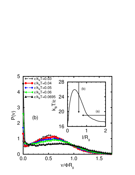
Figure 8: Subbox analysis of the local $A$-monomer density distribution:
(a) Dependence on the layer thickness above the wetting transition ($\epsilon/k_{B}T=0.0695$). Upon reducing the layer thickness the distribution becomes bimodal; this indicates prewetting. The distribution of a thin film above the prewetting critical point ($\epsilon/k_{B}T=0.03$) is also shown for comparison.
(b) Temperature dependence of the local lateral A-monomer density. At high temperature the distribution is nearly Gaussian; whereas it becomes bimodal at low temperatures but above the wetting transition.
The inset illustrates the different path to coexistence in (a) and (b). The solid curve, depicting the thickness of the coexisting layers, is obtained from the SCF calculations.

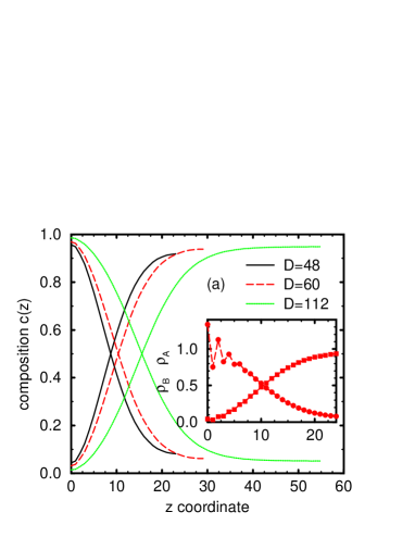
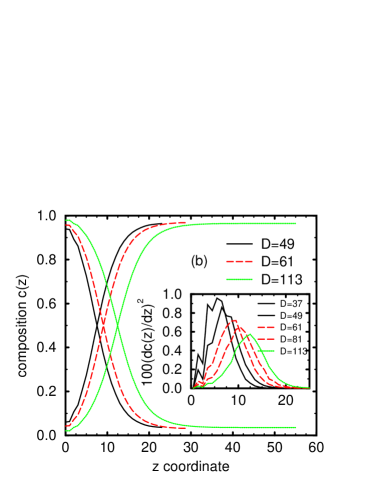
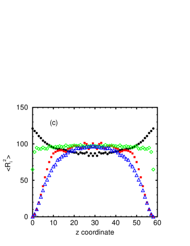
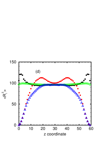
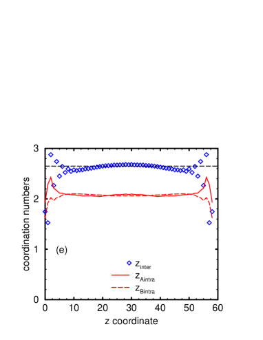
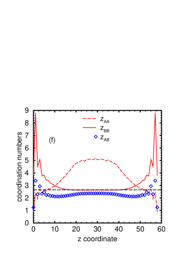
Figure 9: Profiles across the film:
(a) Monte Carlo results for the composition profiles $c(z)=\rho_{A}(z)/(\rho_{A}(z)+\rho_{B}(z))$ at $\epsilon/k_{B}T=0.02$, $\epsilon_{\rm w}/k_{B}T=0.16$ and thickness $D$ as indicated in the figure. The inset shows the A- and B-monomer densities near the wall for $D=60$.
(b) Composition profiles at the interaction as in (a) calculated in the self-consistent field theory. The inset displays the squared composition gradient.
(c) Chain extension for $D=60$ as function of the distance from the wall. Filled circles represent $\langle R_{\|}^{2}\rangle$ of A-chains, filled squares denote $\langle R_{\perp}^{2}\rangle$ of A-chains, and diamonds, triangles correspond to $\langle R_{\|}^{2}\rangle$, $\langle R_{\perp}^{2}\rangle$ of B-chains respectively.
(d) Chain extensions for $D=61$ in the mean field calculations. Symbols are the same as in (c).
(e) MC results for the total number of intermolecular contacts and intrachain contacts as a function of the distance from the wall ($D=60$)
(f) Intermolecular contacts between like and unlike monomer species as a function of the distance from the wall ($D=60$) in the MC simulations. Rather pronounced non-random mixing effects are observed.

Figure 10: Kelvin equation and thickness of the wetting layer:
(a) MC (circles) and SCF (squares) results for the coexistence chemical potential difference $\Delta\mu$ at $\epsilon=0.02$, $\epsilon_{\rm w}=0.16$. The solid lines correspond to eq. (5), where the slope is fixed by the independently measured interfacial tension.
(b) Thickness $l$ of the wetting layer in the MC simulations (circles) and SCF calculations (squares). The slope is a measure for the wall-interface interaction range $1/\lambda$.

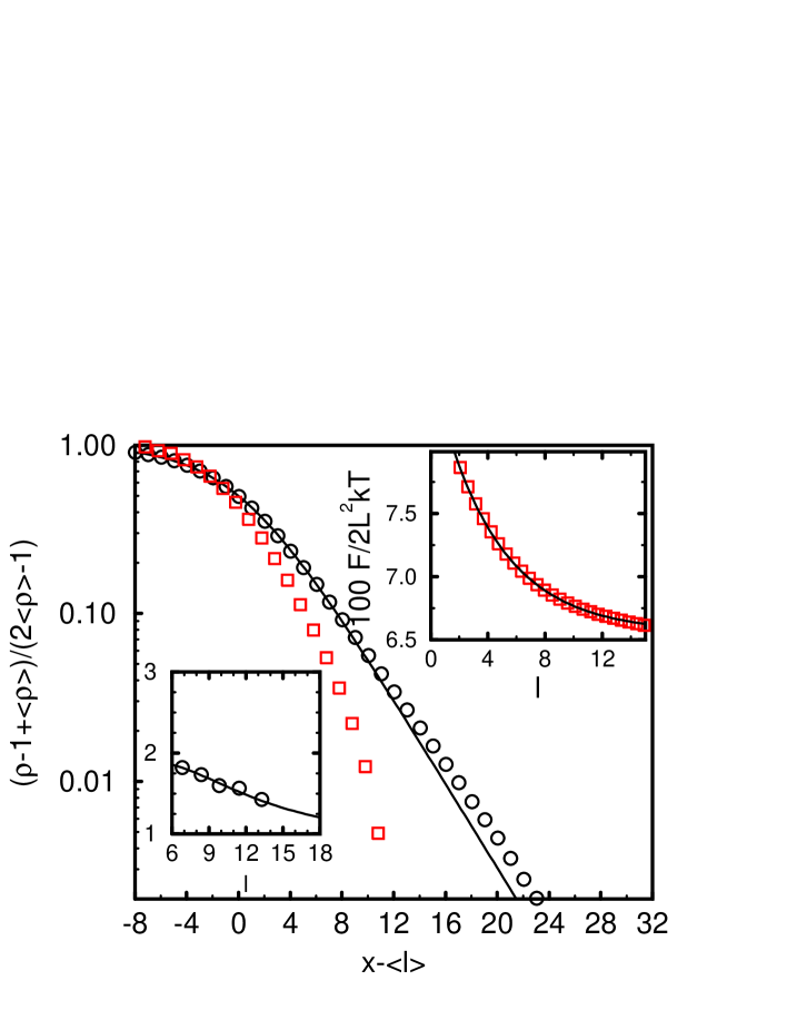
Figure 11: Interfacial profiles in the self-consistent field calculation: Circles denote the interfacial profile in the bulk ($64\times 64\times 128$ geometry and periodic boundary conditions), and the solid line presents a tanh-profile with width $w=6.91$. There are deviations in the wings of the profile. Squares represent the profile in the confined system $D=49$.
The right inset presents the effective interface-wall potential in the self-consistent field calculations for $D=49$, $\epsilon/k_{B}T=0.02$ and $\epsilon_{\rm w}/k_{B}T=0.16$. The solid line is a fit with an exponential decaying interaction $g(l)=0.0656+0.0209\exp(-0.231l)$. (This corresponds to a parallel correlation length of $\xi_{\|}(\sigma_{AB}/\sigma)^{1/2}\approx 43$)
The left inset displays the position dependence of the effective interfacial tension $\Sigma$. The solid line corresponds to $\Sigma/\Sigma_{AB}=1+2.4(0.21l)\exp(-0.21l)$

References

- [1] Cahn J. W. J.Chem.Phys. 1977, 66 , 3667.
- [2] Binder K. Adv.Poly.Sci. in press. Binder K. Acta Polymer 1995, 46, 204.
- [3] Binder K.; Landau D. P. Phys.Rev. 1988, B 37, 1745. Binder K.; Landau D. P. J.Chem.Phys. 1992, 96, 1444. Binder K.; Ferrenberg A. M.; Landau D. P. Ber.Bunsenges.Phys.Chem. 1994, 98 340.
- [4] Schick M., Les Houches lectures on “Liquids at interfaces” 1990, Elsevier Science Publishers B.V. Dietrich S., in Phase Transitions and Critical Phenomena, Vol. 12, C. Domb and J.L. Lebowitz (eds), NY Academic Press 1988.
- [5] Forgacs G.; Lipowsky R.; Nieuvenhuizen T. in Phase Transitions and Critical Phenomena, Vol. 14, Domb C.; Lebowitz J. L. (eds) NY Academic Press.
- [6] Parry A. O. J.Phys.Cond.Matt. 1996, 8, 10761. Evans R. J.Phys.Cond.Matt. 1990, 2, 8989. Evans R.; Marini U.; Marconi B.; Tarazona P. J.Chem.Phys. 1986, 84, 2376.
- [7] de Gennes P. G. Rev.Mod.Phys 1985, 57, 827.
- [8] Young T. Philos.Trans.R.Soc.London 1805, 5, 65.
- [9] Qu S.; Clarke J.; Liu Y.; Rafailovich M. H.; Sokolov J.; Phelan K. C.; Krausch G. Macromolecules 1997, 30, 3640.
- [10] Schmidt I.; Binder K. J.Phys. 1985, 46, 1631.
- [11] Fisher M. E.; Nakanishi H. J.Chem.Phys. 1981, 75, 5857. Nakanishi H.; Fisher M. E. J.Chem.Phys. 1983, 78, 3279.
- [12] Parry A. O.; Evans R. J.Phys.A 1992, 25, 275.
- [13] Nakanishi H.; Pincus P. J.Chem.Phys. 1983, 79, 997.
- [14] Carmesin I.; Noolandi J. Macromolecules 1989, 22, 1689).
- [15] Flebbe T.; Dünweg B.; Binder K. J.Phys.II. 1996, 6, 667.
- [16] Jones R. A. L. Polymer 1994, 35, 2161.
- [17] Scheffold F.; Eiser E.; Budkowski A.; Steiner U.; Klein J.; Fetters L. J. J.Chem.Phys. 1996, 104, 8786 and 8795.
- [18] Budkowski A.; Scheffold F.; Klein J.; Fetters L. J. J.Chem.Phys. 1997, 106, 719.
- [19] Hariharan A.; Kumar S. K.; Rafailovich M. H.; Sokolov J.; Zheng X.; Duong D.; Schwarz S. A.; Russell T. P. J.Chem.Phys. 1993, 99, 653.
- [20] Genzer J.; Faldi A.; Oslanec R.; Composto R. J. Macromolecules 1996, 29, 5438.
- [21] Zhao W.; Rafailovich M. H.; Sokolov J.; Fetters L. J.; Plano R.; Sanyal M. K.; Sinha S. K. Phys.Rev.Lett 1993, 70, 1453.
- [22] Wang J. S.; Binder K. J.Chem.Phys. 1991, 94, 8537, Pereira G. G.; Wang J. S. J.Chem.Phys. 1996, 105, 3849. Pereira G. G.; Wang J. S. J.Chem.Phys. 1996, 104, 5294. Pereira G. G.; Wang J. S. Phys Rev 1996, E 54, 3040 . Pereira G. G.; Wang J. S. J.Chem.Phys. 1997, 106, 4282. Pereira G. G. J.Chem.Phys. 1997, 107, 3740.
- [23] Kumar S. K.; Tang H.; Szleifer I. Mol.Phys. 1994, 81, 867.
- [24] Rouault Y.; Dünweg B.; Baschnagel J.; Binder K. Polymer 1996, 37, 297.
- [25] Noolandi J.; Hong K. M. Macromolecules 1981, 14, 727, ibid 1982, 15, 483.
- [26] Genzer J.; Composto R. J. J.Chem.Phys. 1997, 106, 1257, Genzer J.; Faldi A.; Composto R. J. Phys.Rev. 1996, E 50, 2372. Genzer J.; Composto R. J. Euro.Phys.Lett. 1997, 38, 171.
- [27] Schmid F. J.Chem.Phys. 1996, 104, 9191.
- [28] Nath S. K.; McCoy J. D.; Donley J. P.; Curro J. G. J.Chem.Phys. 1995, 103, 1635.
- [29] Freed K. F. J.Chem.Phys. 1996, 105, 10572.
- [30] Cohen S. M.; Muthukumar M. J.Chem.Phys. 1989, 90, 5749.
- [31] Jerry R. A.; Nauman E. B. J.Chem.Phys. 1992, 97, 7829.
- [32] Rouault Y.; Baschnagel J.; Binder K. J.Stat.Phys. 1995, 80, 1009.
- [33] Tang H.; Szleifer I.; Kumar S. K. J.Chem.Phys. 1994, 100, 5367.
- [34] Müller M.; Werner A. J.Chem.Phys. 1997, 107, 10764.
- [35] Müller M.; Schick M. J.Chem.Phys. 1996, 105, 8885, Müller M.; Schick M. J.Chem.Phys. 1996, 105, 8282.
- [36] Szleifer I.; Ben-Shaul A.; Gelbhart W. M. J.Chem.Phys. 1986, 85, 5345, ibid. 1987, 86, 7094.
- [37] Müller M.; Schick M., Macromolecules 1996, 29, 8900.
- [38] There are corrections to the coefficient of the next to leading term , due to the shift of the chemical potential and corrections to the interfacial tension.
- [39] Bitsanis I.; Hadziioannou G.;, J.Chem.Phys 1990, 92, 3827.
- [40] Binder K.; Frisch H. L. Macromolecules 1984, 17, 2928.
- [41] Werner A.; Schmid F.; Müller M.; Binder K. J.Chem.Phys. 1997, 107, 8175 .
- [42] Helfrich W. Z.Naturforsch. 1973, 28c, 693. Canham P. B. J.Teor.Biol. 1970, 26, 61. Evans E. Biophys.J. 1974, 14, 923.
- [43] Parry A. O.; Boulter J. C. Physica 1995, A 218, 77, ibid 109.
- [44] The restriction of interfacial fluctuations due to the presence of the wall gives rise to an additional repulsion, which, decays Gaussian[4], however.
- [45] Carmesin I.; Kremer K. Macromolecules 1988, 21, 2819. Deutsch H.-P.; Binder K. J.Chem.Phys. 1991, 94, 2294.
- [46] Müller M.; Binder K. Macromolecules 1995, 28, 1825.
- [47] Müller M.; Binder K.; Oed W. Faraday Trans. 1995, 91, 2369.
- [48] Müller M.; Wilding N. B. Phys.Rev. 1995, E 51, 2079.
- [49] Schmid F.; Müller M. Macromolecules 1995, 28, 8639.
- [50] Sariban A.; Binder K. Macromolecules 1988, 21, 711.
- [51] Rouault Y.; Baschnagel J. private communication.
- [52] Torrie G. M.; Valleau J. P. Chem.Phys.Lett. 1974, 28, 578.
- [53] Berg B. A.; Neuhaus T. Phys.Rev.Lett. 1992, 68, 9.
- [54] Ferrenberg A. M.; Swendsen R. H. Phys.Rev.Lett. 1988, 61, 2635, ibid 1989, 63, 1195. Bennett A. J.Comp.Phys. 1979, 22, 245.
- [55] Helfand E.; Tagami Y. J.Polym.Sci.,Polym.Lett. 1971, 9, 741. Helfand E.; Tagami Y. J.Chem.Phys. 1972, 56, 3592. Helfand E. J.Chem.Phys 1975, 62, 999.
- [56] Shull K. R. Macromolecules 1993, 26, 2346.
- [57] Scheutjens J. M. H. M.; Fleer G. J. J.Phys.Chem. 1979, 83 ,1619, ibid 84 , 178.
- [58] Scheutjens J. M. H. M.; Fleer G. J. Macromolecules 1985, 18, 1882.
- [59] Szleifer I. in “Current Opinion in Colloid and Interface Science” 1997, 1, 416.
- [60] Szleifer I.; Carignano M. A. Adv.Chem.Phys. 1996, 94, 742.
- [61] Due to the extended shape of the monomers in the bond fluctuation model the front, lower, left corner of a monomer cannot occupy the lattice layer .
- [62] The compressibility of the athermal system has been measured in Müller M.; Paul W. J.Chem.Phys. 1994, 100, 719. , where denotes the entropy density.
- [63] Weinhold J. D.; Kumar S. K.; Szleifer I. Europhys.Lett. 1996, 35, 695.
- [64] The coordination number z, as determined via the intermolecular pair correlation function[47] is slightly temperature dependent:
- [65] Matsen M. W.; Schick M. Phys.Rev.Lett. 1994, 72, 2660.
- [66] Matsen M. W. J.Chem.Phys. 1997, 106, 7781.
- [67] Schlangen L.; Leermakers F. A. M.; Koopal L. K., Faraday Trans 1996, 92, 579.
- [68] Binder K. Phys.Rev. 1992, A 25, 1699.
- [69] Borgs C.; Kotecky K. J.Stat.Phys. 1990, 61, 79, Phys.Rev.Lett. 1992, 68, 1734.
- [70] Binder K. Phys.Rev.Lett. 1981, 47, 693.
- [71] Wilding N. B. Phys.Rev. 1995, E 52, 602. Wilding N. B. J.Cond.Matter 1997, 9, 585.
- [72] Kamienarz G.; Bloete H. W. J. J.Phys. 1993, A 26, 201.
- [73] Peterson B. K.; Gubbins K. E.; Heffelfinger G. S.; Marini U.; Marconi B.; van Swol F. J.Chem.Phys. 1988, 86, 6487.
- [74] Semenov A. N. J.de.Phys. 1996, II 6, 1759.
- [75] Cifra P.; Bruder F.; Brenn R.;, J.Chem.Phys. 1993, 99, 4121.
- [76] Indeed, the prewetting line in the semi-infinite system approaches the coexistence curve for very closely. However, due to the small wall separation , the two interfaces interact with each other across the film. This interaction across the film modifies the dependence of the free energy on the layer thickness such that only a single layer thickness is stable on the A-poor side of the phase diagram.
- [77] Aubouy M.; Phys.Rev. 1997, E 56, 3370.
- [78] Brochard F.; Daillant J. Can.J.Phys. 1990, 68, 1084.
- [79] Binder K. in Material Science and Technology, Vol. 5, Phase Transformation in Materials, p.405, Haasen P.(ed), VCH Weinheim 1991.
-
[80]
mpeg movies of the time evolution are available under
http:
www.cond-mat.physik.uni-mainz.de/~ mueller - [81] Szleifer I.; Carignano M. A. Europhys.Lett. 1995, 30, 525.
- [82] Binder K.; Evans R.;, Landau D. P.; Ferrenberg A. M. Phys.Rev. 1996, E 53, 5029.
- [83] Ginzburg V. L. Sov.Phys.Solid State 1960, 2, 1824. de Gennes P. G. J.Phys.Lett. (Paris) 1977, 38, L-441. Binder K. Phys.Rev. 1984, A 29, 341.
- [84] Jin A. J.; Fisher M. E. Phys.Rev. 1993, B 47, 7365.
- [85] Berg B. A.; Hansmann U.; Neuhaus T. Z.Phys. 1993, B 90, 229.
- [86] For a typical potential at the wetting transition the system always chooses the asymmetric state and .