Magneto-optical study of magnetic flux penetration into a current-carrying high-temperature superconductor strip

Abstract

Magnetic flux distribution across a high-temperature superconductor strip is measured using magneto-optical imaging at 15 K. Both the current-carrying state and the remanent state after transport current are studied up to the currents $0.97I_{c}$ where $I_{c}$ is the critical current. To avoid overheating of the sample current pulses with duration 50 ms were employed. The results are compared with predictions of the Bean model for the thin strip geometry. In the current-carrying state, reasonable agreement is found. However, there is a systematic deviation – the flux penetration is deeper than theoretically predicted. A much better agreement is achieved by accounting for flux creep as shown by our computer simulations. In the remanent state, the Bean model fails to explain the experimental results. The results for the currents $I\leq 0.7I_{c}$ can be understood within the framework of our flux creep simulations. However, after the currents $I>0.7I_{c}$ the total flux trapped in a strip is substantially less than predicted by the simulations. Furthermore, it decreases with increasing current. Excessive dissipation of power in the annihilation zone formed in the remanent state is believed to be the source of this unexpected behavior.

I Introduction

Spatially resolved studies of magnetic flux penetration into high-temperature superconductor (HTSC) films are extensively performed during the last few years. Modern experimental techniques, in particular Hall micro-probe measurements and magneto-optical (MO) techniques, allow local magnetic field distributions in various HTSC structures to be investigated with rather high spatial resolution. As a result, a quantitative comparison between experimental flux density profiles and theoretical predictions has become possible. Most of the comparisons are done within the framework of the critical state model (CSM)[1]. Based on this model theoretical calculations of the field distributions for many practical geometries are carried out. In particular, the flux profiles in an infinite thin strip placed in a perpendicular magnetic field, or carrying a transport current are calculated in Refs. [2, 3, 4]. Most experimental studies of flux penetration, see e. g. Refs. [5, 6, 7, 8], are focused on the behavior of samples placed in an external magnetic field, as well as on the remanent state after the field is switched-off. The results appear in a good agreement with experiment.

Meanwhile, we are aware of only a few papers devoted to experimental investigation of the self-field of transport currents [9, 10, 11, 12, 13, 14, 15, 16]. Unfortunately, these investigations do not allow a simple comparison to the theory. Indeed, some of them[9, 12, 13, 14, 15, 16] present results for samples of rather complicated geometry, e. g., for tapes. Others[10, 11] report results for currents much less than the critical current, $I_{c}$.

The aim of this work is to study by MO imaging the flux penetration into a strip with transport current. It seems most interesting to have the current $I$ as close as possible to the critical one. To reach this aim one needs narrow strips where the critical current is not too large to be carried by contacts without their destruction. On the other hand, the wider the strip the better the relative spatial resolution of MO imaging. By optimizing both the strip’s width and other experimental conditions we managed to obtain flux profiles both in the current-carrying and in the remanent state with a resolution sufficient for comparison with theory.

In Sec. II the samples and the experimental technique are described. The results for flux profiles and reconstructed current distributions are compared to the CSM in Sec. III. It is shown that the deviations are fairly small in the current-carrying state. However, they are pronounced in the remanent state after applied current. The main deviation is a deeper flux penetration inside the strip compared to predictions of the CSM. To understand the source of the deviation we have carried out numerical simulations of the field and current profiles taking into account flux creep. The results of these simulations are discussed in Sec. IV. Creep appears to explain all the experimental results for the current-carrying state, as well as the results for the remanent state after relatively small currents, $I\lesssim 0.7\,I_{c}$. In the remanent state after large currents the experimental profiles could not be explained either by CSM or by flux creep. It seems that thermal effects are responsible for this behavior.

II Experimental

A Sample preparation

Films of YBa₂Cu₃O_7-δ were grown by dc magnetron sputtering [17] on LaAlO₃ substrates. X-ray and Raman spectroscopy analysis confirmed that the films were $c$-axis oriented and of a high structural perfection. Several bridges were formed from each film by a standard lithography procedure. Their dimensions are $500\times 110\times 0.2$ $\mu$m³. To minimize temperature increase caused by Joule heating the contact pads were made as wide as possible. They are displaced to the side of the structure allowing the MO indicator film to be placed as close to the bridge as possible. To provide low contact resistance they were covered with a Ag layer, and Au wires of 50 $\mu$m diameter were attached by thermal compression. The boundary resistance of Ag/YBa₂Cu₃O_7-δ interface was as low as 10${}^{-3}-10^{-4}\,\Omega\,$cm², while the area of one contact pad was $\approx 0.25$ cm². The bottom of 500 micron substrate was held at a constant temperature. Since the thermal conductivity of LaAlO₃ is[18] 0.1 W/(cm   K), the temperature rise at the interface induced by Joule heating due to currents up to 6 A is always less than 0.1 K. Thus, resulting heating of the YBa₂Cu₃O_7-δ bridge situated 500 micron away from the contact pads is negligible.

An initial selection of the structures having the smoothest surface, i.e., height of over-growth less than 3 $\mu$m, was made using SEM. Next, bridges with pronounced weak links, $T_{c}$-inhomogeneities and other defects which reduce the total critical current $I_{c}$ were eliminated by means of low-temperature SEM,[19] in addition to current-voltage measurements made by a standard four-probe scheme. As a result, the bridges used for the final investigations had a critical current density, $j_{c}$, larger than $10^{6}$ A/cm² at 77 K.

B Magneto-optical imaging

Our flux visualization system is based on the Faraday rotation of a polarized light beam illuminating an MO-active indicator film that we place directly on top of the sample’s surface. The rotation angle increases with the magnitude of the local magnetic field perpendicular to the HTSC film. By using crossed polarizers in an optical microscope one can directly visualize and quantify the field distribution across the sample area. As Faraday-active indicator we use a Bi-doped yttrium iron garnet film with in-plane anisotropy[20]. The indicator film was deposited to a thickness of 5 $\mu$m by liquid phase epitaxy on a gadolinium gallium garnet substrate. Finally, a thin layer of aluminum was evaporated onto the film in order to reflect the incident light and thus providing a double Faraday rotation of the light beam. The images were recorded with an eight-bit Kodak DCS 420 CCD camera and transferred to a computer for processing. The conversion the gray level of the image into magnetic field values is based on a careful calibration of Bi:YIG indicator response to a range of controlled perpendicular magnetic field as seen by the CCD camera through the microscope (see also Ref. [5]). After each series of measurement, the temperature was increased above $T_{c}$ and the in-situ calibration of the indicator film was carried out. As a result, possible errors caused by inhomogeneities of both indicator film and light intensity were excluded.

To avoid overheating of the HTSC bridges as the current approaches $I_{c}$ a specific experimental procedure was developed. Short current pulses were applied and synchronized with the camera recording as shown in Fig. 1.

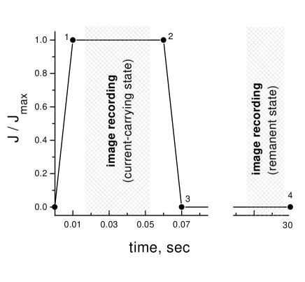
FIG. 1.: Temporal profile of the pulsed transport current. The exact time intervals of the MO image recording in the current-carrying state and the subsequent remanent state are indicated.

The transport current with a rise time of 10 ms was applied 20-30 ms before an image was recorded. The exposure time was 35 ms, after which the current was ramped to zero in 10 ms. After waiting another 20-30 seconds the remanent field distribution was measured.

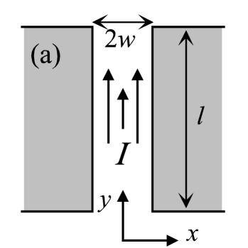
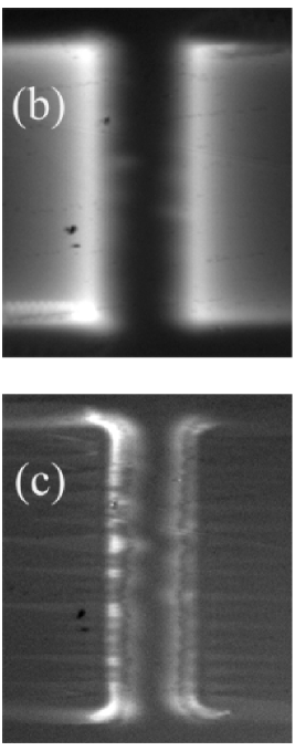
FIG. 2.: (a) Sketch of the studied YBa₂Cu₃O_7-δ bridge structure. (b) MO image of flux distribution with the bridge in the current-carrying state with $I=4.16$ A. (c) MO image of flux distribution with the bridge in the remanent state after the applied-current state shown in (b). Two inner bright lines near the sample edges represent the original trapped flux, the outer bright lines represent penetration of the oppositely directed return field, while dark lines between them correspond to regions of vortex-antivortex annihilation. Strong contrast enhancement was applied to the image in (c).

III Results and comparison with CSM

Throughout the paper we use the following notations, see Fig. 2. The $x$-axis is directed across the bridge, the edges being located at $x=\pm w$. The $y$-axis points along the bridge, and the $z$-axis is normal to the film plane. The $z$-component of the flux density is denoted by $B$. The profiles $|B(x)|$ were always measured for a fixed $y$ in the central part of the strip minimizing the effect of the stray field of the contact pads. Although the MO measurements give the distribution of $|B(x)|$, we could in the simple geometry under consideration always determine the sign of $B$ by inspection of the images. We let $J(x)$ denote the sheet current density defined as $J(x)=\int{j(x,z)dz}$, where $j(x,z)$ is the current density. For brevity, we will often use current density also for $J(x)$. As the bridge thickness is much less than its width, the theoretical results for the thin strip geometry[3, 4] are used below. In our experiments, the bridge thickness is also of the order of the penetration depth $\lambda$, hence its magnetic properties are fully characterized by the two-dimensional flux distribution at the surface.

A Current-carrying bridge

Flux density distributions for a strip carrying a transport current $I$ were measured for currents up to $I$=5.72 A. The MO image for the current $I=4.16$ A is shown in Fig. 2(b). Three profiles of the flux density $|B(x)|$ taken across the strip are shown in Fig. 3. The profiles have maxima near the strip edges and a minimum in between. Actually, the left and the right parts of the profiles correspond to induction of opposite sign. As the current increases, (a)-(c), the magnetic flux penetrates deeper and the flux free Meissner region in the center of the bridge decreases in size.

The experimental MO data are interpreted in the framework of the CSM. As discussed in Ref. [5], one should account for the finite distance between the sample and the MO indicator film. The perpendicular magnetic field, $B$, at the height $h$ above the center of the bridge can be calculated from the current density distribution $J(x)$ as[5]

$$B(x)=\frac{\mu_{0}}{2\pi}\int_{-w}^{w}{\frac{x^{\prime}-x}{h^{2}+\left(x^{\prime}-x\right)^{2}}\,J(x^{\prime})\,dx^{\prime}\,+B_{a}.}$$ (1)

Here $B_{a}$ is the external magnetic induction. The current density distribution in a strip carrying a transport current $I$ can be written for the Bean model as[3, 4]

$${\frac{J(x)}{J_{c}}}=\left\{\begin{array}[]{lr}\displaystyle{\frac{2}{\pi}}\arctan\left(\sqrt{\displaystyle{\frac{w^{2}-a^{2}}{a^{2}-x^{2}}}}\right),&|x|<a\\ 1,&a<|x|<w\end{array}\right.,$$ (2)

where $a=w\sqrt{1-(I/I_{c})^{2}}$, and $I_{c}=2w\,J_{c}$ is the critical current. As Eqs. (1) and (2) yield a symmetric $|B(x)|$-profile we find it necessary to account also for the stray field of the contact pads in order to reproduce the slight asymmetry in the $|B(x)|$ data. The current in the pads produces near the central part of the bridge a magnetic field which acts as an additional external field varying slowly in space. This allows us to employ the results of the CSM for the case of a transport current superimposed by a weak external magnetic field.[21] According to this theory[3, 4], the current density distribution Eq. (2) is modified to yield $J(x)=J_{c}$ at $x$ within the intervals $(-w,p-a)$, $(p+a,w)$ and

$$\displaystyle{\frac{J(x)}{J_{c}}} = \displaystyle{\frac{1}{\pi}}\left(\arcsin\displaystyle{\frac{(x-p)(w-p)-a^{2}}{a(w-x)}}\right.$$ (4)

$$\left.-\arcsin\displaystyle{\frac{(x-p)(w+p)+a^{2}}{a(w+x)}}\right)+1$$

for $p-a<x<p+a$. Here

$$a = \frac{w}{\cosh\left(B_{a}/B_{c}\right)}\sqrt{1-\left(\frac{I}{I_{c}}\right)^{2}},$$

$$p =w \frac{I}{I_{c}}\tanh\left(\frac{B_{a}}{B_{c}}\right)\,,\quad B_{c}\equiv\frac{\mu_{0}J_{c}}{\pi}\,.$$

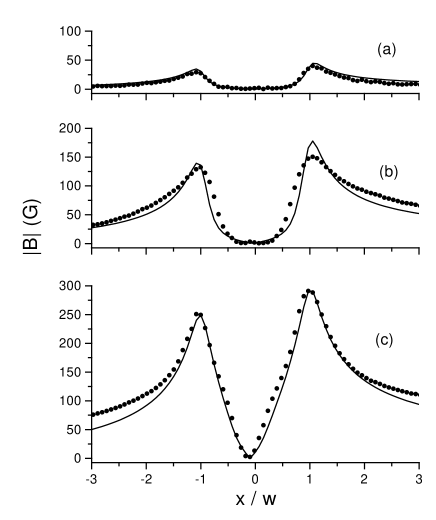
FIG. 3.: Profiles of the perpendicular magnetic field produced at a distance $h=8\ \mu$m above the bridge carrying transport currents. Symbols show the experimental data (only 1/5 of all measured points are shown), and the solid lines represent CSM calculations from the Eqs.(4) and (1). $I/I_{c}=0.13$(a), 0.53(b), 0.97(c), where $I_{c}=5.9$ A.

Profiles of $|B(x)|$ calculated from Eqs. (4) and (1) are shown in Fig. 3 by the solid lines. Here $I_{c}$ and $h$ are parameters determined by fitting the CSM profiles to experimental data. The values $I_{c}=5.9$ A, $h=8\ \mu$m yield the best fit for the profiles measured at all currents $I$. Note that $I_{c}$ has a physical meaning of the critical current for CSM model, at which the magnetic field fully penetrates the bridge.

One can notice in such experiments, and e. g. in Fig. 3(b), that the experimental penetration of the magnetic field is deeper than the CSM prediction. This characteristic deviation can be accounted for by introducing flux creep, as will be discussed in detail in the next section.

With $h$ being a known parameter one can also directly determine the current distributions across the strip, $J(x)$, from the experimental $B(x)$-profiles. This can be done on a model-independent basis according to an inversion scheme developed in Ref. [5]. Since the accuracy of the inversion is limited by the distance $h$, we chose a step size along the $x$-axis close to $\Delta=h/2$. Specifying the coordinates in units of $\Delta$, i.e., $x=n\Delta,\ x^{\prime}=n^{\prime}\Delta,\ h=d\Delta$, and applying a Hannig window filtering function one obtains[5]:

$$J(n)=\sum_{n^{\prime}}\frac{n-n^{\prime}}{\mu_{0}\pi}\left(\frac{1-(-1)^{n-n^{\prime}}e^{\pi d}}{d^{2}+(n-n^{\prime})^{2}}\right.$$ (5)

$$\left.\ +\frac{\left[d^{2}+(n-n^{\prime})^{2}-1\right]\left[1-(-1)^{n-n^{\prime}}e^{\pi d}\right]}{\left[d^{2}+(n-n^{\prime}+1)^{2}\right]\left[d^{2}+(n-n^{\prime}-1)^{2}\right]}\right)B(n^{\prime}).$$ (6)

The current density profiles calculated from experimental $B(n)$-data using this formula are shown in Fig. 4. The figure also shows the results obtained from Eq. (4) using the value of $I_{c}$ determined by the fitting of $|B(x)|$-profiles. As seen from Fig. 4, the experimental profiles trace all qualitative features of the theoretical curves. In particular, the minimum in the current density near the bridge center predicted by the CSM can clearly be distinguished in all experimental curves. Moreover, the position of the minimum is found to be slightly shifted towards negative $x$, a behavior in full agreement with the theory when the effect of contact pad stray fields is accounted for.

As first pointed out in Ref. [5], the MO YIG indicators with in-plane anisotropy respond not only to $B_{z}$ but also to the component $B_{x}$ parallel to the film. In the data presented we always made the proper corrections according to the method suggested in Ref. [5], i.e., $B_{x}(x)$ component was calculated from the current profiles by Biot-Savart law and then used to re-normalize the profile $B_{z}(x)$. This procedure is converging very rapidly.

To check self-consistency of our inversion calculations we integrated the current density over $x$. Indeed, The total current was always equal to the transport current passed through the bridge within an accuracy of $5\%$.

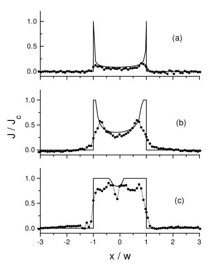
FIG. 4.: Distributions of current density in the current-carrying strip. Symbols show the distributions inferred from experimental data using Eq. (6). The predictions of the CSM, Eq. (4) are shown as full lines. $I/I_{c}=0.13$(a), 0.53(b), 0.97(c), where $I_{c}=5.9$ A.

Some deviations between experimental and theoretical current profile slopes are seen near the sample edges where the theoretical profiles are discontinuous. The observed smearing of the current profiles reconstructed from the induction data can be ascribed mainly to discreteness of the points used in the inverse calculation, and possibly a slight structural imperfections near the very edge of the sample.

B Bridge in a remanent state after transport current

When the transport current $I$ is switched-off, the magnetic flux in the inner part of the strip remains trapped. The return field of this trapped flux will re-magnetize the edge regions of the strip and the flux of opposite sign penetrates an outer rim. As a result, the measured remanent distribution $|B(x)|$ should display two peaks in each half of the bridge; one representing the maximum trapped flux, and another near the edge indicating the maxima in the reverse flux. In this oscillatory flux profile typical values of $|B_{z}|$ are significantly lower than in the current-carrying state. Thus, MO studies become substantially more difficult in the remanent state, and flux profiles with reasonable signal-to-noise ratio were recorded only after relatively large transport currents, $I>0.6I_{c}=3.68$ A.

The MO image of flux density distribution in the remanent state after switching off a transport current of 4.16 A is shown in Fig. 2(c). Figure 5 shows the flux density profile taken across the strip in this remanent state. It can be seen that there are large maxima of trapped flux in the center of the bridge. Also, the weaker maxima of reverse flux are visible near the edges. In the figure we have removed the experimental points corresponding to the regions where the MO image is governed by disturbing zig-zag domain pattern in the indicator film. This occurs where $B_{x}$ changes sign.

The current distribution derived from the Bean model for the remanent state is[3, 4]

$${\frac{J(x)}{J_{c}}}=\left\{\begin{array}[]{lc}\displaystyle{\frac{2}{\pi}}\left[\arctan\left(\sqrt{\displaystyle{\frac{w^{2}-a^{2}}{a^{2}-x^{2}}}}\right)-2\arctan\left(\sqrt{\displaystyle{\frac{w^{2}-b^{2}}{b^{2}-x^{2}}}}\right)\right],&-a<x<a,\\ 1-\displaystyle{\frac{4}{\pi}}\arctan\left(\sqrt{\displaystyle{\frac{w^{2}-b^{2}}{b^{2}-x^{2}}}}\right),&a<|x|<b\end{array}\right.\,,$$ (7)

where $a=w\sqrt{1-(I/I_{c})^{2}},\ b=w\sqrt{1-(I/2I_{c})^{2}}$ and $I$ is the maximal current. At $b<|x|<w$ the current density is equal to $-J_{c}$. The small contribution from the field generated by the contact remanent currents is here neglected.

The magnetic field profiles calculated using Eqs. (7) and (1) are shown in Fig. 5 (solid line) together with the experimental data. We used the same values for $I_{c}$ and $h$ as obtained by fitting results for current-carrying state. Evidently, there is here a significant deviation between our data and the CSM description. The main deviation is that the trapped flux maxima in the experimental curve are shifted towards the center. Again, this can be shown to be an effect of flux creep as discussed in the next section. Another deviation seen in Fig. 5 is that the maxima near the edges are hardly visible experimentally. This is most likely due to the nonlinear response of the optical detection system which leads to reduced sensitivity at low Faraday rotation angles, i.e., at small induction values. Another source of smearing is that the width of the maxima near the edges is comparable to the thickness of MO indicator film.

The experimental flux profiles in the remanent state after large currents $I>4.16$ show even more intriguing behavior. Fig. 6 shows six remanent flux profiles across the right half of the bridge after applying currents ranging from 4.42 A to 5.72 A. The observed decrease of the trapped flux with increasing transport current seems highly unexpected. Such a behavior definitely contradicts the CSM. To make a quantitative comparison we have integrated the flux trapped in the band $-0.4w<x<0.2w$ , where the MO data are reliable. The dependence of the total flux on the current is shown in Fig. 7. At small currents, $I\leq 4.16$ A, the behavior is normal as the amount of trapped flux increases with the current. At larger currents, however, the trapped flux levels out and even starts to decrease as $I$ approaches $I_{c}$. The full line in the same figure indicates the predictions of the CSM, which clearly shows a different behavior. Neither is the non-monotonous behavior seen experimentally explained by flux creep.

Let us sum up the comparison with the CSM for the current-carrying and remanent states. The general features of flux distribution in a strip with transport current predicted by the CSM are well confirmed by the experiments. It should be noted that such a good agreement was achieved only by taking into account a finite distance between the HTSC film and the MO indicator, the

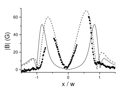
FIG. 5.: Remanent profiles of the absolute value of perpendicular magnetic field at the distance $h=8\ \mu$m above the bridge after applying transport current $I=4.16$ A. Dots – experiment, solid line – CSM, Eqs. (7), (1) with $I_{c}=5.9$ A, dashed line – flux creep simulations. A large amount of flux trapped near the bridge center is in strong contradiction with CSM and can be explained by flux creep. Experimental points in the regions where the parallel component $B_{x}(x)$ changes sign and the response of indicator film is suppressed have been removed from the plot.

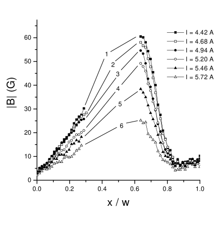
FIG. 6.: Experimental profiles of the absolute value of perpendicular magnetic field in the remanent state after different transport currents $I$: (1) - 4.42 A, (2) - 4.68 A, (3) - 4.94 A, (4) - 5.20 A, (5) - 5.46 A, (6) - 5.72 A. Only the right half of the bridge is shown. Note the unusual $I$-dependence of the trapped flux: the larger the current the smaller the density of trapped flux in the bridge.

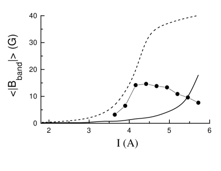
FIG. 7.: Flux trapped within the band $\,-0.4w<x<0.2w\,$ in the remanent state after transport current $I$ as a function of $I$. The band corresponds to reliable MO data shown in Fig. 5, the flux in normalized to the band width. Dots – experimental results. Solid and dashed lines – CSM and flux creep simulations respectively. For $I\leq 4.16$ A the experiment is in a qualitative agreement with flux creep, however for larger currents a striking steady decrease in trapped flux is observed.

additional field generated by contact currents, and the influence of parallel field component on the properties of YIG indicator. However, a general trend of a deeper flux penetration compared to the CSM prediction can be traced. In the remanent state the deviations from the CSM are more pronounced, and experimental flux profiles after currents $I>0.7I_{c}$ have qualitatively different shape. In particular, the flux trapped inside the bridge can be several times greater than predicted and it depends on the previously applied current in a non-monotonous way.

Comparing the experimental results with the predictions of CSM we employed the expressions (4) and (7) based on the Bean model. Thus, we assumed the critical current density $J_{c}$ to be $B$-independent. We have checked validity of this assumption studying penetration of an applied magnetic field into a bridge of the same geometry fabricated on the same film. We could trace rather weak dependence of $J_{c}$ versus $B$ only above $B\approx 200$ G. For smaller $B$ all the results, including the results for the remanent state after external field, were compatible with the CSM predictions, as in Ref. [5]. Consequently, there is no reason to attribute the deviations observed in the transport current regime to a $B$-dependence of $J_{c}$.

IV Flux creep

The basic assumption of the CSM is that in the regions where the local current density $J$ is less than the critical one $J_{c}$, the flux lines do not move. This assumption does not hold for any finite temperature because of thermally-activated flux motion or flux creep. As a result, a small amount of magnetic flux will penetrate into the regions with $J<J_{c}$. We suggest that this excess flux penetration is responsible for the smoothening of the experimental profiles $B(x)$ relative to the CSM profiles.

To verify this suggestion we have carried out computer simulations of flux penetration into a strip in the flux creep regime. Simulations of this type have previously proven to be very powerful in the analysis of flux behavior. In particular, they have been used to analyze magnetization curves[22, 23], magnetic relaxation data[23, 24], and ac susceptibility for various geometries[25]. Flux creep simulations have also been used to explain features of the flux penetration into thin HTSC samples in applied magnetic field[6, 26]. For the first time we present here creep simulations to analyze flux dynamics in a strip with transport current and the subsequent remanent state.

A Model

Motion of magnetic flux is governed by the equation

$$\frac{\partial B}{\partial t}=-\frac{\partial}{\partial x}\left(vB\right),$$ (8)

where $v$ is the vortex velocity. The velocity $v$ is assumed to be dependent on the current density $J$ and the temperature $T$ as $v=v_{0}\exp[-U(J)/kT]$ where $U(J)$ is the current-dependent activation energy due to vortex pinning. Its dependence on the current density is extensively discussed in the literature, see for a review Refs. [27, 28].

A conventional approach to the flux creep is based upon the linear (Anderson-Kim) relation $U(J)=U_{c}(1-J/J_{cp})$ for the pinning energy. Here we use notation $J_{cp}$ for the depinning critical current density which is different from the CSM critical current density, $J_{c}$. The Anderson-Kim approximation is fairly good at $J_{cp}-J\ll J_{cp}$. However, due to low pinning energies in HTSCs, the time dependence of the current density $J$ appears very pronounced, and during the time of experiment $J$ can reach the values well below $J_{cp}$. As a result, to describe experimental data one should take into account a nonlinear character of the $U(J)$ dependence[27, 28]. The usual way is to express the pinning energy as a power law function of the current density, $U(J)\propto J^{-\mu}$. Such a dependence follows from several theoretical models based on the concept of collective creep, the values of $\mu$ being dependent on vortex density, the current, the pinning strength, and dimensionality[27]. Since we are interested in the region of low fields, the value $\mu=1/7$ seems most appropriate, as it applies to the case of a single-vortex creep at high current density and low temperature[29]. We use the expression $U(J)=U_{c}\left[\left(J_{cp}/J\right)^{\mu}-1\right]$ for the activation energy. In such a normalization $U(J_{cp})=0$ and $J_{cp}$ retains the meaning of a depinning critical current. The current-independent factor in the vortex velocity equals $v_{0}\,\exp(U_{c}/kT)$ where $v_{0}$ is a quantity of the order of the flux-flow velocity.

The numerical integration of equation (8) was carried out by a single step method, similar to the one reported in Ref. [24]. Having the field distribution $B(x,t)$ at time $t$, we calculate the corresponding current density distribution as[3]

$$J(x,t) = \frac{2}{\pi\mu_{0}}\int^{w}_{-w}\frac{B(x^{\prime},t)-B_{a}(t)}{x-x^{\prime}}\sqrt{\frac{w^{2}-x^{\prime 2}}{w^{2}-x^{2}}}dx^{\prime}$$ (10)

$$+\frac{I(t)}{\pi\sqrt{w^{2}-x^{2}}}\,.$$

Here $I(t)$ and $B_{a}(t)$ are the time-dependent total transport current and applied field, respectively. The expression follows from the Maxwell law for the thin film geometry. Then the quantity $\partial B(x,t)/\partial t$ is calculated from Eq. (8). The new distribution of magnetic field is calculated as $B(x,t)+\delta B(x,t)$, where $\delta B(x,t)=\delta t\cdot(\partial B/\partial t)$. Here a time increment $\delta t$ is chosen so that $\delta B(x,t)\leq\delta B_{\max}=0.0001\mu_{0}J_{cp}$ for any $x$. Then we come to the next step and so on.

There are two independent parameters in the model – the product $v_{0}\,\exp(U_{c}/kT)$ and the ratio $J_{cp}^{\mu}U_{c}/\left(kT\right)$. Unfortunately, it seems very difficult to estimate these parameters from the literature because of a very large scatter in the published values of the pinning energy $U_{c}$ for YBa₂Cu₃O_7-δ. We determine the ratio $J_{cp}^{\mu}U_{c}/\left(kT\right)$ by fitting the experimental flux profiles and estimate the quantity $v_{0}\,\exp(U_{c}/kT)$ from a separate experiment on magnetic relaxation.

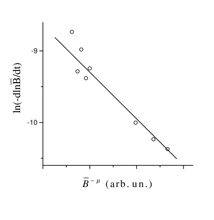
FIG. 8.: On the determination of the flux creep parameters from the experimental MO data on magnetic relaxation. ${\bar{B}}(t)$ is the remanent field in the central region of the bridge after switching off the external field 100 mT. The experimental dependence $\ln(-d\,\ln{\bar{B}}/dt)$ versus ${\bar{B}}^{\mu}$ with $\mu=1/7$ is fitted by a straight line according to Eq. (11).

In the relaxation experiment the sample was cooled down to 15 K in external magnetic field 100 mT, which is about $4B_{c}$ for our bridge. This high field ensures that the remanent state is fully penetrated by the current[4, 3]. Then the field was switched off and the time dependence of the remanent field was measured by MO technique in the time window 10¹-10³ s. From now on we focus on the peak field value $\overline{B}(t)$ observed in the central region of the bridge and averaged along its length. Instead of presenting of the relaxation of $\overline{B}$ directly, we chose to plot the logarithmic derivative $\ln(\partial\ln\overline{B}/\partial t)$ versus $\overline{B}^{\mu}$. The reason for this type of plot is the following. As was shown in Ref. [23], the pinning energy $U(x)$ remains almost the same locally at any stage in a relaxation process. That is a feature of a self-organized behavior of magnetic flux which is a consequence of the exponential dependence $v\propto\exp[-U(J)/kT]$. Since $U$ is almost constant $v$ varies also slowly in space, and therefore

$\displaystyle\frac{\partial B}{\partial t}\approx v\frac{\partial B}{\partial x}\,.$

We can roughly estimate $\partial B/\partial x$ as $\overline{B}/w$. Moreover, in a fully penetrated state $\partial B/\partial x\propto J$, and therefore, $J\propto\overline{B}$. This approximation together with Eq. (8) yields

$$\ln\left(-\frac{\partial\ln\overline{B}}{\partial t}\right)\approx\ln\left[\frac{v_{0}}{w}\exp\left(\frac{U_{c}}{kT}\right)\right]-\frac{\text{const}}{\overline{B}^{\mu}}.$$ (11)

The experimental quantity $\ln\left(-\partial\ln\overline{B}/\partial t\right)$ is plotted as a function of $\overline{B}^{-\mu}$ in Fig. 8. The experimental points show a nearly linear dependence, and the line representing the best fit is also shown. From the fit we obtain $v_{0}\,\exp(U_{c}/kT)\approx 10^{24}$ m/s. Assuming $v_{0}$=10 m/s (see, e.g., Ref. [22]) we estimate the pinning energy as $U_{c}=(50-55)\,kT\approx 0.08$ meV for $T=15$ K which is a quite reasonable value[30]. The other free parameter, the sheet current density $J_{cp}$, was chosen to provide the best agreement of results of flux creep simulations with experimental profiles shown in Fig. 3. It is interesting to compare the chosen value $J_{cp}=1.45\times 10^{3}$ A/cm with the critical sheet current density $J_{c}$ determined by fitting the same experimental data to the CSM. We found that $J_{c}\approx 0.37J_{cp}$. For this current density, the effective barrier $U_{\text{eff}}=U_{c}\left[\left(J_{cp}/J_{c}\right)^{\mu}-1\right]$ appears substantially lower than $U_{c}$, about $0.15\,U_{c}\approx 8\,kT$. It is worth noting that variation of $\mu$ in the range 1/7-1/3 has minor effect both on the calculated profiles $B(x)$ and on the relation $U_{\text{eff}}\approx 8\,kT$.

B Results

Let us first discuss general results of flux creep simulations. Time evolution of the profiles of current density and magnetic field under applying and switching off a transport current with density $J=0.26\,J_{cp}$ is shown in Fig. 9. The time dependence of the transport current was chosen as shown in Fig. 1 in accordance with the experimental procedure. For simplicity, only the case of zero external field is considered. Since all the distributions are symmetric in this case, we discuss the profiles for one half of the bridge.

The various curves in Figs. 9(a,b) correspond to different times as marked in Fig. 1. The profiles (1-4) corresponding to current-carrying states are very similar to the ones expected from the CSM. It is interesting to note that though the transport current did not change from the instant 1 to 2, the curves 1 and 2 in Fig. 9b differ substantially. Though both can be described by CSM-profiles, they correspond to different values of $J_{c}$. In particular, the transition from the curve 1 to 2 corresponds to $J_{c}$ decreasing in time. Time dependence of effective $J_{c}$ can be seen also from the curves 3 and 4 for the remanent state after current. A possibility to interpret experimental time evolution of magnetic flux profiles by the CSM with time-dependent $J_{c}$ has been previously demonstrated in Ref. [31]. An additional feature of calculated profiles in the remanent state is a peak of “negative” current density located not far from the bridge edge (cf. with Ref. [23]) – see curves 3 and 4 on Fig. 9b. The peak’s position corresponds to the annihilation zone where $B(x)$ changes its sign. This peak is a direct consequence of continuity

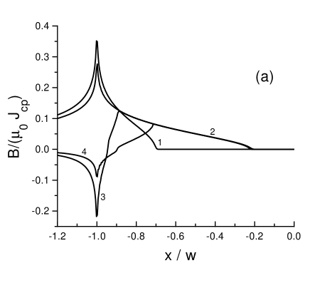
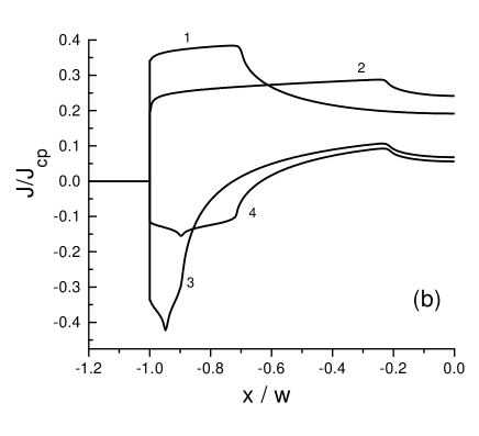
FIG. 9.: Results of flux creep simulation for $J/J_{cp}=0.26$ A. Evolution of profiles of the magnetic field (a) and the current density (b) in the strip plane for the time variation of the transport current shown in Fig. 1. Profiles (a) and (b) correspond to different times marked as different points in Fig. 1.

of the flux flow. Indeed, in the region of low density of flux lines their velocity (determined by the ratio $J/J_{cp}$) should be large to keep the flux flow continuous.

The dashed line in Fig. 10 is a result of our simulations of the magnetic field profile for $I=0.75\,I_{c}$ at $t=35$ ms after switching on the current. This time delay corresponds to the center of the plateau in the time dependence of the transport current, see Fig. 1, so it was the time when the MO images were recorded. The profile was calculated from the simulated current distribution using Eq. (1). In a similar way the flux profile for the remanent state ($t=30$ s) was calculated. The result is shown Fig. 5. It is clear that flux creep provides deeper penetration of the flux into the inner regions in agreement with the experiment.

For the current-carrying state, Fig. 10, the agreement is fairly good except two minor discrepancies. First, the experimental peaks at the bridge edges are less than the ones predicted both by the CSM and by our simulations. This is a rather general feature (cf. with Ref. [5]) which is probably originated from the finite thickness of the indicator film (in our case 5 $\mu$m), as well as from imperfection of the edges. Another discrepancy observed outside the bridge, is obviously related to contact currents. Indeed, Eq. (4) is based upon the assumption that the external field is small[21] and homogeneous. However, the field generated by the current in the contacts is actually inhomogeneous in $x$ direction, and far from the bridge it is significantly different from the one in its central part.

For the remanent states after current $I$, the account of flux creep provides good agreement with the experiments for $I\leq 4.16$ A, Fig. 5. However, at larger currents the experimental behavior of the trapped flux is qualitatively different. Indeed, both critical state and flux creep models predict monotonous dependence of the trapped flux on the current. Non-monotonous experimental dependence can serve as an indirect indication that some non-equilibrium process is responsible for the flux distributions observed after large currents.

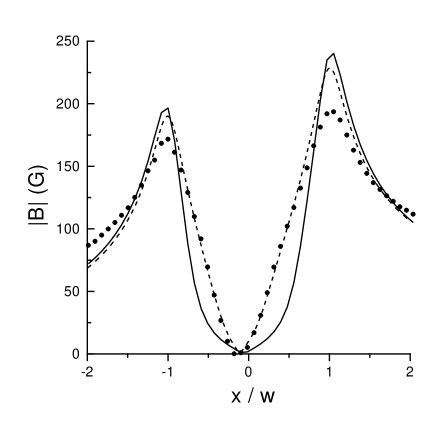
FIG. 10.: Profiles of the absolute value of perpendicular magnetic field induced by transport current $I=0.75I_{c}$ at the distance $h=8\ \mu$m above the sample. Dots – experiment, solid line – calculations along CSM, Eqs. (4),(1), dashed line – results of flux creep simulation. It is clearly seen that the flux creep leads to a deeper penetration of flux comparing to the CSM, in agreement with experiment.

We believe that formation of the remanent state after very large currents is strongly influenced by heating effects. As well-known, energy dissipation due to vortex motion facilitates more intensive motion. As a result, macroscopic avalanche-like flux redistributions (flux jumps)[32, 33, 34, 35, 36] can take place. Unfortunately, the works we are aware of are focused on the flux jumps in the case of applied magnetic field and slab geometry. We believe that the case of a remanent state in a strip after transport current requires a special theoretical treatment. Furthermore, the flux motion obviously takes place through narrow channels of weak pinning. Consequently, the energy dissipation is substantially inhomogeneous that should be taken into account in the estimates of local temperature. We plan special experiments, as well as the proper theoretical analysis as a subject of a future work.

To get a hint why the heating in the remanent state might be different from the one in the current-carrying state, we have compared the power dissipation. According to the estimates, the power dissipation due to vortex motion is larger in the current-carrying state. However, in the remanent state there is an extra source for dissipation – vortex-antivortex annihilation. Due to this contribution, the total power dissipation in the annihilation zone can be larger than that in the current-carrying state. Consequently the remanent state can be more unstable with respect to temperature fluctuations that the current-carrying one. It should be noted that a special behavior of vortices in the vicinity of the annihilation zone in the remanent state have already been addressed in literature. The most unusual feature is meandering instability of flux front and its turbulent relaxation observed in very clean single crystals[37]. The heat release in the annihilation zone is suggested as a probable explanation of this phenomenon. Another explanation is based upon the concept of magnetic field concentration inside the bend of a current line[38]. Furthermore, as discussed in Ref. [23], near the annihilation zone, a special behavior of flux creep can be expected. It is argued that under certain assumptions about $B$-dependence of the pinning energy, the presence of the annihilation zone destroys the normal course of flux creep in the whole sample.

Another possible source of an instability might be an additional heat release in the contact pads. However, according to the estimate given in Sec. IIA, the heat release in contact regions is negligible. This conclusion is confirmed by the fact that the bridge burn-out took place in its central part.[39]

V Conclusion

Measurements of magnetic flux distribution in a HTSC strip with transport current, as well as in the remanent state, are performed by magneto-optical method. The experimental results are compared with predictions of the critical state model for a strip geometry and with computer simulation of flux penetration in the flux creep regime. In the current-carrying state, the agreement was satisfactory. Simulation of flux creep predicts slightly deeper flux penetration than the CSM in agreement with experiment. In the remanent state after transport current, the CSM fails to explain the experimental results. Our simulations of flux creep allow to describe the flux profiles after relatively small current, $I\leq 0.7I_{c}$. At larger currents the total trapped flux appears substantially less than predicted by the flux creep simulations, and it decreases with increasing $I$. Excessive power dissipation in the annihilation zone can be an explanation of these experimental results.

Additional experiments and elaborated theoretical models for the remanent state are under development. We believe that an important information can be obtained from time-resolved studies of remanent state nucleation. The conditions for nucleation of macroscopic flux jumps is also a subject for future theoretical investigation.

- [1] C. P. Bean, Phys. Rev. Lett. 8, 250 (1962).
- [2] W. T. Norris, J. Phys. D: Appl. Phys. 3, 489 (1970).
- [3] E. H. Brandt, M. Indenbom, Phys. Rev. B 48, 12893 (1993).
- [4] E. Zeldov, J. R. Clem, M. McElfresh, and M. Darwin, Phys. Rev. B 49, 9802 (1994).
- [5] T. H. Johansen, M. Baziljevich, H. Bratsberg, Y. Galperin, P. E. Lindelof, Y. Shen, and P. Vase, Phys. Rev. B 54, 16 264 (1996).
- [6] T. Shuster, H. Kuhn, E.H. Brandt, M. Indenbom, M. Koblichka, M. Konczykowski, Phys. Rev. B 50, 16684 (1994).
- [7] R.J. Wijngaarden, H.J.W. Spoelder, R. Surdeanu, R. Griessen, Phys. Rev. B, 54, 6742 (1996).
- [8] A. A. Polyanskii, A. Gurevich, A. E. Pashitski, N. F. Heinig, R. D. Redwind, J. E. Nordman, and D. C. Larbalestier, Phys. Rev. B 53, 8687 (1997).
- [9] V. K. Vlasko-Vlasov, M. V. Indenbom, V. I. Nikitenko, A. A. Polyanskii, R. L. Prozorov, I. V. Grakhov, L. A. Delimova, I. A. Liniichuk, A. V. Antonov, and M. Y. Gusev, Superconductivity 5, 1582 (1992).
- [10] M. V. Indenbom, A. Forkl, H. Kronmüller, and H.-U. Habermeier, Journ. of Superconductivity 6, 173 (1993).
- [11] T. H. Schuster, M. R. Koblischka, B. Ludescher, W. Gerhäuser, and H. Kronmüller, phys. stat. sol. (a) 130/2, 429 (1992).
- [12] M. D. Johnston, J. Everett, M. Dhalle, A. D. Caplin, J. C. Moore, S. Fox, C. R. M. Grovenor, G. Grasso, B. Hensel, and R. Flükiger, In: “High-Temperature Superconductors: Synthesis, Processing, and Large-Scale Applications”, Ed. by U. Balachandran, P. J. McGinn, and J. S. Abell (TMS, 1966) p. 213.
- [13] U. Welp, D. O. Gunter, G. W. Crabtree, J. S. Luo, V. A. Maroni, W. L. Carter, V. K. Vlasko-Vlasov, V. I. Nikitenko, Appl. Phys. Lett. 66, 1270 (1995).
- [14] A. E. Pashitski, A. Polyanskii, A. Gurevich, J. A. Parrell, and D. C. Larbalestier, Appl. Phys. Lett. 67, 2720 (1995).
- [15] A. Oota, K. Kawano, T. Fukunaga, Physica C 291, 188 (1997).
- [16] J. Herrmann, N. Savvides, K.-H. Muller, R. Zhao, G. McCaughey, F. Darmann, M. Apperley, Physica C 305, 114 (1998).
- [17] S. F. Karmanenko, V. Y. Davydov, M. V. Belousov, R. A. Chakalov, G. O. Dzjuba, R. N. Il’in, A. B. Kozyrev, Y. V. Likholetov, K. F. Njakshev, I. T. Serenkov, O. G. Vendic, Supercond. Sci. Technol. 6, 23 (1993).
- [18] P. C. Michael, J. U. Trefny, and B. Yarar, J. Appl. Phys. 72, 107 (1992).
- [19] R. P. Huebener, in: Advances in Electronics and Electron Physics, 70, ed. by P. W. Hawkes (Academic, New York, 1988), p. 1.
- [20] L. A. Dorosinskii, M. V. Indenbom, V. I. Nikitenko, Yu. A. Ossip’yan, A. A. Polyanskii, and V. K. Vlasko-Vlasov, Physica C 203, 149 (1992).
- [21] The sufficient condition for Eq. (4) to be valid can be written as . The upper estimate for is a field generated by two parallel semi-infinite wires carrying the current in the middle of the segment connecting their ends, see Fig. 2. Thus , where is the bridge length while is a numerical factor. Our experimental data are compatible with . Since inequality appears met.
- [22] H. G. Schnack, R. Griessen, J. G. Lensink, C. J. van der Beek, and P. H. Kes, Physica C 197, 337 (1992).
- [23] L. Burlachkov, D. Giller, and R. Prozorov, cond-mat/9802076.
- [24] W. Wang, J. Dong, Phys. Rev. B 49, 698 (1994).
- [25] A. Gurevich and E. H. Brandt, Phys. Rev. B 55, 12706 (1997).
- [26] Th. Schuster, H. Kuhn, and E. H. Brandt , S. Klaumunzer, Phys. Rev. B 56, 3413 (1997).
- [27] G. Blatter, M.V.Feigel’man, V.B.Geshkenbein, A.I.Larkin, and V.M. Vinokur, Rev. Mod. Phys. 66, 1125 (1994).
- [28] Y. Yeshurun, A. P. Malozemoff, and A. Shaulov, Rev. Mod. Phys. 68, 911 (1996).
- [29] M.V.Feigel’man, V.B.Geshkenbein, A.I.Larkin, and V.M. Vinokur, Phys. Rev. Lett. 63, 2303 (1989).
- [30] C. W. Hagen, R. Griessen, Phys. Rev. Lett. 62, 2857 (1989).
- [31] M. McElfresh, E. Zeldov, J.R. Clem, M. Darwin, J. Deak, and L. Hou, Phys. Rev. B 51, 9111 (1995).
- [32] A. V. Gurevich and R. G. Mints, Rev. Mod. Phys. 59, 941 (1987).
- [33] M. E. McHenry, H. S. Lessure, M. P. Maley, J. Y. Coulter, I. Tanaka, H. Kojima, Physica C 190, 403 (1992).
- [34] M. E. McHenry, R. A. Sutton, Prog. in Mat. Sci. 38, 159 (1994).
- [35] K. H. Müller and C. Andrikidis, Phys. Rev. B 49, 1294 (1994).
- [36] R.G.Mints, E.H. Brandt, Phys. Rev. B, 54, 12421 (1996).
- [37] M. R. Koblischka, T. H. Johansen, M. Baziljevich, H. Hauglin, H. Bratsberg, and B. Ya. Shapiro, Europhys. Lett. 41, 419 (1998).
- [38] V. K. Vlasko-Vlasov, U. Welp, G. W. Crabtree, and D. Gunter , V. Kabanov and V. I. Nikitenko, Phys. Rev. B 56, 5622 (1997).
- [39] M. E. Gaevski, T. H. Johansen, Yu. Galperin, H. Bratsberg, A. V. Bobyl, D. V. Shantsev, and S. F. Karmanenko, Appl. Phys. Lett. 71, 3147 (1997).