Frequency-Dependent Response near the Glass Transition: A Theoretical Model

Abstract

We propose a simple dynamical model for a glass transition. The dynamics is described by a Langevin equation in a piecewise parabolic free energy landscape, modulated by a temperature dependent overall curvature. The zero-curvature point marks a transition to a phase with broken ergodicity which we identify as the glass transition. Our analysis shows a connection between the high and low frequency response of systems approaching this transition.

The glass transition in both spin systems and supercooled liquids is heralded by anomalously slow relaxations[1, 2]. Mode-coupling theory provides a framework for analyzing the dynamics of the supercooled state[1] and has been remarkably successful in predicting the general features of relaxations in a highly viscous supercooled liquid. However, detailed comparisons with experiments indicate that a complete description of the glass transition is still lacking. An alternative description of glass formation relies on the presence of multi-valleyed free energy surfaces[3] and the activated dynamics resulting from the presence of these traps[4].

Recent experiments indicate that the approach to the glass transition has some universal features[5] when viewed in terms of the frequency-dependent response of the system. In both supercooled liquids[5] and spin glasses[6], a frequency-independent behavior at high frequencies and the presence of three distinct regimes in the relaxation spectrum seem to be generic features of the approach to the glass transition. This behavior is different from that observed near a critical point where the high-frequency response is thought to be uninteresting[7]. In this paper, we present a dynamical model which provides a good description of the frequency-dependent response near the glass transition.

Dynamics of systems approaching the glass transition have been modeled by random walks in environments of traps [4]. What distinguishes our model is the presence of an overall curvature modulating the landscape of the traps, and the description of the dynamics $within$ the traps. The curvature is introduced to model the coupling between a set of variables which are inherently frustrated and another which tends to remove the degeneracy leading to the possibility of a unique global minimum and many local minima of the free energy[8]. An example of such variables could be the spins and strain fields in a spin glass[9] or a frustrated antiferromagnet[8], or a local orientational order parameter in a liquid coupled to local distortions of the liquid[10]. The vanishing of the overall curvature is identified in our model with the glass transition. This is reminiscent of models where the glass transition is associated with an instability[11] or an avoided critical point[12].

The presence of the curvature ($R$) ensures that an equilibrium distribution exists for all $R>0$. At $R=0$, this distribution becomes non-normalizable and there is a transition to a phase with broken ergodicity[4, 13]. As this glass transition is approached, the relaxation within the traps leads to the appearance of a regime in frequency space, $R<<\omega\leq a/R$, where the response is essentially frequency independent. The parameter $a$ defines how fast $R$ approaches zero as the glass transition temperature is approached. At frequencies smaller than a cutoff, ${\omega}_{c}\rightarrow 0$ as $R\rightarrow 0$, the response is described by a power law with a positive exponent. The exact relationship between ${\omega}_{c}$ and $R$ and the exponent of the power law depend on specific characteristics of the model. In particular, we find that if there is no correlation between the depth of a trap and its position inside the megavalley, the peak approaches zero algebraically and is accompanied by a flattening out of the low-frequency response. This is reminiscent of the observations in spin glasses[6]. If, on the other hand, correlations are introduced such that the deeper subwells are positioned further away from the center of the megavalley, then the shift of the peak follows a Vogel-Fulcher type law and there is no evolution of the low-frequency power law: a scenario that is reminiscent of the behavior of supercooled liquids[5].

Fig 1 shows a set of relaxation spectra for the model with no correlations. It demonstrates clearly that the low frequency power law approaches zero as the curvature is reduced and that there is a high-frequency regime, beyond the peak which grows and becomes flatter as the curvature is reduced. Whether or not the high-frequency cutoff to the power law ($\omega\simeq a/R$) is visible within the same window as the peak ($\omega\simeq R$) depends on the parameter $a$. The inset shows that there are three distinct frequency regimes and these have a striking resemblance to observations in spin glasses[6].

Each trap, or valley, is represented by a subwell and characterized not only by the time it takes to escape from it but also by its internal relaxation time. All subwells in the free-energy as well as the overall megavalley are assumed to be parabolic (cf Fig. 2). Each subwell is parameterized by its curvature $r_{n}$, width $\Delta_{n}$, position of the center $\phi^{0}_{n}$ and position of the minimum $C_{n}$. The set of $\{C_{n}\}$ is fixed by the requirement that free energy $F(\phi)$ is a continuous function. To simplify the picture even further, we set all $\Delta_{n}=\Delta$ which then automatically fixes $\phi^{0}_{n}=n\Delta$. The curvatures are taken to be independent random variables picked from a distribution $P(r,n)$. This defines a free-energy functional;

$$F(\phi)={1\over 2}R\phi^{2}+{1\over 2}\sum_{n=-\infty}^{\infty}\mu_{n}\Bigl{\{}r_{n}(\phi-\phi^{0}_{n})^{2}+C_{n}\Bigr{\}},$$ (1)

where $\mu_{n}$ is the support of the $n$-th subwell.

The dynamics is modeled by relaxation in this free-energy surface and is defined by the Langevin equation

$${\partial\phi\over\partial t}=-R\phi-\sum\mu_{n}r_{n}(\phi-\phi^{0}_{n})+\eta(t),$$ (2)

where $\eta$ is a Gaussian noise with zero average and variance $<\eta(t)\eta(t^{\prime})>=\Gamma\delta(t-t^{\prime})$. The temperature scale is set by $\beta=\Delta^{2}/\Gamma$ and it is useful to introduce the “effective” curvature of a subwell; $R_{n}=R+r_{n}$. Specific features of the distribution $P(r,n)$ affect the detailed nature of the response. The assumption that the curvature of each subwell is uncorrelated with its position, $P(r,n)\sim P(r)$ is the easiest to implement and is the scenario that we examine in detail. The changes occurring due to correlations are then discussed in the light of these calculations.

A natural candidate for $P(r)$ is an exponential distribution $P(r)=e^{-\beta_{0}r}/\beta_{0}$. This type of distribution has been observed in many spin-glass models[4], where it leads to power law distributions of escape times. Such distributions have also been observed in some Ising-like systems (without quenched disorder) which demonstrate glassy behavior[8]. It has been shown that, in absence of the overall curvature, $\beta=\beta_{0}$ is the temperature where the system falls out of equilibrium[4]. Our model has two characteristic temperature scales, one set by $\beta_{0}$ and the other by $R$.

Although Eq.(2) is piecewise linear inside each subwell, the long time evolution of the system is a non-uniformly biased random walk in a random environment and there is no exact solution to this problem. However, the existence of an equilibrium distribution can be proven rigorously. The equilibrium probability distribution is given by $\exp(-\beta F(\phi))$ as long as the integral of this function over $\phi$ remains finite[13]. A simple calculation shows that this integral diverges as $1/{(\beta_{0}-\beta){\sqrt{R}}}$. In the absence of the overall curvature the $1/{\sqrt{R}}$ factor gets replaced by the system size and the probability density diverges as $\beta\to\beta_{0}$[4]. As $R\to 0$, the system falls out of equilibrium and there is a change from exponentially decaying correlations to power-law correlations in time. This transition can be studied by analyzing the equilibrium correlation functions and the response functions associated with these through the fluctuation dissipation relation[7].

A non-zero overall curvature and the requirement that the subwells match at their boundaries, lead to a dependence of the effective barrier heights on the position and curvature of the subwells (cf inset of Fig. 2). The wells become asymmetric and the lower barrier of the $n$-th well is given by

$$\Delta F_{n}={R\over 2\rho_{n}}({1\over 2}-n\rho_{n})^{2},$$ (3)

where $\rho_{n}=R/R_{n}$. This expression is true for $n\rho_{n}<1/2$, otherwise $\Delta F=0$. Clearly, the dynamics in subwells $\Delta F>0$ and those with $\Delta F=0$ is very different. In fact, it is possible to talk about internal dynamics only when the internal relaxation time $(r_{n})^{-1}$ is shorter than the escape time, which is $\sim{\beta}\exp(\beta\Delta F_{n}(r))$. This suggests writing the correlation function, $C(t)$, as a sum of two components: internal relaxation and barrier crossing contributions from the wells with non-zero barriers and a “free relaxation” inside the megavalley coming from the subwells where the barriers have vanished due to the overall curvature. The weakest point in our analysis is the treatment of the free relaxation. In the absence of an exact solution, we have described this as simply a Debye response weighted by the effective number of barrier-less wells:

$$C(t) = C(t)^{trap}+C(t)^{free}$$ (4)

$$C(t)^{trap} = \sum_{n}\theta({1\over 2}-n\rho_{n})e^{-\beta F_{n}^{min}}\Bigl{(}{e^{-R_{n}t}\over R_{n}}+e^{-{t\over\beta}e^{-\beta\Delta F_{n}}}\Bigr{)}$$

$$C(t)^{free} = \sum_{n}\theta(n\rho_{n}-{1\over 2}){e^{-\beta Rn^{2}-Rt}\over R}.$$

In writing these expressions, we have used that fact that an equilibrium distribution exists and the probability of finding the system in subwell $n$ is given by the Boltzmann factor, $\exp({-\beta F_{n}^{min}})$, where $F_{n}^{min}$ is the minimum value of the free energy inside a subwell. Assuming that the local curvature and the position are uncorrelated, and estimating the contribution of the trapped and free relaxation from the “average” weights of barrier and barrier-less wells at each position $n$, leads to:

$$\bar{C}(t)^{trap}=\sum_{n}\int_{n\rho_{n}<1/2}{dr}P(r)e^{-\beta F_{n}^{min}}\Bigl{(}{e^{-R_{n}t}\over R_{n}}+e^{-{t\over\beta}e^{-\beta\Delta F_{n}}}\Bigr{)},$$ (5)

where the first term describes the internal relaxation within subwells and the second term describes activated processes. The free part can be written in a similar fashion.

One of the most interesting aspects of our model is the high-frequency response and the origin of this can be understood from an analysis of the limiting model where $R=0$ and $\beta\rightarrow{\beta}_{0}$[4]. In this limit, the hopping term in $C^{trap}$ becomes identical to the one analyzed in [4]. In frequency domain, the imaginary part of the susceptibility, $\chi^{{}^{\prime\prime}}(\omega)=\omega C(\omega)$, is known to grow as $\omega^{(\beta_{0}-\beta)/\beta}$ at small frequencies and decays at large $\omega$ as $1/\omega$. However, there is a new feature arising from the internal dynamics which drastically changes the high frequency behavior. The internal relaxation part of $\bar{C}^{trap}$ is given by

$$\bar{C}(\omega)^{trap,int}=\int_{r^{*}}^{\infty}{dr}{e^{-(\beta_{0}-\beta)r}\over\omega^{2}+r^{2}}.$$ (6)

As $\beta\to\beta_{0}$, the contribution of this term to $\chi(\omega)$ becomes $({\pi}/2-{\rm atan}(r^{*}/{\omega}))$; an extremely slowly decaying function of frequency which has a high-frequency cutoff $\simeq 1/(\beta-\beta_{0})$[14]. The total frequency-dependent response, therefore, behaves as $\omega^{(\beta_{0}-\beta)/\beta}$ for $\omega\to 0$ and is a slowly-decaying function at large frequencies. The free (Debye) part is not present in this model with $R=0$.

The overall curvature changes the effective barriers heights and therefore influences the response at both high and low frequencies. To simplify the analysis, we adopt a specific relationship between $R$ and $\beta_{0}$, and choose the temperature at which $R=0$ to be at $\beta_{0}$ in such a way that $a(\beta_{0}-\beta)=\beta_{0}\beta R$ and take $a=1$. The equilibrium relaxation spectra are then given by,

$$C^{trap}(\omega)=\sum_{n}e^{-\beta Rn^{2}}\int_{nR}^{\infty}{dr}e^{-(\beta_{0}-\beta)r}\Bigl{(}{1\over\omega^{2}+r^{2}}+{e^{-\beta\Delta F(r,n)}/\beta\over\omega^{2}+e^{-2\beta\Delta F(r,n)}/\beta^{2}}\Bigr{)}.$$ (7)

In this expression, the first term arises from the internal relaxation, and is identical to (6), except for the cutoff being determined by $R$. The second term is the “hopping” contribution, and can be rewritten, after a change of variables, as

$$\bar{C}(\omega)^{trap,hop}={1\over\beta^{2}}\sum_{n}e^{-\beta Rn^{2}}\int^{\exp(-\beta nR)}_{0}{dz}{z^{-1+\beta_{0}/\beta}\over\omega^{2}+z^{2}/\beta^{2}}.$$ (8)

The overall curvature enters through the upper cutoff in the integral, and as $R\to 0$, exhibits the slow dynamics discussed in the previous paragraph. There is a tradeoff between the hopping dynamics and free relaxation with the hopping contribution decreasing as $R$ increases and more and more wells become effectively “free”. The free part is given by,

$$\bar{C}^{free}(\omega)={1\over R^{2}+\omega^{2}}\sum_{n}e^{-\beta Rn^{2}}\int^{nR}_{0}{dr}e^{-\beta_{0}r},$$ (9)

and leads to a Debye spectrum with peak at $\omega=R$. Numerical results based on this description of the response are shown in Fig. 1. The contribution from the deep traps shows one essential characteristic of the model; the change in the high-frequency response accompanying the low-frequency changes as $R\to 0$. The inset demonstrates that the free part is responsible for the shift in peak frequencies and the appearance of an intermediate regime.

There are three different regimes of the response: low frequency power law, associated with hopping between different subwells; Debye-like peak coming from barrier-less relaxation and high frequency power law decay as a result of superposition of multiple single relaxation time processes. The weakest point in this construction is the intermediate, Debye contribution which in principle overlaps with both low and high frequency tails. This crossover region we expect to be very sensitive to all the approximations made. On the other hand, the low-frequency and high-frequency regimes are relatively insensitive to these approximations since they depend on processes related to deep subwells.

This picture is very similar to the experimentally observed response in spin glasses [6], with the response flattening out at both high and low frequency ends and the peak moving much slower than exponentially. In supercooled liquids, only the high frequency piece flattens out, and the peak shifts towards zero frequency according to a Vogel-Fulcher law[2, 5]. From the viewpoint of our model this difference can be ascribed to a difference in the nature of correlations in the two systems. In a structural glass, the crystalline state is the absolute global free-energy minimum. The subwells of our model correspond to metastable states and the megavalley represents the states accessible in the supercooled phase, with the crystalline minimum lying outside this region. This suggests a model where the depth of a subwell and its position are correlated and the deeper wells are situated further away from the minimum of the megavalley. A correlation in $P(r,n)$, of the form suggested above, leads to an upper cutoff in the distribution of barrier heights (cf Eq. (7)). This cutoff leads to a maximum escape time $t_{esc}\sim\exp({1/R}^{\alpha})$ where $\alpha>0$ is the exponent of a power law describing the correlation between the depth and the position of subwells. Beyond this time scale, there is only barrier-free motion in our model and, therefore, at frequencies lower than ${\omega}_{c}=(t_{esc})^{-1}$, we predict that $\chi(\omega)\sim\omega$ and there is no flattening out of the low-frequency response. The upper cutoff does not have a large influence on the response arising from the internal dynamics of the subwells. The high-frequency cutoff is still approximately given by $1/R$ as can be easily seen from Eq. (6).

In conclusion, we have demonstrated that the basic features of the relaxation spectra near the glass transition can be understood on the basis of a multivalleyed free-energy surface with an overall curvature which goes to zero at the glass transition. The spectrum crosses over from being pure Debye at large curvatures to one with three distinct regimes with an asymptotic high-frequency power law characterized by an exponent approaching zero as the curvature goes to zero. The model is also characterized by the distribution of curvatures of the subwells. Our analysis suggests that the relaxation spectra of spin glasses and structural glasses can be described by the same underlying model with different correlations in the distribution of subwells.

The original motivation for constructing this model came from observations in a frustrated spin model without quenched disorder[8] whose phenomenology is remarkably similar to structural glasses. Simulations of this model indicated a free-energy surface with an overall curvature and the vanishing of this curvature was accompanied by the appearance of broken ergodicity and “aging”[8]. This same model also showed a power-law distribution of trapping times in the subwells[8]. This spin model can, therefore, be viewed as a microscopic realization of the dynamical model presented here. Since it can also be viewed as a model for real glasses, further studies of this model should lead to an understanding of the connection between spatial inhomogeneities and the anomalous relaxations near a glass transition and clarify the relevance of our dynamical model to real glasses.

***

The authors would like to acknowledge the hospitality of ITP, Santa Barbara where a major portion of this work was performed. This work has been partially supported by NSF-DMR-9520923.

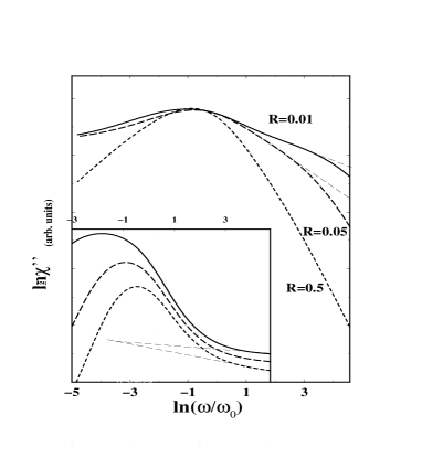
Fig. 1.–: Contribution of deep traps to the imaginary part of susceptibility, $\chi^{{}^{\prime\prime}}(\omega)$, for the model with no correlations, calculated using Eq. (7), for different values of $R$. The peak intensities have been matched. $\omega_{0}$ is a microscopic frequency scale determined by the parameters of the model. The inset shows the full relaxation spectra, including the contribution from the “free” subwells for $R=$ 0.1, 0.05 and 0.01. It is seen that the free part is responsible for the shift of the peak and the appearance of an intermediate regime. The long-dashed lines show the high-frequency power law extending up to $\omega\simeq a/R$. The parameter $a=1$ in the main figure but $a=100$ in the inset.

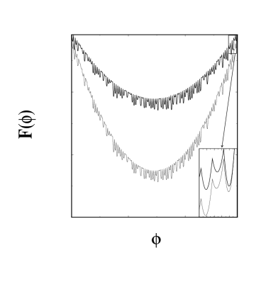
Fig. 2.–: Free energy landscape for two different values of $R$ with a fixed distribution of $\{r_{n}\}$. The inset shows how the overall curvature modifies the heights of the barriers between the subwells.

References

- [1] U. Bengtzelius, W. Gotze and A. Sjolander, J. Phys. C 17, 5915, 1984; W. Kob, Report no. cond-mat/9702073 and references therein.
- [2] M. D. Ediger, C. A. Angell and Sidney R. Nagel, J. Phys. Chem 100, 13200 (1996)
- [3] See, for example, F. H. Stillinger, Science 267, 1935 (1995)
- [4] C. Monthus and J. P. Bouchaud, J. Phys. A: Math. Gen. 29, 3847 (1996).
- [5] P. K. Dixon et al, Phys. Rev. Lett 65, 1108 (1990); N. Menon and S. R. Nagel, Phys. Rev. Lett 74, 1230 (1995).
- [6] D. Bitko et al, Europhys. Lett. 33, 489 (1996).
- [7] Nigel Goldenfeld, Lectures on Phase Transitions and the Renormalization Group, (Addison Wesley, New York, 1992).
- [8] Lei Gu and Bulbul Chakraborty, Mat. Res. Symp. 455, 229 (1997), and to be published.
- [9] Z. Y. Chen and M. Kardar, J. Phys. C 19, 6825 (1986).
- [10] S. Dattagupta and L. Turski, Phys. Rev. B 47, 1222 (1993).
- [11] A. I. Mel’cuk et al, Phys. Rev. Lett. 75, 2522 (1995).
- [12] S. A. Kivelson et al, J. Chem. Phys. 101, 2391 (1994).
- [13] J. Zinn-Justin,Quantum Field Theory and Critical Phenomenon, (Oxford, England, 1989).
- [14] The lower cutoff is introduced to ensure that one can define an internal relaxation process. This arbitrary cutoff is necessary only for and does not affect the high-frequency behavior.