Critical properties of a three dimensional p-spin model

Abstract

In this paper we study the critical properties of a finite dimensional generalization of the $p$-spin model. We find evidence that in dimension three, contrary to its mean field limit, the glass transition is associated to a diverging susceptibility (and correlation length).

I Introduction

Two different transition mechanisms are known in spin glass mean-field theory [1, 2], according to the form of the random Hamiltonian. In some models, like the infinite range Sherrington-Kirkpatrick (S-K) model for spin glasses, there is a second order glassy transition with diverging spin-glass susceptibility and continuous replica symmetry breaking. In other models, whose prototype is the Random Energy Model, the transition is first order with a Gibbs-Dimarzio like entropy crisis. Other examples of models with the second type of behaviour are spin models with p-spin interaction, with $p>2$, both for Ising spins and for spherical spins.

Numerical simulations indicate that the first type of mechanism describes the ergodicity breaking transition of finite dimensional spin glasses [3]. The second mechanism is more appropriate to describe the behavior of structural glasses[4]. The passage from mean-field to finite dimension is in both cases highly non trivial. Despite many progresses [5] the problem of including fluctuations in the description of the finite dimensional spin glass transition is far from being achieved. For that reason the test of the mean-field picture has been left in the last 15 years to the numerical study of the Edwards-Anderson model, which admits the SK as infinite dimensional limit.

Strangely enough there are only few numerical studies of finite dimensional spin models that could have a transition homologous to the mean-field discontinuous transition. Given the relevance of this transition to structural glasses, the study of such finite dimensional models is of primary importance.

Up recently,to our knowledge, the only studies appeared in the literature, are these references [6] and [7]. In reference [7] it was proposed a generalization of the $p$-spin model which presents a phenomenology reminiscent to that of structural glasses. However, the difficulty to decide about the existence of a phase transition and the presence of a spurious symmetry, makes necessary to resort to better conceived models without spurious effects.

In this paper we introduce, and study numerically, a finite dimensional model with $N$ spin per sites and $p$-spin interactions, that for all dimensionality tends to a mean-field behaviour for $N\to\infty$. As it happens in ordinary field-theory, this large $N$ approach is complementary to the high-dimensionality approach. We study this model for $p=4$ in $D=3$. A complementary study of the same model (still for $p=4$ and $D=3$) in the low temperature regime can be found in ref. [8]. Some numerical simulation of the $p=3$ model for $D=4$ can be found in ref. [9].

II A finite dimensional $p$-spin model

The long range p-spin model [10] is soluble and its Hamiltonian is given by

$$H=-\sum_{i_{1}<...<i_{p}}^{1,N}J_{i_{1},...,i_{p}}S_{i_{1}}...S_{i_{p}},$$ (1)

where the variables $J$ are random with zero average and variance $1/N^{(p-1)}$ (the same result is obtained for Gaussian distributed variables and in the case $J=\pm 1/N^{((p-1)/2)}$) and the spins are Ising variables (also the spherical case is soluble).

This Hamiltonian can be generalized in many ways in finite $D$. The way we follow in this paper is the following: we consider a $D$ dimensional square lattice with $N$ Ising spins $S_{x}^{\alpha}$ ($\alpha=1,...,N)$ in each site $x$ of the lattice. For any given couples of nearest neighbour sites there are $(2N)!/p!(2N-p)!$ possible groups $g$ of p-spins. We consider the product of all the spins in each group, and we couple them with a random variable $J_{g}$. The resulting Hamiltonian, with transparent notation, is

$$H=-\sum_{<x,y>}\sum_{g\in(x,y)}J_{g}\prod_{\mu\in g}S_{\mu},$$ (2)

where we have relabeled the spins. The $J_{p}$ are chosen independently from link to link and group to group and are equal to $\pm 1$ with probability $1/2$. The mean field limit is recovered both for high dimension ($D\to\infty$) and finite $N$ or for large $N$ and finite $D$. Indeed it is possible to construct a loop expansion for the development in powers of $1/N$ [11]. In this paper we present a numerical study of the model in $D=3$ for low values of $N$ above the transition point.

We have simulated the physics of the model through Monte Carlo method with the Metropolis algorithm. We have studied in detail the cases $p=4$ and $N=3$ and 4. As we will see the results do not seem to depend qualitatively on $N$ in this range of $N$ (for $N=2$ and $p=4$ the model is isomorphic to the usual short range Edwards Anderson model for spin glasses).

In this first study of the model we discuss mainly three issues:

• The existence of a glass transition by means of the study of the thermodynamics of the model, through the behaviour of the energy and the entropy in simulations of “cooling experiments”.

• The behaviour of the time dependent auto-correlation function at equilibrium and the growing of the relaxation time as the glass transition is approached.

• The existence of a growing spin-glass correlation length.

Let us start with the discussion of cooling experiments. In figure 1 and 2 we show the energy as a function of the temperature for different cooling rates for $N=3$ and 4 respectively. The cooling rate $\kappa$ is equal to the inverse of the number of Monte Carlo sweeps done at each temperature. We recognize in both cases the typical curves of systems undergoing a glass transition, and remaining frozen below a cooling rate dependent freezing temperature. In the figure with $N=4$ we have plotted for comparison purposes the line corresponding to the first term of the high temperature expansion. We see that until quite near to the freezing the energy of the system remains close to that line. This is reminiscent to what happens in mean-field, where the line is followed up to the transition point.

In figure 3 we study the dependence of the energy on the cooling rate for the $N=4$ model for $T=2$ and $T=4$ as a function of the inverse cooling rate. The data are compatible with a power law relaxation of the kind $E(\kappa)=E_{\infty}+A\kappa^{u}$ with a temperature dependent exponent $u$. For instance a fit of the data for $T=2,4$ gives $E(\kappa)|_{T=2}=-65.8+11.6\times\kappa^{0.21}$ and $E(\kappa)|_{T=4}=-65.1+11.9\times\kappa^{0.23}$. This dependence contrasts with the much slower logarithmic dependence observed in real glasses and is the first sign of criticality in the system.

In the equilibrium regime (which is reached for sufficient long simulations) we can obtain free-energy and entropy integrating the data of the internal energy and taking into account that at infinite temperature the entropy per spin is $S(T=\infty)=\log 2$. The free-energy is reconstructed as

$$F=\log 2-T\int_{0}^{1/T}E(\beta){\rm d}\beta,$$ (3)

and from it the entropy, that we plot in figure 4. We observe that $S(T)$ behaves linearly in a wide range of temperatures suggesting the validity of the Gibbs-Di Marzio transition mechanism for this model. As we will see the model with $N=3$ seems to have a transition around $T=2.6$ while the linear extrapolation of the entropy vanishes only at $T\approx 1.8$. However it is not the total entropy, but the “configurational entropy” (associated to the number of possible metastable states) that should vanish at the transition.

We now turn to the more difficult question of the identification and characterization of the phase transition in the model. We have studied that issue limiting ourselves to the case $N=3$. The quantity over which we have concentrated is the overlap correlation length. We simulated two identical replicas in parallel ($\sigma$ and $\tau$), and after thermalization we measured the overlap correlation function:

$$G(x)={1\over N^{2}V}\sum_{i=1}^{V}\sum_{\alpha=1}^{N}\sum_{\beta=1}^{N}\sigma_{i}^{\alpha}\sigma_{i+x}^{\alpha}\tau_{i}^{\beta}\tau_{i+x}^{\beta}.$$ (4)

The spin glass susceptibility is defined as

$$\chi_{SG}=\int{\rm d}^{3}x\;G(x).$$ (5)

The data for the function $G(x)$ are shown in figure 5 for $T=3$, together with the the best fit of the form $G(x)=A/(x+1)^{1+\eta}\exp(-x/\xi)$ with $\eta=0$. We have done similar fits at different temperatures and in this way we have extracted the value of the correlation length. If we plot this correlation length as a function of the temperature (fig. 6) we see that the data are best fitted by the power form $\xi\approx(T-T_{c})^{\nu}$, with $T_{c}=2.62$ and $\nu=0.71$. However from figure 7 we see that the data are also well compatible with $\nu=2/3$ as one could expect from scaling arguments (see below).

Differently from mean field there is a correlation length growing in the system, that suggests a second order phase transition.

Similar conclusions also come from the analysis of the spin glass susceptibility, which grows of about a factor ten in the range $3<T<4.4$. The data, shown in figure 8 are roughly compatible with a power law divergence of the susceptibility as $\sim\xi^{2.4}$, which using the value $2/3$ for $\nu$ corresponds to $\chi_{SG}\approx(T-T_{c})^{\gamma}$ with $\gamma=1.6$. These values for the critical exponents $\gamma$ and $\nu$ are definitely different from those of the Edwards Anderson spin glass models: they are a factor 2-3 times smaller [3].

The last aspect that we have studied is the equilibrium relaxation, and the relation of the relaxation time with the correlation length. In figure 9 we show the time autocorrelation function

$$C(t)={1\over NV}\sum_{i,\alpha}\sigma_{i}^{\alpha}(t)\sigma_{i}^{\alpha}(0)$$ (6)

for various temperature for $N=4$. We see that a form $C(t)=A\exp(-(t/\tau)^{\beta})$ fits excellently the data. We extract from that the relaxation time $\tau$ (figure 10) and the exponent $\beta$ that we plot in figure 11.

We also done the same analysis for $N=3$ with similar results. It is interesting to plot $\tau$ versus $\xi$ which shows the compatibility of our data with the relation $\tau\sim\xi^{z}$ (see figure 12). This scaling form is at variance with the results of [7] for the other short range p-spin model we mentioned in the introduction, and experiments in structural glasses. The high value of $z$ we find. i.e. $z=8$ (which by coincidence is quite similar to the value in the Edwards Anderson spin glass model) implies a violent divergence of the correlation time near the transition and it is responsible of the large correlation time needed to reach thermalization.

The difference of behaviour with respect to the mean-field can be rationalized with the argument presented in the next section, which also implies $\nu=2/3$.

III A possible theoretical interpretation

The difference among the short range model and the homologous infinite range model (which can be solved in the mean field approximation) are quite striking. No precursor signs of the transition are present in the infinite range model and the spin glass susceptibility remains finite up to the transition point. Here we will present and argument which suggests that in short range models with quenched local disorder the spin glass susceptibility is divergent as in second order phase transitions.

The precise reasons for this discrepancy are not clear to us. The simplest scenario we have considered is the following. The disorder induces fluctuations in the local transition temperature. For a given region of radius $R$ centered around the point $x$ we can define and effective critical temperature $T_{R}(x)$. It is natural to assume that the $x$-dependent fluctuation of $T_{R}(x)$ is a quantity of order $R^{-D/2}$, i.e.

$$T_{R}(x)=T_{c}+\delta T_{R}(x)$$ (7)

with $\langle\delta T_{R}(x)^{2}\rangle\propto R^{D}$. At a given temperature $T$ the regions of size $R$ such that $T_{R}(x)>T$ are strongly correlated. The typical radius of these region increases as $(T-T_{c})^{2/D}$ suggesting therefore that $\nu=2/D$. This value of $\nu$ is peculiar for random systems. Indeed there are general arguments that show that for second order phase transitions disorder is relevant if $\nu\geq 2/D$ [12].

We also notice that the same value of $\nu$ can be obtained if we assume that the specific heat has a discontinuity at the phase transition as predicted by the mean field analysis. In other words we suppose that the specific heat exponent $\alpha$ is equal to zero. The usual scaling law $\alpha=2-D\nu$ implies the result $\nu=2/D$. This argument is suggestive, but the coincidence its prediction with the value of $\nu$ we find may be fortuitous of the dimension three. An investigation of the model in higher dimensions will give some information on the validity on this conjecture (numerical simulations in four dimensions for the $p=3$ model [9] suggest that in this case $\nu$ is around .5).

IV Conclusions

In this paper we have studied by Monte Carlo a finite dimensional version of the p-spin model. We find a scenario for freezing that mixes typical features of structural glasses, like strong cooling rate dependence of the low temperature energy, with features of second order phase transitions with power law growing of the correlation length and critical dynamics. This is a genuine finite dimensional effect due to the quenched disorder which can be understood qualitatively with the argument we have given. A full theoretical understanding should come from the inclusion of non-perturbative effects in the theory. The simulations of disordered finite dimensional analogous of systems with “one step replica breaking” is just at the beginning and much progress can be expected in the future.

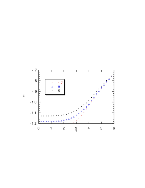
FIG. 1.: The energy for $N=3$ and three different values of the cooling rate $\kappa=2^{-5},2^{-8},2^{-17}$.

FIG. 2.: The energy for $N=4$ and three different values of the cooling rate ($2^{-5}$, $2^{-7}$, $2^{-12}$), together with the first term of the high temperature expansion. The curves stay close to the first term of the high temperature expansion until very close to where they fall off equilibrium.

FIG. 3.: The energy for $N=4$ as a function of the inverse cooling rate. From top to bottom $T=8,6,4,2$. The full lines are the power law fits discussed in the text.

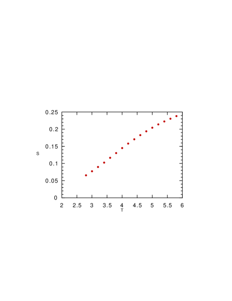
FIG. 4.: The entropy as a function of the temperature for $N=3$.

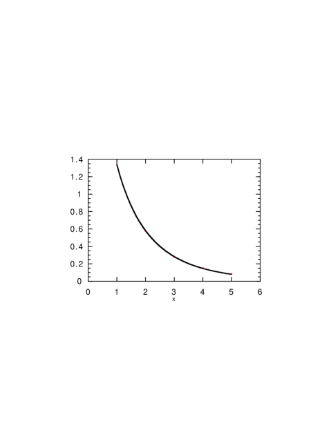
FIG. 5.: Overlap correlation function as a function of distance for $N=3$, $T=3$, together with the fit of the form $c(x)={A\over x+1}\exp(-x/\xi)$. The value of $\xi$ from the fit is $\xi=2.5$.

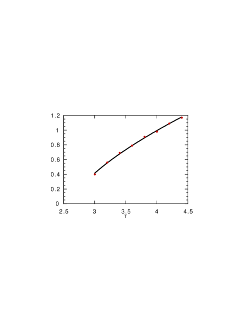
FIG. 6.: Inverse of the correlation length versus temperature for $N=3$ and fit $\xi^{-1}=(T-T_{c})^{\nu}$, $\nu=0.71$, $T_{c}=2.62$.

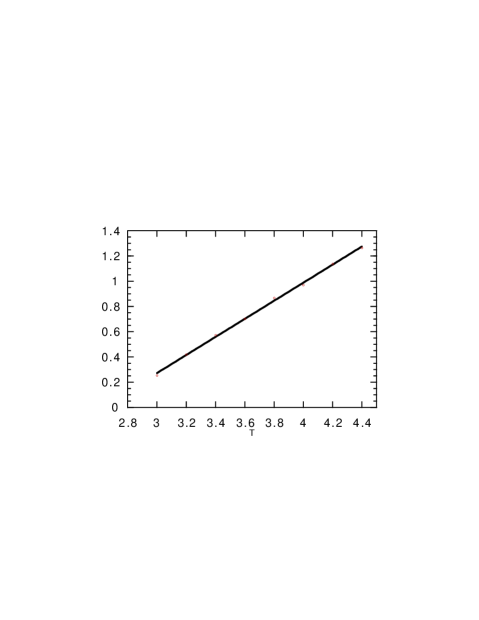
FIG. 7.: Correlation length $\xi$ to the power -2/3 versus temperature for $N=3$. The curve is a linear fit.

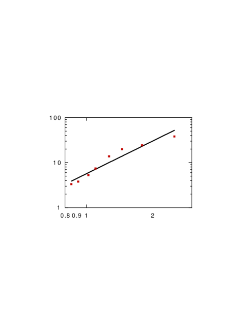
FIG. 8.: Spin glass susceptibility $\chi_{SG}$ versus $\xi$ for $N=3$ and the power best fit which gives $\chi\sim\xi^{2.4}$

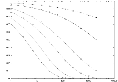
FIG. 9.: Time dependent auto-correlation function at equilibrium in the $N=4$ model for, from top to bottom, $T=5,6,7,8,9,10$ the lines are strctched exponential fits.

FIG. 10.: Relaxation time extracted from the autocorrelation function as a function of the temperature for $N=4$. The line is a power law fit $\tau=117.8\times(T-6.4)^{2}.1$.

FIG. 11.: Stretching exponent versus temperature for $N=4$. The line is a linear fit of the region $T<10$: $\beta=T\times 0.093-0.29$.

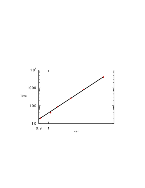
FIG. 12.: Relaxation time versus $\xi$ for $N=3$. The line is a power law fit with power $z=8$.

REFERENCES

- [1] M. Mezard, G. Parisi, and M.A. Virasoro, Spin Glass Theory and Beyond, World Scientific (1987).
- [2] A. P. Young (ed.), Spin Glasses and Random Fields (World Scientific, Singapore, 1997).
- [3] E. Marinari, G. Parisi and J.J. Ruiz Lorenzo, in ref. [2].
- [4] T.R. Kirkpatrick and D. Thirumalai, Phys. Rev. B 36, 5388 (1987); T.R. Kirkpatrick and P. G. Wolynes, Phys. Rev. B 36, 8552 (1987); a review of the results of these authors and further references can be found in T.R. Kirkpatrick and D. Thirumalai Transp. Theory and Stat. Phys. 24, 927 (1995).
- [5] C. De Dominicis and I. Kondor in ref. [2]
- [6] H. Rieger, Physica A184 (1992) 279, J. Kisker, H. Rieger and H. Schreckenberg, J. Phys. A (Math. Gen.) 27 (1994) L853.
- [7] D.Alvarez,S. Franz and F. Ritort Phys. Rev. B 54, 9756 (1996).
- [8] M. Campellone, B. Coluzzi and G. Parisi, cond-mat/9804291 Numerical study of a short-range p-spin glass model in three dimensions .
- [9] E. Marinari, C. Naitza, F. Zuliani, G. Parisi, M. Picco and F. Ritort, A general method to determine replica symmetry breaking transitions, preprint cond-mat/9802309.
- [10] The -spin model with Ising variables was studied in: E. Gardner, Nucl. Phys. B257 (FS14), 747 (1985). The version with spherical variables has been recently object of extensive study. A review of many results can be found in: A. Barrat, Preprint cond-mat/9701031 The p-spin spherical spin glass model unpublished.
- [11] M. Campellone, G. Parisi and P. Ranieri, Finite dimensional corrections to mean-field in a short range -spin glassy model, in preparation.
- [12] A.B. Harris, J. Phys. C 7, 677 (1974).