Semi-classical study of the Quantum Hall conductivity.

Abstract

The semi-classical study of the integer Quantum Hall conductivity is investigated for electrons in a bi-periodic potential $V(x,y)$. The Hall conductivity is due to the tunnelling effect and we concentrate our study to potentials having three wells in a periodic cell. A non-zero topological conductivity requires special conditions for the positions, and shapes of the wells. The results are derived analytically and well confirmed by numerical calculations.

P.A.C.S. number : 03.65.Sq , 73.50.Jt, 73.40.Hm , 73.20.Dx : electrons in low dimensional structures , 05.45.+b
key words: semi classical analysis, tunnelling effect, quantum Hall conductivity
AMS:81Q20 (WKB) 81S30 (phase space method) 82D20 (solids)

Frédéric Faure
Laboratoire de Physique Numérique des Systèmes Complexes, Université Joseph Fourier/CNRS, BP 166, 38042 Grenoble Cedex 9, France,
e-mail: faure@labs.polycnrs-gre.fr

Bernard Parisse
Institut Fourier, CNRS UMR 5582, 38402 St Martin d’Hères Cédex, France
e-mail: parisse@fourier.ujf-grenoble.fr

I Introduction

Some physical phenomenon happen to be expressible from topological properties of specific models. The integer Hall conductivity is one of them [9],[27]. In a simple model of non-interacting electrons moving in a two-dimensional periodic potential $V(x,y)$ subject to a uniform perpendicular magnetic field $B_{z}$ and a low electric field $E_{y}$, the Hall conductivity $\sigma_{xy}$ of a given filled Landau electronic band turns out to be proportional to an integer $C$:

$\displaystyle\sigma_{xy}=\frac{e^{2}}{h}C$

$C$ is the Chern index of the band, describing the topology of its fiber bundle structure [25],[15],[9],[8].
For a better understanding of this phenomenon, and to bring out the conditions of possible experimental measures, we investigate in this paper the value of $C$ as a function of the potential $V$. This is done by semi-classical methods, and the tunnelling effect appears to be the fundamental mechanism for a non-zero conductivity.
In the limit of high magnetic field $B_{z}$, the above model is mapped onto the well-known Harper model, by means of the Peierls substitution: the potential $V$ is considered as a perturbation of the cyclotron motion, and the averaging method of mechanics gives an effective Hamiltonian equal to the average of $V$ on the cyclotron circles. We neglect the coupling between the Landau bands [26]. For a high magnetic field, (hence for a small cyclotron radius,) this transformation gives an effective Hamiltonian $H_{eff}(q,p)\sim V(q,p)$, which is biperiodic in position and momentum (the phase space is a 2D torus), and an effective Planck constant $h_{eff}=hc/(eB)$. In this approximation, trajectories are the levels lines of $H_{eff}\sim V$. Furthermore, the expression of $h_{eff}$ shows that the high magnetic field regime corresponds to the semi-classical limit. This model will be the starting point of our study in the next section.
Quantum mechanics on the torus has been extensively used as a convenient framework to study basic properties of the semi-classical limit like quantum chaos ([18],[19],[20], [5]), or the tunnelling effect ([31, 32], [3]). For this purpose, a convenient tool is the Bargmann and Husimi representation which maps a quantum state to a function on the phase space. These representations are constructed with coherent states and will be recalled in section 3.
The new results presented in this paper are the conditions under which the tunnelling effect between three different wells can be responsible for a non-zero Hall conductivity. The conditions will be expressed by specifying the special positions the three wells must have inside a periodic cell.
It is worth mentioning that due to its topological aspect, it is natural to study the Chern index values in a generic situation, because topological properties are robust against perturbations. Secondly, in the generic ensemble of Hamiltonian under study, the integer values of the Chern indices are characterized by the position of the boundary where their value changes by one unit. These boundaries turn out to correspond to degeneracies in the spectrum [2]. We are therefore brought to study the generic location of these degeneracies, in the space of Hamiltonians. This is done in section 5 and 6.
Under reasonable assumptions on the tunnelling interaction in phase space, we find that the boundary of constant Chern index domain form ellipses in any generic two-dimensional subspace of the Hamiltonian’s space. These analytical results are well confirmed by numerical calculations in section 7.
These results extend previous work by the first author for the Hall conductivity resulting from the tunneling effect between two wells in a given periodic cell ([10], [11]). Although the methods looks similar, calculations and results are quite different.

II Quantum mechanics on the torus

A Classical dynamics on the torus

Let us consider a one-degree of freedom Hamiltonian (hence an integrable dynamics), periodic both in position $q$ and momentum $p$, with respective periods $Q$ and $P:$

$$H(q,p)=H(q+Q,p)=H(q,p+P)$$ (1)

The function $H(q,p)$ can be decomposed into its Fourier series:

$$H(q,p)=\sum_{n_{1},n_{2}\in Z^{2}}c_{n_{1},n_{2}}\exp(i2\pi n_{1}\frac{q}{Q})\exp(i2\pi n_{2}\frac{p}{P})$$ (2)

This decomposition will be used for numerical computations, but is not essential for the theoritical part of this work.

Since $H$ is a real valued function, the complex coefficients $c_{n_{1}n_{2}}$ must satisfy:

$\displaystyle c_{n_{1},n_{2}}=\bar{c}_{-n_{1},-n_{2}}\in I\!\!\!\!C,\quad(n_{1},n_{2})\in Z\!\!\!Z^{2}$

The trajectories $q(t),p(t)$ evolve on the plane, but because of periodicity, they can be considered as trajectories on the Torus $T_{qp},$ obtained by identifying the opposite sides of the cell $[0,Q]\times[0,P].$

For example, the trajectories of the Harper Hamiltonian

$$H(q,p)=-\cos(2\pi\frac{q}{Q})-\frac{1}{2}\cos(2\pi\frac{p}{P})$$ (3)

are displayed in figure 1, p. 1. Some energy levels are contractibles, others are not.

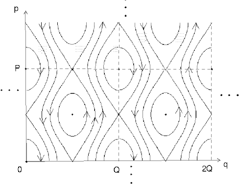
FIG. 1.: Trajectories of the Harper model (3).

B Quantum mechanics on the torus

The Hilbert space of a particle with one-degree of freedom is $L^{2}(I\!\!R)$, with the fundamental operators of position $\hat{q}$ and momentum $\hat{p}$ acting on a wave function $\psi(x),$ also noted $|\psi>.$

We now choose a symmetric quantization procedure: to the classical Hamiltonian $H$, we associate the quantum Hamiltonian:

$\displaystyle\hat{H}=\sum_{n_{1},n_{2}\in Z^{2}}\frac{1}{2}c_{n_{1},n_{2}}\exp(i2\pi n_{1}\frac{\hat{q}}{Q})\exp(i2\pi n_{2}\frac{\hat{p}}{P})+\mbox{hermitian conjugate}$

We denote by $\hat{T}_{Q}$ [respectively $\hat{T}_{P}$] the translation operator by one period. $\hat{T}_{Q}$ translates by $Q$ a wave function $\psi(x)$ and $\hat{T}_{P}$ translates its Fourier transform $\hat{\psi}(p)$ by $P$:

$$\hat{T}_{Q}\psi(x) = \psi(x-Q)$$ (4)

$$\hat{T}_{P}\hat{\psi}(p) = \hat{\psi}(p-P)$$ (5)

We may rewrite equations (4) and (5) as:

$\displaystyle\hat{T}_{Q}=\exp(-iQ\hat{p}/\hbar),\quad\hat{T}_{P}=\exp(iP\hat{q}/\hbar)$

Quantum mechanically speaking, the periodicity Eq. (1) reads:

$$[\hat{H},\hat{T}_{Q}]=[\hat{H},\hat{T}_{P}]=0$$ (6)

To continue, we now have to assume that

$$[\hat{T}_{Q},\hat{T}_{P}]=0.$$ (7)

It is easy to prove that:

$\displaystyle\hat{T}_{Q}\hat{T}_{P}=e^{-i\frac{QP}{\hbar}}\hat{T}_{P}\hat{T}_{Q}$

hence (7) is fulfilled if and only if there exists an integer $N$ such that:

$$N=\frac{QP}{2\pi\hbar}\in I\!\!N^{*}$$ (8)

This hypothesis (8) can be regarded as a geometric quantization condition, which states that there is an integer number of Planck cells in the phase space. The semi-classical limit $\hbar\rightarrow 0$ corresponds to the limit $N\rightarrow+\infty$.

Remark 1

For a given periodic Hamiltonian $H$ and a given Planck constant $\hbar$, the ratio $\frac{PQ}{2\pi\hbar}$ is generically not an integer. But the spectral properties of $\hat{H}$ are in some sense continuous with respect to $\hbar$, hence we may approximate $\hbar$ by $\hat{\hbar}$ so that $\frac{PQ}{2\pi\hat{\hbar}}$ becomes a rational $\frac{N}{D}$ ([14]). Now to fulfill our hypothesis, we consider $H$ as a periodic hamiltonian with periods $(Q,D\times P)$ (or equivalently $(D\times Q,P)$, many other combinations are possible if $D$ is not a prime number). In the sequel, $P$ and $Q$ denotes periods of $H$ and not necessarily primitive periods of $H$. From this, we see that it is natural to expect additional translation symmetries of the Hamiltonian inside the (non primitive) periodicity cell and the main results of this work will apply to the $D=3$ case.

We now assume that Hypothesis (8) is fulfilled.

According to the commutation relations (6) and (7), the Hilbert space $L^{2}(I\!\!R)$ may be decomposed as a direct sum of the eigenspaces of the translation operators $\hat{T}_{Q}$ and $\hat{T}_{P}$:

$$L^{2}(I\!\!R) = \int\int H_{N}(\theta_{1},\theta_{2})\ d\theta_{1}d\theta_{2}$$ (9)

$$H_{N}(\theta_{1},\theta_{2}) = \left\{|\psi>\quad\mbox{such that }\left\{\begin{array}[]{c}\hat{T}_{Q}|\psi>=\exp(i\theta_{1})|\psi>\\ \hat{T}_{P}|\psi>=\exp(i\theta_{2})|\psi>\end{array}\right.\right\}$$ (12)

with $(\theta_{1},\theta_{2})\in[0,2\pi[^{2}$ related to the periodicity of the wave function under translations by an elementary cell. The space of the parameters $(\theta_{1},\theta_{2})$ has also the topology of a torus, and will be denoted by $T_{\theta}.$

The space $H_{N}(\theta_{1},\theta_{2})$ is not a subspace of $L^{2}(I\!\!R)$, the space of physical states, it is a space of distributions in the $x$ representation, we will see later that it is a subspace of a weighted $L^{2}$ space in the Bargmann representation. We will now show that $H_{N}(\theta_{1},\theta_{2})$ is finite dimensional. Let $|\psi>\in H_{N}(\theta_{1},\theta_{2})$. The Fourier transform of $\psi(x)$ is $\theta_{2}$-Floquet-periodic of period $P$, so $\psi(x)$ is discrete, it is a sum of Dirac distributions supported at points distant from $\frac{h}{P}=\frac{Q}{N}$ from each other. Moreover, $\psi(x)$ is $\theta_{1}$-periodic, hence $\psi$ is characterized by the $N$ coefficients at the $N$ Dirac distributions supporting points in the interval $q\in[0,Q[$. Eventually we get:

$\displaystyle\dim_{I\!\!\!\!C}\ H_{N}(\theta_{1},\theta_{2})=N$

Because of Eq. (6) the Hamiltonian $\hat{H}$ is block-diagonal with respect to the decomposition Eq. (9), so we have to consider the spectrum $\sigma(\theta_{1},\theta_{2})$ of $\hat{H}$. The operator $\hat{H}$ acts on $H_{N}(\theta_{1},\theta_{2})$ as a $N\times N$ hermitian matrix, its spectrum is made of $N$ eigenvalues:

$\displaystyle\sigma(\theta_{1},\theta_{2})=\{E_{1}(\theta_{1},\theta_{2}),...,E_{N}(\theta_{1},\theta_{2})\}$

Let $\psi_{1}$, …, $\psi_{N}$ be the corresponding eigenfunctions:

$\displaystyle\hat{H}|\psi_{n}(\theta_{1},\theta_{2})>=E_{n}(\theta_{1},\theta_{2})|\psi_{n}(\theta_{1},\theta_{2})>\qquad n=1,..,N$

For a given level $n,$ as $(\theta_{1},\theta_{2})\in T_{\theta}$ are varying, the energy level $E_{n}(\theta_{1},\theta_{2})$ form a band, and (assuming that $E_{n}(\theta_{1},\theta_{2})$ is never degenerate $\forall\theta$), the eigenvectors $|\psi_{n}(\theta_{1},\theta_{2})>$ form a $2D$ surface in the quantum states space. But for a fixed $(\theta_{1},\theta_{2}),$ and any $\lambda\in I\!\!\!\!C$, $\lambda|\psi_{n}(\theta_{1},\theta_{2})>$ is also an eigenvector. So the family of eigenvectors for the level $n$ form a complex-line-bundle (of fibre $\cong I\!\!\!\!C\ni\lambda$ ) in the projective space of the bundle $H_{N}\rightarrow T_{\theta}$. The topology of this line bundle is characterized by an integer $C_{n}\in Z\!\!\!Z$, called the Chern index. Because of the natural Hilbert scalar product on $L^{2}(I\!\!R)=\int\int H_{N}(\theta_{1},\theta_{2})\ d\theta_{1}d\theta_{2}$, which induce the Berry (or Chern) connection ([4], [25]), this topological number is explicitly given by the integral of the Berry (or Chern) curvature ([27]):

$$C_{n}=\frac{i}{2\pi}\int\int\left(<\partial_{\theta_{1}}\psi_{n}(\theta_{1},\theta_{2})|\partial_{\theta_{2}}\psi_{n}(\theta_{1},\theta_{2})>-<\partial_{\theta_{2}}\psi_{n}(\theta_{1},\theta_{2})|\partial_{\theta_{1}}\psi_{n}(\theta_{1},\theta_{2})>\right)\ d\theta_{1}d\theta_{2}$$ (13)

This expression has been used intensively for our numerical calculations. Moreover, it can be shown (see e.g. [1],[8]) that:

$$\sum_{n=1}^{N}C_{n}=1$$ (14)

III Husimi and Bargmann representation

We have seen previously that the space $H_{N}$ is not a subspace of $L^{2}(I\!\!R)$. For functions belonging to $H_{N}$, it will be more useful to introduce a phase space representation of the quantum states, called the Bargmann representation ([28]).

Consider a Quantum state $|\psi>\in L^{2}(I\!\!R)$. In order to characterize the localization of $|\psi>$ in the phase space near the point $(q,p)$, we first construct a Gaussian wave packet $|qp>$ (coherent state) defined in the $x$-representation by:

$\displaystyle<x|qp>=\left(\frac{1}{\pi\hbar}\right)^{1/4}\exp(\frac{i}{\hbar}px)\exp(-\frac{(x-q)^{2}}{2\hbar})$

The notation $|qp>$ recalls that the coherent state is localized (in the semi-classical limit) at the point $(q,p)$ of the phase space.

The Husimi distribution of a state $|\psi>$ is defined over the phase space by:

$\displaystyle h_{\psi}(q,p)=|<qp|\psi>|^{2}$

and for $\varphi\in L^{2}(I\!\!R)$, we have:

$$\int|\varphi(x)|^{2}\ dx=\int\int|<qp|\varphi>|^{2}\ \frac{dq\ dp}{2\pi\hbar}$$ (15)

To characterize the functions of $L^{2}(T^{\star}I\!\!R)$ which are $(q,p)$ representations of a state, it is more convenient to introduce a complex representation of the phase space $z=\frac{1}{\sqrt{2\hbar}}(q+ip)$. Another (proportional) expression of the coherent state is then:

$\displaystyle|z>=\exp(za^{+})|0>$

with $|0>$ being the fundamental of the harmonic oscillator $H_{0}=\hat{q}^{2}+\hat{p}^{2},$ and $a^{+}$ being the associated creation operator. Indeed:

$\displaystyle|qp>=\exp(i\frac{qp}{2\hbar}-\frac{q^{2}+p^{2}}{4\hbar})|z>$

The following antiholomorphic function of $z$ is called the Bargmann distribution of $\psi$:

$\displaystyle b_{\psi}(z)=<z|\psi>$

Clearly, we have

$\displaystyle h_{\psi}(q,p)=\left|b_{\psi}(z)\right|^{2}e^{-\frac{q^{2}+p^{2}}{2h}},$

hence the zeroes of the function $h_{\psi}(q,p)$ are those of the holomorphic function $b_{\psi}(z)$, which are localized zeroes in the phase space. Moreover, (15) implies that $\psi\in L^{2}(I\!\!R)$ if and only if $b_{\psi}\in L^{2}(I\!\!\!\!C,e^{-|z|^{2}/h})$ and $b_{\psi}$ is antiholomorphic.

The same definitions can be applied for a state $|\psi>\in H_{N}(\theta_{1},\theta_{2})$. The corresponding Bargmann function is a theta-function [19] and the Husimi distribution is bi-periodic in $(q,p)$, hence is well defined on the Torus $T_{qp}$. In this representation, $H_{N}$ is a subspace of $L^{2}_{loc}(I\!\!\!\!C,e^{-|z|^{2}/h})$ (we keep the weight $e^{-|z|^{2}/h}$ since it is the natural one in the Bargmann representation).

Remark 2

The Bargmann and Husimi representation of a function of $H_{N}(\theta_{1},\theta_{2})$ are characterized by their $N$ zeroes in a given cell $T_{qp}$ up to a multiplicative constant. Since the $N$ zeroes are constrained to have a fixed sum ([19]), we get the right dimension $N-1+1$ for the Hilbert space $H_{N}(\theta_{1},\theta_{2})$.

IV Semi-classical expectation of the Chern index

The question is now to guess the value of the Chern index of a given band from classical informations. The first result in this direction is a characterization of the Chern index from the Husimi distribution [18]:

Proposition 3

If there exists some point $(q,p)\in T_{qp}$ of the phase space, such that

$\displaystyle\forall(\theta_{1},\theta_{2})\in T_{\theta},\quad h_{\psi_{n}(\theta_{1},\theta_{2})}(q,p)\neq 0$

then $C_{n}=0$.

The proof is quite simple: if $<qp|\psi_{n}(\theta_{1},\theta_{2})>$ is never zero then we can select an eigenstate $|\psi_{n}(\theta_{1},\theta_{2})>$ in each fiber such that $\arg(<qp|\psi_{n}(\theta_{1},\theta_{2})>)=0,$ giving us a non-vanishing section of the bundle. This section is also a global frame, hence the bundle is trivial: $C_{n}=0$.

As a corollary, we get an important semi-classical result about Chern indices:

Proposition 4

If the energy level $\Sigma_{E}=\{(q,p)$ such that $H(q,p)=E\}$ consists of a single contractible trajectory, then the Chern index of the bands of energy around $E$ are semiclassically zero (more precisely, if we consider a $\hbar$-parametrized family of energy bands tending to $E$ as $\hbar$ tends to 0, then for $\hbar$ sufficiently small, the Chern index of the energy band must be 0).

Indeed the WKB construction of quasimodes in phase space ([30], [16], [22]) shows that the Husimi distribution $h_{\psi_{n}(\theta_{1},\theta_{2})}(q,p)$ of the eigenstates are highly concentrated and non-vanishing in the vicinity of the trajectory. Thus, taking $(q,p)$ on the classical trajectory and from the proposition 2, we obtain $C_{n}=0$.

Hence, to get a non-zero Chern index, we must investigate situations where the energy level $\Sigma_{E}$ is not connected or is non-contractible. In this paper, we will study the first situation. The second one is slightly different, but very interesting since it should explain the generic non-zero Chern index arising from Eq. (14).

We need some results about non-zero Chern indices. In fact, for any fixed point $(q,p)$, the Chern index $C_{n}$ is the algebraic number of time that a zero of $h_{\psi_{n}(\theta_{1},\theta_{2})}(q,p)$ crosses $(q,p)$ [17]:

Proposition 5

Assume that for each $\theta\in T_{\theta}$, the eigenvalues $E_{n}(\theta_{1},\theta_{2})$ are non-degenerate. Let $Z(\theta_{1},\theta_{2})$ be the set of the non-ordered $N$ zeroes of $h_{\psi_{n}(\theta_{1},\theta_{2})}$. Fix a point $(q,p)$ of the phase space. Define:

$\displaystyle N(q,p)=\{(\theta_{1},\theta_{2})\in T_{\theta}\ /\quad(q,p)\in Z(\theta_{1},\theta_{2})\}$

Then:

$$C_{n}=\sum_{(\theta_{1},\theta_{2})\in N(p,q)}\pm 1$$ (16)

where the sign $\pm$ corresponds to the local orientation of the mapping $Z_{i}$ at $(\theta_{1},\theta_{2})$, where $Z=\{Z_{1},...,Z_{N}\}$ and $Z_{i}(\theta_{1},\theta_{2})=(q,p)$.

For example, if the energy level is made of two connected components $\Gamma_{1}$ and $\Gamma_{2}$, then from the tunnelling effect, the eigenstates $|\psi_{n}(\theta_{1},\theta_{2})>$ are a superposition of quasimodes $|\psi_{1}>$ and $|\psi_{2}>$ localized on each trajectory. If this superposition is fluctuating enough when $(\theta_{1},\theta_{2})$ are varying, then $h_{\psi_{n}(\theta_{1},\theta_{2})}(q,p)$ can vanish for every point $(q,p)$ and we expect to get $C_{n}\neq 0$. In fact this is possible only for special configurations of the two trajectories. This has been investigated in detail in [10], showing that in specific situations, we can observe $C_{n}=\pm 1$. In the following sections, we will study the (more complicated) case of three contractible trajectories of energy $E$.

V Generic family of Hamiltonian $H_{(\gamma_{1},...,\gamma_{p})}$, Chern indices and degeneracies.

As in [10], Eq. (16) is not so useful to compute analytically the Chern indices of a given Hamiltonian $H$. The strategy we will adopt is to build a path of Hamiltonians $H(t),t\in[0,1]$ such that $H(0)=H$ and $H(1)$ has zero Chern indices (for $H(1)$ no tunnelling effect occurs so eigenfunctions are supported by only one connected and contractible trajectory in the phase space, hence Chern indices are zero). Along the path $H(t)$, Chern indices are constant because a continuous application with discrete values is constant. Exception is when a degeneracy occurs between eigenvalues. In this case the Chern index changes by $\pm 1$. In order to calculate the Chern indices, we are therefore left to compute these degeneracies.

In this section, we will study a generic parametrized Hamiltonian family (in other words, we will consider a submanifold of the space of Hamiltonians), our main interest is to detect eigenvalues degeneracies.

There is an essential property for our investigations ([29]):

Proposition 6

For a generic family of Hermitian matrices, degeneracies between two levels of the spectrum occur with codimension 3.

This means for example that for a generic 3 dimensional family of Hermitian matrices $M(\gamma_{1},\gamma_{2},\gamma_{3})$ the value of $\gamma_{1},\gamma_{2},\gamma_{3}$ for which two levels are degenerate, are points in the space of $(\gamma_{1},\gamma_{2},\gamma_{3})$.

Consider now a parametrized family of classical Hamiltonian $H_{\gamma}$ on the torus with external parameters $\gamma=(\gamma_{1},...,\gamma_{p})$. The Fourier components $c_{n1,n2}$ of $\hat{H}$ in Eq. (2), the shape and position of each trajectory in the phase space depend on these classical parameters $\gamma_{1},...,\gamma_{p}$. On the quantum side, the matrix of the Hamiltonian in a specific base, depends on the classical parameters $\gamma_{1},...,\gamma_{p}$ and on the 2 quantum parameters $\theta_{1},\theta_{2}$. Since degeneracies are of codimension three in the space $(\theta_{1},\theta_{2},\gamma_{1},...,\gamma_{p})$, they are of codimension $1$ (hypersurfaces) if we project them onto the space of classical parameters $(\gamma_{1},...,\gamma_{p})$. In fact for each point $(\gamma_{1},...,\gamma_{p})$ not belonging to such a hypersurface, the Chern index of a given band $C_{n}$ may be calculated with Eq. (13). If we cross a degeneracy hypersurface corresponding to the band $n$ and $n+1$, the value of $C_{n}$ and $C_{n+1}$ changes respectively by $\pm 1$ and $\mp 1$ (because the sum is conserved: cf. [2]). For example, in a one-dimensional space $\gamma$, degeneracies appear as points. For a two-dimensional space, we summarize the previous results as:

Proposition 7

In a two dimensional space $(\gamma_{1},\gamma_{2})$, degeneracies appear as lines bordering different values of the Chern index. The Chern index changes by $\pm 1$ when crossing a line.

In the previous section, we mentioned that these lines occur only if the tunnelling effect occurs. In the next section, we will determine (in the semi-classical limit) the location of these lines when the tunnelling effect occurs between three trajectories in a periodic cell.

VI Degeneracies due to the tunnelling effect between three trajectories of energy $E$

In this section, we consider a generic family of periodic Hamiltonians $H_{\gamma}$. We will use local coordinates $\gamma=(\gamma_{1},...,\gamma_{p})$.

We assume that for a given value of $E$, the intersection of the periodic torus with the energy level $\Sigma_{E}$ consists of three contractible trajectories $\Gamma_{i}$ (figure 2, p. 2):

$\displaystyle\Sigma_{E}\cap T_{qp}=\{(q,p)\in T_{qp}/H(q,p)=E\}=\Gamma_{1}\cup\Gamma_{2}\cup\Gamma_{3}$

We do not assume that $E$ is non-critical since construction of quasimodes along critical trajectories may be done as in [6], [7]. The only characteristic we will use is that the mean distance between energy levels is of order $\hbar/|\ln\hbar|$ for a critical trajectory, whereas it is of order $\hbar$ for a non-critical trajectory.

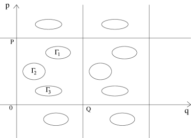
FIG. 2.: The energy level $E$ in the phase space.

Our purpose is now to establish under which conditions (shape and locations of the trajectories $\Gamma_{i}$) degeneracies in the spectrum of $\hat{H}$ may occur semi-classically near the energy $E$. More precisely, we will describe the generic degeneracy lines in the space $\gamma$.

A The tunnelling interaction matrix.

In this section, we construct a basis of $H_{N}(\theta_{1},\theta_{2})$ and describe the asymptotic of the matrix of the Hamiltonian $H$ in this basis. To have a more precise picture of these asymptotics, we will make assumptions on the respective decays of interaction terms.

For a first reading, one can skip this section and refer to the results mentionned in proposition 8.

Using the ellipticity of $\hat{H}-E$ outside the classical region $H(q,p)=E$, it is easy to prove that the eigenfunctions are of order $O(h^{N})$ for all $N\in I\!\!N$ (noted $O(h^{\infty})$) outside the classical region. This property is in fact sufficient to construct a basis of $H_{N}(\theta_{1},\theta_{2})$.

It is easy to modify the Hamiltonian $H$ in a new hamiltonian $\tilde{H}_{1}$ such that:

• the energy shell $E$ of $\tilde{H}_{1}$ is $\Gamma_{1}$,

• $H=\tilde{H}_{1}$ outside the shaded region, see figure 3, p.3.

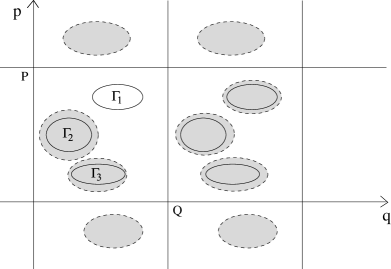
FIG. 3.: Modification of $H$.

Let $|1>$ be an eigenfunction of $\tilde{H}_{1}$ corresponding to an eigenvalue $\tilde{E}_{1}(h)$ such that $\tilde{E}_{1}(h)\rightarrow E$ as $h\rightarrow 0$. Then $(\hat{H}-\tilde{E}_{1})|1>=(\hat{H}-\tilde{H}_{1})|1>$. In the last expression, the operator is microlocally supported in the shaded region where $|1>$ is not. Hence:

$\displaystyle(\hat{H}-\tilde{E}_{1})|1>=O(h^{\infty})$

The same construction applies for the trajectories $\Gamma_{2}$ and $\Gamma_{3}$ and we get the functions $|2>$ and $|3>$ microlocally supported on $\Gamma_{2}$ and $\Gamma_{3}$ respectively . In the sequel, we will denote by $r$ the greatest of the quantities $|(\hat{H}-\tilde{E}_{i})|i>|$ ($i=1,2,3$).

¿From $|1>$, $|2>$ and $|3>$ we construct Floquet-periodic quasimodes:

$$|\varphi_{i}>=P(\theta_{1},\theta_{2})|i>\mbox{ for }i=1,2,3$$ (17)

where $P(\theta_{1},\theta_{2})$ is the operator from $L^{2}(R)$ to $H_{N}(\theta_{1},\theta_{2})$ which makes a given state Floquet-periodic:

$$P(\theta_{1},\theta_{2}):=\sum_{n_{1},n_{2}\in Z^{2}}\exp(-in_{1}\theta_{1}-in_{2}\theta_{2})T_{Q}^{n_{1}}T_{P}^{n_{2}}$$ (18)

Figure 4 p.4 and 5 p.5 shows the microlocal support of $|1>$ and $|\varphi_{1}>$.

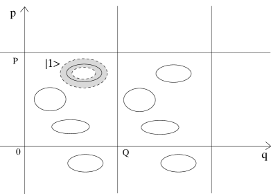
FIG. 4.: Microlocal support of the states $|1>$ in the phase space.

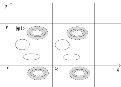
FIG. 5.: Microlocal support of the state $|\varphi_{1}>$ in the phase space.

Suppose that we are in the resonance situation: $\tilde{E}_{i}(\hbar)-\tilde{E}_{j}(\hbar)=o(\hbar)$ for $i,j=1,2,3$. Then for $\varepsilon>0$ sufficiently small the spectrum of $\hat{H}$ in the interval $I=[\tilde{E}_{1}(\hbar)-\varepsilon\hbar,\tilde{E}_{1}(\hbar)+\varepsilon\hbar]$ is made of 3 eigenvalues $E_{1}(\hbar)$, $E_{2}(\hbar)$ and $E_{3}(\hbar)$, and if we denote by $\Pi_{I}(\theta)$ the corresponding spectral projector of $H_{N}(\theta)$, the spectral space is spanned by:

$\displaystyle|\psi_{i}>=\Pi_{I}(\theta)|\varphi_{i}>,\quad i=1,2,3.$

Note that for a critical trajectory the width of the interval must be $\varepsilon\hbar/|\ln\hbar|$.

Let $C$ be the circle of center $\tilde{E}_{1}(\hbar)$ and radius $\varepsilon\hbar$ in the complex plane. We represent $\Pi_{I}$ and identity as:

$\displaystyle\Pi_{I}=\frac{1}{2\pi i}\int_{C}(\hat{H}-z)^{-1}\ dz,\quad Id=\frac{1}{2\pi i}\int_{C}(\tilde{E}_{1}-z)^{-1}\ dz\quad Id,$

and get:

$$|\psi_{i}>-|\varphi_{i}> = \frac{1}{2\pi i}\int_{C}[(\hat{H}-z)^{-1}-(\tilde{E}_{1}-z)^{-1}]|\varphi_{i}>\ dz$$

$$= \frac{1}{2\pi i}\int_{C}-(\hat{H}-z)^{-1}(\tilde{E}_{1}-z)^{-1}(\hat{H}-\tilde{E}_{1})|\varphi_{i}>\ dz$$

$$= O(r/h^{2})(=O(h^{\infty}))$$

since $||(\hat{H}-z)^{-1}||<K/(\varepsilon\hbar)$ and $|\tilde{E}_{1}-z|^{-1}<K/(\varepsilon\hbar)$ for $z\in C$. In the following text, we replace $r/h^{2}$ by $r$, the new $r$ function has decay properties similar to the original one ($r=O(h^{\infty})$ and is probably exponentially decaying).

Hence $|\psi_{i}>$ is microlocalized on $\Gamma_{i}$ like $|\varphi_{i}>$.

The next step is to get an orthonormalized basis from the $(|\psi_{i}>)_{i}$. Let

$$n_{ij}=<\psi_{j}|\psi_{i}>,\quad N=(n_{ij})_{i,j}$$ (19)

Since $N$ is positive hermitian, there exists a unique positive hermitian matrix $B$ such that:

$$B^{-2}=N$$ (20)

Let $B=(\beta_{ij})_{i,j}$ (with $\beta_{ij}=\overline{\beta_{ji}}$) and:

$$|e_{i}>=\sum_{j}\beta_{ij}|\psi_{j}>$$ (21)

We claim that the family $|e_{i}>$ is orthonormal. Indeed:

$$<e_{i}|e_{j}> = \sum_{k,l}\overline{\beta_{ik}}\beta_{jl}<\psi_{k}|\psi_{l}>$$

$$= \sum\beta_{jl}n_{lk}\beta_{ki}$$

$$= (BNB)_{ji}$$

$$= (Id)_{ji}$$

The tunnelling interacting matrix is the $3\times 3$ Hermitian matrix:

$$A=(<e_{i}|\hat{H}|e_{j}>)_{ij}$$ (22)

The eigenvalues of $A$ are exactly the eigenvalues of $\hat{H}$ which belong to the $I$ interval.

We will now compute the semi-classical asymptotics of $a_{ij}$. Let:

$$G=(<\psi_{i}|\hat{H}|\psi_{j}>)_{i,j=1,2,3}$$ (23)

¿From Eq. (21), we get:

$$A=\overline{B}G\overline{B}$$ (24)

hence we want to compute asymptotics of $B$ and $G$.

First we remark that in Eq.(19), we can replace $|\psi>$ by $|\varphi>$, since by Pythagoras theorem:

$$<\varphi_{i}|\varphi_{j}>=<\psi_{i}|\psi_{j}>+<\varphi_{i}-\psi_{i}|\varphi_{j}-\psi_{j}>=<\psi_{i}|\psi_{j}>+O(r^{2})$$ (25)

Since $\hat{H}$ commutes with $\Pi_{I}$, we get by the same method:

$\displaystyle<\varphi_{i}|\hat{H}|\varphi_{j}>=<\psi_{i}|\hat{H}|\psi_{j}>+<\varphi_{i}-\psi_{i}|\hat{H}|\varphi_{j}-\psi_{j}>=<\psi_{i}|\hat{H}|\psi_{j}>+O(r^{2})$

We have

$\displaystyle<\varphi_{i}|\varphi_{j}>=\delta_{ij}+O(r)$

Hence:

$$N=Id+O(r),\quad B=Id+O(r)$$ (26)

Now, we want to expand the functions $|\varphi_{i}>$ using (17) and (18) and evaluate the scalar products. ¿From Eq.(23) and (17), we get:

$$<\psi_{1}|\hat{H}|\psi_{1}>=<1|\hat{H}|1>+2\sum_{\vec{n}\in D}Re\left(\exp(-i\vec{n}\vec{\theta})<1|\hat{H}|1_{\vec{n}}>\right)$$ (27)

where:

• $\vec{n}=(n_{1},n_{2})$, $\vec{\theta}=(\theta_{1},\theta_{2})$,

• $D=\{(Z\!\!\!Z\times I\!\!N)\setminus(-I\!\!N\times\{0\})\}$ is the half plan of $\vec{n}$,

• $|1_{\vec{n}}>=T_{Q}^{n_{1}}T_{P}^{n_{2}}|1>$ is a quasi mode concentrated on the translated trajectory $(\Gamma_{1})_{n_{1},n_{2}}$ in the $(n_{1},n_{2})$ cell of the phase space.

The first term of (27) is $\tilde{E}_{1}+O(r^{2})$. The term $<1|\hat{H}|1_{\vec{n}}>$ is of order $O(r)$ because it corresponds to the tunnelling interaction between the quasimode $|1>$ localized in cell $(0,0)$ and the quasi mode $|1_{\vec{n}}>$ localized in the cell $(n_{1},n_{2})\neq(0,0)$ (we may need to modify the function $r$ to get this decay: $r$ denotes the strongest tunneling interaction between two components of the energy shell). Hence:

$\displaystyle<\psi_{1}|\hat{H}|\psi_{1}>=\tilde{E}_{1}+O(r)$

Similar asymptotics hold for the other diagonal terms.

A non-diagonal term of $G$ is e.g.:

$$<\psi_{1}|\hat{H}|\psi_{2}>=\sum_{\vec{n}\in Z\!\!\!Z^{2}}\exp(-i\vec{n}\vec{\theta})<1|\hat{H}|2_{\vec{n}}>$$ (28)

And there is generically only one leading term due to the strongest tunnelling interaction between $|1>$ and $|2_{\vec{n}_{12}}>$ (located in the cell $\vec{n}_{12}$: $\vec{n}_{12}$ may be for example $(0,0)$ or $(0,\pm 1)$ or $(\pm 1,0)$), of strength

$\displaystyle<1|\hat{H}|2_{\vec{n}_{12}}>=m_{12}\exp(i\varphi_{12})$

where $m_{12}>0$ is $O(r)$. This gives:

$\displaystyle<\psi_{1}|\hat{H}|\psi_{2}>\equiv m_{12}\exp(i(\varphi_{12}-\vec{n}_{12}\vec{\theta}))$

and similar expressions for others non-diagonal terms. Hence all non-diagonal terms are $O(r)$. If we denote by $\tilde{r}$ the second strongest tunneling interaction, we have

$\displaystyle<\psi_{1}|\hat{H}|\psi_{2}>=m_{12}\exp(i(\varphi_{12}-n_{12}\theta))+O(\tilde{r})$

We assume of course that $\tilde{r}=O(h^{\infty})r$.

¿From $A=\overline{B}G\overline{B}$, $B=N^{-1/2}$ and $N=Id+O(r)$, we get for the diagonal terms of $A$:

$\displaystyle a_{ii}=\tilde{E}_{i}+O(r)$

and for the non-diagonal terms:

$$a_{ij}=m_{ij}\exp(i(\varphi_{ij}-\vec{n}_{ij}\vec{\theta}))+O(\tilde{r})$$ (29)

To get a more accurate asymptotic of the diagonal terms, we will now study the shifted interaction matrix:

$\displaystyle<e_{i}|\hat{H}-\tilde{E}_{3}|e_{j}>=\overline{B}(G-\tilde{E}_{3}N)\overline{B}$

We have $G-\tilde{E}_{3}N=(<\psi_{i}|\hat{H}-\tilde{E}_{3}|\psi_{j}>)_{ij}$. For the non-diagonal terms, we get similar asymptotics as above (29) with new constants. For simplicity, we will however keep the same notations, since the decays remain of the same order and the phases were not explicit. For the diagonal terms, we get by the same method:

$$(<\psi_{i}|H-\tilde{E}_{3}|\psi_{i}>)=\tilde{E}_{i}-\tilde{E}_{3}+m_{ii}\cos(\varphi_{ii}-n_{ii}\theta)+...$$ (30)

Since $B=I$ modulo $O(r)$ and $G-\tilde{E}_{3}N$ is of order $O(r)$, the shifted interaction matrix is $G-\tilde{E}_{3}N$ modulo an error of order $O(\tilde{r})$.

In this section we have used he fact that the tunnelling interaction gives terms of order $r=O(h^{\infty})$. In fact the reader may replace $O(h^{\infty})$ by $O(e^{-S/h})$ which is conjectured to be the right decay order, where $S$ is similar to the Agmon distance between two trajectories (as in the Schrödinger case $H=p^{2}/2+V(x)$). See [21], [23] for partial results in this direction).

We summarize the results of this section:

Proposition 8

Let $H$ be a Hamiltonian and $E$ an energy such that the energy shell $H=E$ is made of three contractible connected components. Let $|1>$, $|2>$, $|3>$ be the quasimodes of $\hat{H}$ localized near one of the three classical trajectories corresponding to eigenvalues $\tilde{E}_{1}(\hbar)\rightarrow E$, $\tilde{E}_{2}(\hbar)\rightarrow E$, $\tilde{E}_{3}(\hbar)\rightarrow E$ Suppose that $\tilde{E}_{i}(\hbar)-\tilde{E}_{j}(\hbar)=o(\hbar)$. Then for $\varepsilon>0$ and $\hbar>0$ sufficently small, the spectrum of $\hat{H}$ acting on $H_{N}(\theta_{1},\theta_{2})$ in the interval $[\tilde{E}_{3}(\hbar)-\varepsilon\hbar,\tilde{E}_{3}(\hbar)+\varepsilon\hbar]$ is made of three eigenvalues.

We have constructed an orthonormal basis $|e_{i}>$ spanning the corresponding 3-dimensionnal vector space. Let $r$ be a majorant of the largest tunneling interaction between two different trajectories, and $\tilde{r}$ be a majorant of the second largest tunneling interaction between two wells ($r=O(\hbar^{\infty})$ and $\tilde{r}=O(h^{\infty}r)$. More precisely, we choose $i$ and $j$ in$[1,3]$, we look at the second strongest interaction between trajectory $i$ and translated of the trajectories $j$, excluding the 0 translation if $i=j$. $r$ and $\tilde{r}$ are conjectured to be exponentially decreasing with respect to $r$). Then the matrix of $\hat{H}$ in the basis $|e_{i}>$ has the following asymptotic:

• The non-diagonal terms are $O(r)$, more precisely:

  
  

  $\displaystyle a_{ij}=m_{ij}\exp{i(\varphi_{ij}-\vec{n}_{ij}.\vec{\theta})}+O(\tilde{r}),\quad m_{ij}=O(r)$

• The diagonal terms are given by:

  
  

  $\displaystyle a_{ii}=\tilde{E}_{i}+m_{ii}\cos(\varphi_{ii}-\vec{n}_{ii}.\vec{\theta})+O(\tilde{r})$

If we look at the dependency of the interaction matrix with respect to the external parameters $\gamma$, it is easy to prove that:

$\displaystyle d_{\gamma}a_{ij}=(d_{\gamma}\tilde{E}_{i})\delta_{ij}+O(r)$

where $d_{\gamma}$ denote the differential. The first term is dominant, since the variation of $\tilde{E}_{i}$ is of order $\hbar$ (or $\hbar/|\ln\hbar|$ for a critical trajectory).

Since we are interested in eigenvalue degeneracies, we may substract $\tilde{E}_{1}.I_{3}$ to the interaction matrix, hence the variation of the shifted interaction matrix with respect to $\gamma$ is described by the variation of $\tilde{E}_{1}-\tilde{E}_{3}$ and $\tilde{E}_{2}-\tilde{E}_{3}$ with respect to $\gamma$ up to an error of order $r$. Hence, we will reduce our parameter space to two parameters $\gamma_{1}$ and $\gamma_{2}$, and we justify in appendix B that they can be chosen as:

$$\gamma_{1} = (\tilde{E}_{1}-\tilde{E}_{3})/\hbar$$ (31)

$$\gamma_{2} = (\tilde{E}_{2}-\tilde{E}_{3})/\hbar$$ (32)

(replace $\hbar$ by $\hbar/|\ln\hbar|$ for a critical trajectory).

Moreover, since the error is of order $O(r)$, the degeneracy lines in the parameter space will be of $O(\hbar^{\infty})$ size (and conjectured to be of exponentially small size). We will come back to this point more precisely in section VI C.

B Model of a 3$\times$3 interaction matrix, and computation of its Chern indices.

This paragraph is self-contained. From the previous paragraph, we have to consider a continuous mapping on the torus $T_{\theta}=[0,2\pi[^{2}$ into the 3$\times$3 Hermitian matrices:

$\displaystyle{\cal A}:(\theta_{1},\theta_{2})\in T_{\theta}\rightarrow A(\theta_{1},\theta_{2})=(a_{i,j})_{i,j=1,2,3}$

where the diagonal terms are:

$$a_{ii}=\tilde{E_{i}}+m_{ii}\cos(\varphi_{ii}-\vec{n}_{ii}\vec{\theta})\hskip 28.45274pti=1,2,3$$ (33)

and the non-diagonal terms are

$$a_{ij}=m_{ij}\exp i(\varphi_{ij}-\vec{n}_{ij}\vec{\theta})\hskip 28.45274pti<j=1,2,3$$ (34)

with $\vec{n}_{ij}=(n_{1(ij)},n_{2(ij)})\in Z^{2}$ and $\vec{\theta}=(\theta_{1},\theta_{2})$. We consider $(m_{ij},\varphi_{ij},\vec{n}_{ij})_{i,j=1,2,3}$ as fixed. We will study only the dependance of $\cal A$ with the parameters $(\tilde{E_{1}},\tilde{E_{2}},\tilde{E_{3}})$.

We recall that $(m_{ij},\varphi_{ij},\vec{n}_{ij})$ refer to the tunnelling interaction between the three trajectories $(\Gamma_{i})_{i},i=1,2,3$ as sketched in figure (6), and that $\tilde{E_{i}}$ is the energy of the quasimodes on trajectory $\Gamma_{i}$.

If no degeneracy occurs in the spectrum of $A(\theta_{1},\theta_{2})$ (for all $\vec{\theta}=(\theta_{1},\theta_{2})\in T_{\theta}$), each eigenvector family has a well defined Chern index. Precisely, each eigenvector family $(|\psi_{n}(\vec{\theta})>)_{\vec{\theta}}$ for $n=1,2,3$ is a submanifold of the projective space $P(I\!\!\!\!C^{3})$, homeomorphic to $T_{\theta}$. The complex line bundle structure of $P(I\!\!\!\!C^{3})$ induces a complex line bundle over this submanifold whose topology is characterized by its Chern index. For specific values of the parameters (codimension 1 in the space of $(\tilde{E_{i}})_{i}$) degeneracies occur and this causes a change of the Chern index. In this paragraph we will compute these Chern indices and the locus of the degeneracies in the space of $(\tilde{E_{i}})_{i}$ for each family of eigenvector $(|\psi_{n}(\vec{\theta})>)_{\vec{\theta}}$ for $n=1,2,3$. First we remark that substracting the diagonal matrix $\tilde{E_{3}}Id$ to $A$ does not change its eigenvectors, so the only non-trivial external parameters are:

$$\gamma_{1} = (\tilde{E}_{1}-\tilde{E}_{3})/\hbar$$ (35)

$$\gamma_{2} = (\tilde{E}_{2}-\tilde{E}_{3})/\hbar$$ (36)

The locus of the degeneracies we are looking for are lines in the space $(\gamma_{1},\gamma_{2})$.

A general property of $3\times 3$ Hermitian matrices, mentioned in the appendix A is that a degeneracy occurs for the matrix $A$ if and only if:

$$\Im(a_{12}a_{23}a_{31}) = 0$$ (37)

$$a_{11}-a_{22}+\frac{a_{12}a_{23}}{a_{13}}-\frac{a_{21}a_{13}}{a_{23}} = 0$$ (38)

$$a_{22}-a_{33}+\frac{a_{13}a_{32}}{a_{12}}-\frac{a_{12}a_{23}}{a_{13}} = 0$$ (39)

$\Im$ stands for imaginary part. Moreover, the degeneracy is between levels $n=1,2$ (respect. $n=2,3$) if $\Re(a_{12}a_{23}a_{32})>0$ (respect $<0$).

The first equation can be written:

$$\Theta=\arg(a_{12}a_{23}a_{31})=\varphi_{12}+\varphi_{23}+\varphi_{31}-(\vec{n}_{12}+\vec{n}_{23}+\vec{n}_{31})\vec{\theta}\equiv 0\qquad[\pi]$$ (40)

The phase $\Theta$ can be seen as the total tunnelling phase for the cycle of trajectories $(\Gamma_{1},\Gamma_{2},\Gamma_{3})$. We want to find solutions in $\vec{\theta}$ of this equation for fixed values of $\varphi_{ij},\vec{n}_{ij}$. For that purpose, we assume that $(\vec{n}_{12}+\vec{n}_{23}+\vec{n}_{31})\neq 0$. This is a generic assumption. This means that the cycle of trajectories $(\Gamma_{1},\Gamma_{2},\Gamma_{3})$ is not contractible on the torus $T_{qp}$.

To simplify notations, we will assume that $\vec{n}_{12}=\vec{n}_{23}=0$, $\vec{n}_{31}=(0,1)$ and $\vec{n}_{ii}=(1,0)$. This corresponds to the tunnelling interactions sketched with dashed lines in figure (6). For the tunnelling problem considered in this paper, we think (without proof) that this case is the general one after a suitable lattice transformation in $SL(2,Z)$. But for the self-contained problem of this paragraph, the general case is solved in the appendix C.

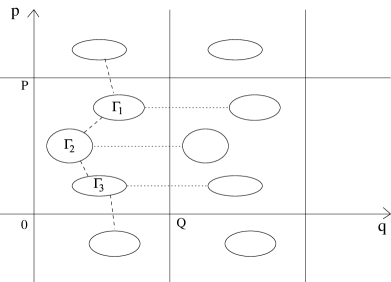
FIG. 6.: Example of tunnelling interaction. $\vec{n}_{12}=\vec{n}_{23}=0$, $\vec{n}_{31}=(0,1)$ and $\vec{n}_{11}=\vec{n}_{22}=\vec{n}_{33}=(1,0)$.

Eq. (40) has then two solutions $\theta_{2}\equiv\varphi_{12}+\varphi_{23}+\varphi_{31}\qquad[\pi].$

Let

$\displaystyle s=\exp(i\Theta)=\pm 1.$

The two-last equations of Eq. (37) give:

$$\tilde{E}_{1}-\tilde{E}_{3}=sm_{13}\left(\frac{m_{12}}{m_{23}}-\frac{m_{23}}{m_{12}}\right)+m_{33}\cos(\varphi_{33}-\theta_{1})-m_{11}\cos(\varphi_{11}-\theta_{1})$$ (41)

and similarly for $\tilde{E}_{2}-\tilde{E}_{3}$.

Let us remark that:

$$A\cos(\theta_{1}-\alpha)-B\cos(\theta_{1}-\beta) = (A\cos\alpha-B\cos\beta)\cos\theta_{1}+(A\sin\alpha-B\sin\beta)\sin\theta_{1}$$

$$= D\cos(\theta_{1}-\eta)$$

where:

$$D = \sqrt{A^{2}+B^{2}-2AB\cos(\alpha-\beta)},$$ (42)

$$(\cos\eta,\sin\eta) = \left(\frac{A\cos\alpha-B\cos\beta}{D},\frac{A\sin\alpha-B\sin\beta}{D}\right)$$ (43)

So we put:

$$K_{1} = \sqrt{m_{11}^{2}+m_{33}^{2}-2m_{11}m_{33}\cos\varphi_{1}}$$ (44)

$$K_{2} = \sqrt{m_{22}^{2}+m_{33}^{2}-2m_{22}m_{33}\cos\varphi_{2}}$$ (45)

where:

$\displaystyle\varphi_{i}=\varphi_{ii}-\varphi_{33}$

and define:

$\displaystyle Y_{1}=m_{13}\left(\frac{m_{12}}{m_{23}}-\frac{m_{23}}{m_{12}}\right)\quad Y_{2}=m_{23}\left(\frac{m_{12}}{m_{13}}-\frac{m_{13}}{m_{12}}\right)$

From (41) and (35), the degeneracy lines in the space $(\gamma_{1},\gamma_{2})$ are the following $t\in I\!\!R$ parametrized curves ($s=\pm 1$):

$$\gamma_{1}(t) = (K_{1}\cos(t-\eta)-sY_{1})/\hbar$$ (46)

$$\gamma_{2}(t) = (K_{2}\cos(t)-sY_{2})/\hbar$$ (47)

where $s=\pm 1$, $t=\theta_{1}-\eta_{2}$, $\eta=\eta_{3}-\eta_{2}$ and the angles $\eta_{2}$ and $\eta_{3}$ may be computed using (42).
As $t$ describes $[0,2\pi]$, $(\gamma_{1}(t),\gamma_{2}(t))$ describes two translated ellipses of axes parallel to $\gamma_{1}=\pm\gamma_{2}$, one for each $s\in\{-1,1\}$. $s=1$ (respect. $s=-1$) gives the degeneracy line between levels $n=1,2$ (respect. levels $n=2,3$). See figure (7). These two ellipses may intersect, but they don’t really intersect in the whole space $(\theta_{1},\theta_{2},\gamma_{1},\gamma_{2})$ because they correspond to two different values of $\theta_{2}$.

Outside the ellipses, the Chern indices are zero. This is because, when $\gamma_{1},\gamma_{2}\rightarrow\infty$ the $A$ matrix goes to a diagonal matrix with trivial eigenvectors. Crossing a degeneracy line changes a Chern index change by $\pm 1$. It can be shown that the value $\pm 1$ is related to the orientation relatively to the orientation of the parametrized ellipse. From this, we deduce the values of the Chern indices in figure (7).

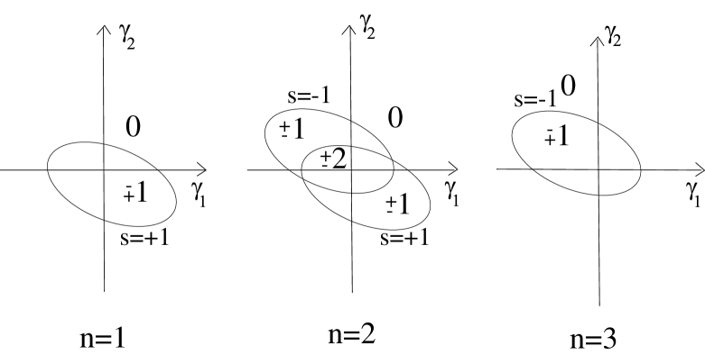
FIG. 7.: Degeneracies lines and value of Chern indices from Eq.(46).

C The degeneracy lines are ellipses.

We are now ready to present the final result. Consider a generic two-dimensional submanifold of the manifold of classical Hamiltonian $H_{\gamma}$ ($\gamma$ are coordinates on this manifold, and can be viewed as external parameters of the Hamiltonian). We have obtained that in this space, degeneracy lines are two ellipses (one for each pair of levels $(1,2)$ and $(2,3)$).

Note that it make sense to state that the shape of the curves are ellipse even if the $H_{\gamma}$-space is a manifold. This is because the ellipse are exponentially small, and thus live in the tangent space.

More precisely, there exist a coordinate system $(\gamma_{1},\gamma_{2})$ (i.e. a special parametrization of the Hamiltonian) for which the two ellipses are given by Eq. (46). The width of the ellipses are given by the coefficients $K_{1},K_{2}$, whereas the position of the centers are given by coefficients $sY_{1},sY_{2}$, $s=\pm 1$.

It is obvious from Eq. (44) that $K_{1},K_{2}$ are exponentially small in the semi-classical limit. But this is true also for $Y_{1},Y_{2}$. This is shown at the beginning of the appendix (B).

We have then two different generic situations in the semi-classical limit:

1. case: the non-diagonal terms $Y_{1},Y_{2}$ are exponentially small with respect to the diagonal terms $K_{1},K_{2}$. The two ellipses are identical, see figure 8 p. 8. At the origin, the three bands of energy will have Chern indices of $(\mp 1,\pm 2,\mp 1)$. Outside the ellipse, the Chern indices are $(0,0,0)$. Note that in the $(\gamma_{1},\gamma_{2})$ parameter space, the ellipse are exponentially small and exponentially flat because $K_{1}$ is exponentially small compare to $K_{2}$ (or the inverse).

   

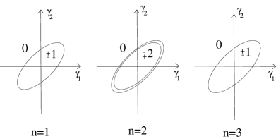
   FIG. 8.: Degeneracies lines and value of Chern indices in case 1.

2. case: the diagonal terms $K_{1},K_{2}$ are exponentially small with respect to the non-diagonal ones $Y_{1},Y_{2}$. See figure 9, p. 9. At the scale $Y_{i}$ of the distance between the two center, the degeneracy lines collapse to 2 single points as $\hbar$ tends to 0. Individually these lines are still elliptical with respect to their own scale $K_{i}$.

   

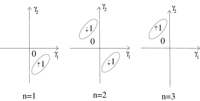
   FIG. 9.: Degeneracies lines and value of Chern indices in case 2.

The non-generic intermediate case occurs when the diagonal terms $K_{i}$ and non-diagonal terms $Y_{i}$ are of the same order. Hence the degeneracies are two ellipses ($s=\pm 1$) with symmetric centers. These two ellipses may intersect. Corrections to the leading behaviour in the semi-classical limit can modify the shape and sizes of the ellipses, see the numerical section.

We now discuss the special translation-symmetric case corresponding to the first calculation of Chern indices done by Thouless and al. [27]. For example, take $H(q,p)$ from Eq. (49) with $b=\gamma_{1}=\gamma_{2}=0$. See also remark 1. We construct $|2>={\hat{T}}_{P/3}|1>$ and $|3>={\hat{T}}_{P/3}|2>$ by translation by $P/3$ in the momentum direction. Applying the relation $T_{P/3}T_{Q}=e^{2i\pi N/3}T_{Q}T_{P/3}$ we get:

$$\varphi_{2}=\varphi_{1}/2=-\varphi_{1}=-\frac{2\pi N}{3}$$ (48)

Since the non-diagonal $m_{ij}$ are equal, so we are in the first case (double ellipse centered at the origin of figure 8). Assuming that $3$ doesn’t divide $N$ then we get $K_{1}=K_{2}$ and the precise shape of the ellipse:

$\displaystyle\gamma_{1}=\frac{K}{\hbar}\cos(t),\quad\gamma_{2}=\frac{K}{\hbar}\cos(t\pm\frac{2\pi}{3})$

We conclude that we get an ellipse of axes $\gamma_{1}=\pm\gamma_{2}$ and excentricity $\sqrt{2/3}$.

Remark 9

We want to stress that all the results obtained in this section are valid modulo error terms of order $O(r^{2})$, where $r=O(h^{\infty})$ is the greatest tunnelling interaction between two wells. If one of the previous contributions $m_{ij}$ between two other wells is smaller than $r^{2}$, it is not significant. For example, if we consider an Hamiltonian where wells 2 and 3 are very closed compared to well 1, our method must be modified, although we think that our results Eq. (46) are still qualitatively correct. In this situation, a more convenient approach is to first treat the cluster of wells 2 and 3 and finally consider the interaction between the cluster and well 1. By this approach, we obtain results similar to those described in [10] for the 2-wells problem.

VII Numerical illustration

More precise informations on how to perform the numerical simulation, and a software will be available on the web address: http://www-fourier.ujf-grenoble.fr/~parisse or http://lpm2c.polycnrs-gre.fr/~faure

We take the following Hamiltonian on the torus, parametrized by $\gamma_{1}$ and $\gamma_{2}$:

$$H(q,p)= \cos(2\pi\frac{q}{Q})+\cos(6\pi\frac{p}{P})$$ (49)

$$+4b\sin(2\pi\frac{q}{Q})\cos(2\pi\frac{p}{P})$$ (50)

$$+((\gamma_{1}-\gamma_{2})\cos(2\pi\frac{p}{P})+((-\gamma_{1}-\gamma_{2})\sin(2\pi\frac{p}{P})$$ (51)

The two terms in the first line are the main part of the Hamiltonian. They create three symmetric wells in the $p$ direction in the lower part of the energy spectrum, see figure (10). The second line breaks this symmetry, by moving the second well on the left when $b$ increases. $b$ can be seen as a perturbation from the translational symmetric case. The coefficients $\gamma_{1}$ and $\gamma_{2}$ in the third line change the depth of wells 1 and 3 respectively. We therefore expect them to act directely on $(\tilde{E}_{1}-\tilde{E}_{2})$ and $(\tilde{E}_{3}-\tilde{E}_{2})$ respectively, such that (B1) will be satisfied. In figure (10) it seems clear that the main tunnelling interactions between the wells are those sketched in figure (6) as assumed for the calculations of the previous section.

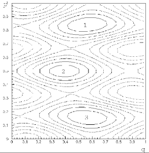
FIG. 10.: Contour levels of Hamiltonian (49), with $b=0.2$ and $\gamma_{1}=-\gamma_{2}=-0.1$

For the numerical calculations, the Hamiltonian (49) has been diagonalized and formula (13) has been used to obtain the Chern indices $C_{n}$. Maps of the Chern indices have been numerically obtained by varying parameters $\gamma_{1}$ and $\gamma_{2}$.
For $N=17$ the values of the Chern indices for the first three energy bands $n=1,2,3$ are shown in figure 11.

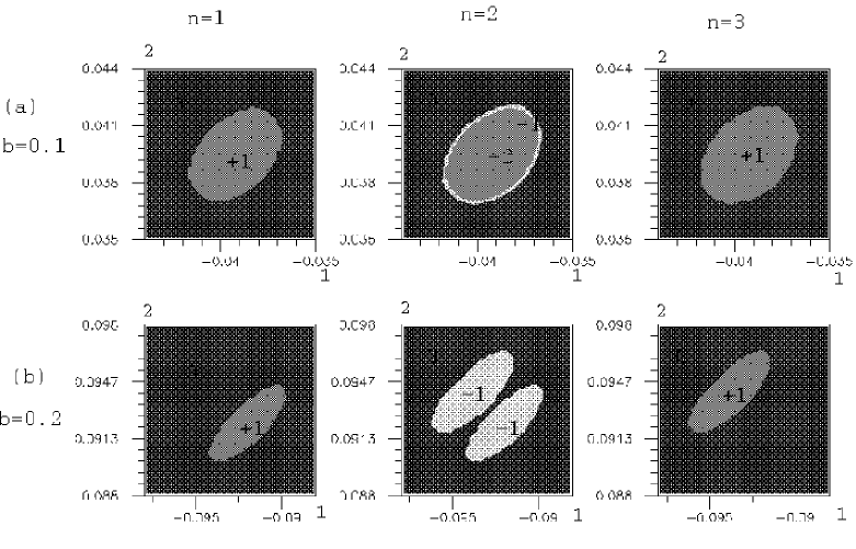
FIG. 11.: Chern indices for the first three bands $n=1,2,3$, for $N=17$. Case (a): The strength of the perturbation is $b=0.1$. Case (b): The strength of the perturbation is $b=0.2$.

In case (a), the strength of the perturbation is $b=0.1$. The two ellipses are degenerated. This is the generic situation depicted in figure (8), and the same generic situation as for the translation-symmetric case with $b=0$, treated in the previous section. This means that the parameter $b=0.1$ is small enough to stay in the same generic ensemble.
In case (b), the strength of the perturbation is $b=0.2$. The two ellipses are separated, as in the second generic situation, sketched in figure (9).
In case (a) and (b), the two ellipses have the same shape, in agreement with the semi-classical results of the previous section.
Figure 12 shows results for a lower value of $N$, $N=11$, and for strengths $b=0.2$ and $b=0.25$. Here, the generic situations expected in the semi-classical limit $N\rightarrow+\infty$ are less visible. There are still elliptical curves (from a topological point of view), but their position and shapes are affected by non-leading corrections with respect to $N\rightarrow+\infty$.

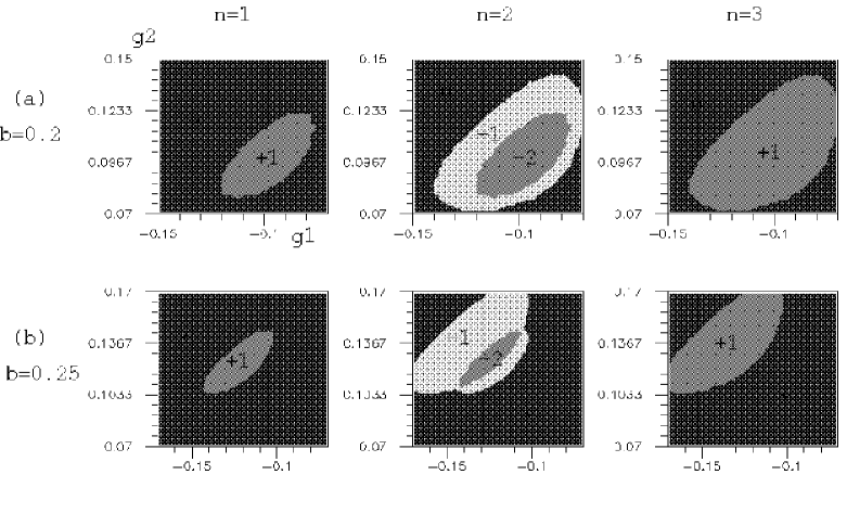
FIG. 12.: Chern indices for the first three bands $n=1,2,3$, for $N=11$. Case (a): The strength of the perturbation is $b=0.2$. Case (b): The strength of the perturbation is $b=0.25$.

VIII Conclusion

In this paper, we have shown in which conditions a non-zero Quantum Hall conductivity can occur in the framework of the Harper model, and for the tunnelling between three trajectories in a periodic cell. In this framework, the Hall conductivity is proportional to the topological Chern index. These results were derived semi-classically and give at the same time a description of degeneracies in the spectrum.

Currently, one tries to observe experimental signatures of the Harper spectrum (Landau level substructures) in lateral superlattices with periods of about $100nm$ on GaAs-AlGaAs heterojunctions [12, 24]. Our results could therefore have some experimental importance in the future.

The main mathematical gap in this work is that we do not have results about microlocal tunnelling effect (like those obtained by Helffer and Sjöstrand [13] in the Schrödinger case). The main ideas to solve these difficulties are currently majorations of the wave function (A.Martinez [21]), complex paths (estimations of the tunnelling effect by Wilkinson [31, 32]), or normal forms (S.Nakamura [23]), but the authors are not aware of a general rigorous result.

Some other related problems could be investigated in the future like:

• numerical localization in the $\gamma$-space of the ellipsis (this requires numeric estimations of the tunnelling effect),

• generic interaction between $N$ bands ($N$-wells tunnelling effect) by a recursive clustering approach,

• the tunnelling effect between non-contractible classical trajectories

Acknowledgments

We would like to thank P. Leboeuf for giving the initial impulse of this work and Y. Colin de Verdière for his constant interest, his patient relecture of this work and the subsequent remarks he made.

A Eigenvalue degeneracies in 3$\times$3 hermitian matrices.

In the text, we use the following result of linear algebra that we have not found in the literature:

Theorem 10

Let $A$ be a $3\times 3$ Hermitian matrix:

$\displaystyle A=\left(\begin{array}[]{ccc}a&\delta&\gamma\\ \bar{\delta}&b&\varepsilon\\ \bar{\gamma}&\bar{\varepsilon}&c\end{array}\right)$

where $a,b,c$ are real numbers and $\gamma,\delta,\varepsilon$ are non-zero complex numbers.

Then $A$ has a eigenvalue $\lambda$ with multiplicity at least $2$ if and only if:

$\displaystyle a-\frac{\bar{\delta}\gamma}{\varepsilon}=b-\frac{\delta\varepsilon}{\gamma}=c-\frac{\gamma\bar{\varepsilon}}{\delta}=\lambda\in R$

(this is a system of $3$ real equations). The third eigenvalue is $\lambda=tr(A)-2\lambda$ and the spectrum is $(\lambda,\lambda,\lambda^{\prime})$ with $\lambda^{\prime}>\lambda$ iff $\Re(\delta\varepsilon\bar{\gamma})>0$.

Proof
Let us recall that a hermitian matrix has real eigenvalues and is diagonalizable. Then $A$ has an eigenvalue $\lambda$ with multiplicity 2 or 3 if and only if its minimal polynomial has degree $2$ or $1.$ The matrix $A^{2}$ is then a linear combination of $I$ and $A$. We have:

$\displaystyle A^{2}=\left(\begin{array}[]{ccc}a^{2}+\left|\delta\right|^{2}+\left|\gamma\right|^{2}&(a+b)\delta+\gamma\bar{\varepsilon}&(a+c)\gamma+\delta\varepsilon\\ \ast&b^{2}+\left|\varepsilon\right|^{2}+\left|\delta\right|^{2}&(b+c)\varepsilon+\bar{\delta}\gamma\\ \ast&*&\left|\gamma\right|^{2}+\left|\varepsilon\right|^{2}+c^{2}\end{array}\right)$

where the stars denote the conjugate of the symmetric coefficients.

The other eigenvalue is $\lambda^{\prime}=tr(A)-2\lambda$, where $tr(A)$ denotes the trace of the matrix $A$. Therefore the minimal polynomial is:

$\displaystyle P(X)=(X-\lambda)(X-\mbox{tr}(A)+2\lambda)=X^{2}+(\lambda-\mbox{tr}(A))X-(2\lambda-\mbox{tr}(A))\lambda$

hence:

$\displaystyle A^{2}=(\mbox{tr}(A)-\lambda)A+\lambda(2\lambda-\mbox{tr}(A))$

Eventually we get the system:

$$\left\{\begin{array}[]{rcrcr}a^{2}+|\delta|^{2}+|\gamma|^{2}&=&(\mbox{tr}(A)-\lambda)a&+&\lambda(2\lambda-{tr}\,A)\\ b^{2}+|\delta|^{2}+|\varepsilon|^{2}&=&(\mbox{tr}(A)-\lambda)b&+&\lambda(2\lambda-{tr}\,A)\\ a^{2}+|\varepsilon|^{2}+|\gamma|^{2}&=&(\mbox{tr}(A)-\lambda)c&+&\lambda(2\lambda-{tr}\,A)\\ (a+b)\delta+\gamma\overline{\varepsilon}&=&(\mbox{tr}(A)-\lambda)\delta&&\\ (a+c)\gamma+\delta\varepsilon&=&(\mbox{tr}(A)-\lambda)\gamma&&\\ (b+c)\varepsilon+\overline{\delta}\gamma&=&(\mbox{tr}(A)-\lambda)\varepsilon&&\end{array}\right.$$ (A1)

But $\mbox{tr}(A)=a+b+c$, so the last three equations simplify to:

$\displaystyle\left\{\begin{array}[]{rcr}\gamma\overline{\varepsilon}&=&(c-\lambda)\delta\\ \delta\varepsilon&=&(b-\lambda)\gamma\\ \overline{\delta}\gamma&=&(a-\lambda)\varepsilon\end{array}\right.$

When $\delta$, $\gamma$, and $\varepsilon$ are non-zero, we verify that these three last equations imply the first three of system Eq. (A1). Indeed by multiplying two with two, we obtain:

$\displaystyle\left\{\begin{array}[]{rcr}|\varepsilon|^{2}&=&(b-\lambda)(c-\lambda)\\ |\delta|^{2}&=&(a-\lambda)(b-\lambda)\\ |\gamma|^{2}&=&(a-\lambda)(c-\lambda)\end{array}\right..$

The spectrum is $(\lambda,\lambda,\lambda^{\prime})$ iff $3\lambda<tr(A)$. This gives $\Re(\delta\varepsilon\bar{\gamma})>0$.

B Influence of the external parameters

In this appendix, we show that generically, only two external parameters $\gamma_{1},\gamma_{2}$ control degeneracies and the Chern indices, as in Eq. (31).

From the generic cyclic assumption made in section VI B, we have the property:

$\displaystyle\forall i\neq j,i\neq k,j\neq k,\quad m_{ij}m_{jk}\mbox{ is }O(h^{\infty})\mbox{ with respect to }m_{ik}$

In the analogous Schrödinger situation, this means that the triangular inequality is strict for the Agmon distance.

Remark 11

For the Agmon distance, the converse assumption is also generic (wells may be “shaded” by other wells). It is excluded here, because assuming that a well is shaded implies that the cycle of trajectories is contractible.

For example, if $H$ is symmetric under translation ${\hat{T}}_{P/3}$, we see that:

$\displaystyle m_{ij}m_{jk}/m_{ik}=m_{ij}=O(r)=O(h^{\infty})$

Then we get easily that $\tilde{E}_{i}-\tilde{E}_{j}$ must be $O(h^{\infty})$ in Eq. (41).

More precisely, we want to look at the $\gamma$-dependency of the two equations of (41). From the first equation, we define

$\displaystyle f_{1}(\gamma,\theta_{1})=\frac{1}{\hbar}\left((\tilde{E}_{1}-\tilde{E}_{3})-\left[sm_{13}\left(\frac{m_{12}}{m_{23}}-\frac{m_{23}}{m_{12}}\right)+m_{33}\cos(\varphi_{33}-\theta_{1})-m_{11}\cos(\varphi_{11}-\theta_{1})\right]\right)$

and we define $f_{2}$ similarly using the second equation of (41) so that (41) becomes

$\displaystyle f(\gamma,\theta_{1})=0$

where

$\displaystyle f:\left\{\begin{array}[]{rcl}I\!\!R^{p}\times[0,2\pi]&\rightarrow&I\!\!R^{2}\\ (\gamma,\theta)&\rightarrow&(f_{1},f_{2})\end{array}\right.$

We see easily that:

$\displaystyle df=\frac{1}{\hbar}d(\tilde{E}_{1}-\tilde{E}_{3},\tilde{E}_{2}-\tilde{E}_{3})+O(h^{\infty})$

If we want to have the simplest possible parametrization of the degeneracies, we have to find 2 parameters such that:

$\displaystyle J=\partial_{\mbox{2 parameters}}(\frac{1}{\hbar}(\tilde{E}_{1}-\tilde{E}_{3}),\frac{1}{\hbar}(\tilde{E}_{2}-\tilde{E}_{3}))$

is invertible. Hence, we can not take $\theta_{1}$ as a parameter, and we must take two $\gamma$ parameters. This means that the degeneracy will not be described by a point on a 1 parameter-$\gamma$ line but by a line on a 2 parameters-$\gamma$ plane. We now assume that the parameters $\gamma_{1}$ and $\gamma_{2}$ satisfy the invertibilty hypothesis, and more precisely that there exists a constant $C$ such that:

$$|J|\leq C,\quad|J^{-1}|\leq C,\quad\mbox{with }J=\partial_{\gamma_{1},\gamma_{2}}(\frac{1}{\hbar}(\tilde{E}_{1}-\tilde{E}_{3}),\frac{1}{\hbar}(\tilde{E}_{2}-\tilde{E}_{3}))$$ (B1)

for $\gamma$ in an neighboorhood of a point $\gamma^{0}$. In addition, if we suppose that $\gamma^{0}$ is an approximate solution of $f=0$:

$\displaystyle f(\gamma^{0},\theta_{1})=O(h^{\infty}).$

we can apply the implicit function theorem with parameter $\hbar,\theta_{1},\gamma_{3},...,\gamma_{p}$, for $\hbar\in]0,h_{0}]$ with $h_{0}$ sufficiently small such that the rest terms $O(h_{0}^{\infty})$ are smaller than the constants $C$). We get the existence of an $\hbar$-independent neighboorhoud $U$ of $((\gamma^{0})_{1},(\gamma^{0})_{2})$ such that for every fixed $(\gamma_{3},...,\gamma_{p})$ in a neighboorhoud of $((\gamma^{0})_{3},...,(\gamma^{0})_{p})$ and for every fixed $\theta_{1}$, the function $f(.,\gamma_{3},...,\gamma_{p},\theta_{1})$ of $(\gamma_{1},\gamma_{2})$ is bijective from $U$ to $f(U)$. Since $f(\gamma^{0},\theta_{1})=O(h^{\infty})$, there exists a unique point $\gamma(\theta_{1},\gamma_{3},...,\gamma_{p})$ in $U$ such that $f(\gamma(\theta_{1},\gamma_{3},...,\gamma_{p}),\theta_{1})=0$ and $|\gamma(\theta_{1},\gamma_{3},...,\gamma_{p})-\gamma^{0}|=O(h^{\infty})$.

If we fix $(\gamma_{3},....,\gamma_{p})$ and let $\theta_{1}$ move, the projection of the point $\gamma(\theta_{1},\gamma_{3},...,\gamma_{p})$ in the $(\gamma_{1},\gamma_{2})$ space describes a curve of size $O(h^{\infty})$. At that scale, all classical quantities (like tunneling interactions) are constant (with a relative error of order $O(h^{\infty})$).

C More general degeneracy curves

In this appendix, we solve the general problem raised in section VI B, i.e. we look for the expression of the degeneracy curves in the space $X_{2},X_{3}$ for any value of $\vec{n}_{ij},i,j=1,2,3$.

Let us put

$\displaystyle\vec{N}=\vec{n}_{12}+\vec{n}_{23}+\vec{n}_{31}$

The first equation of Eq. (37) gives:

$$\Theta=\varphi-\vec{N}\vec{\theta}\equiv 0\qquad[\pi]$$ (C1)

with $\varphi=\varphi_{12}+\varphi_{23}+\varphi_{31}$. We put $s=\exp(i\Theta)$. We suppose (see paragraph (VI B) ) that

$\displaystyle\vec{N}\neq\vec{0}$

There is an unique decomposition of $\vec{N}$ as $\vec{N}=p\vec{M}$ where $p\in N^{*}$ is the greatest common divisor of $(N_{1},N_{2})$, so $(M_{1},M_{2})$ are relatively prime. Then Eq. (C1) gives

$$\vec{M}\vec{\theta}=(\varphi+k\pi)/p,\qquad k=1,...,2p$$ (C2)

$k$ even (respect. odd) corresponds to $s=+1$ and degeneracy between $n=1,2$ (respect. $s=-1$ and degeneracy between $n=2,3$).

The last two equations of Eq. (37) give the curves equations as:

$$\gamma_{1}=\hbar(-sY_{1}+m_{11}\cos(\varphi_{11}-\vec{n_{11}}\vec{\theta})-m_{33}\cos(\varphi_{33}-\vec{n_{33}}\vec{\theta}))$$ (C3)

$$\gamma_{2}=\hbar(-sY_{2}+m_{22}\cos(\varphi_{22}-\vec{n_{22}}\vec{\theta})-m_{33}\cos(\varphi_{33}-\vec{n_{33}}\vec{\theta}))$$ (C4)

with $\gamma_{1},Y_{i}$ defined in paragraph (VI B) and $\vec{\theta}$ is allowed to vary but constrained by Eq. (C2). Because $\vec{M}=(M_{1},M_{2})$ are relatively prime, there exists $\vec{n}_{0}$ from Bézout ’s theorem such that $\vec{M}$ and $\vec{n}_{0}$ form a basis of the $Z^{2}$ lattice, that is $\det[\vec{M},\vec{n}_{0}]=1$. In this basis, we can decompose: $\vec{n}_{ii}=b_{i}\vec{M}+c_{i}\vec{n}_{0}$, with $b_{i},c_{i}\in Z$ for $i=1,2,3$. This gives

$\displaystyle\varphi_{ii}-\vec{n_{ii}}\vec{\theta}=\tau_{i,k}-c_{i}t$

with

$\displaystyle\tau_{i,k}=\varphi_{ii}-b_{i}\varphi/p-b_{i}k2\pi/p,\quad k=1,..,2p\quad i=1,2,3$

and a free parameter $t=\vec{n}_{0}\vec{\theta}\in I\!\!R$.The final expression for the degeneracy curves is:

$$\gamma_{1}(t)=\hbar(-sY_{1}+m_{11}\cos(\tau_{1,k}-c_{1}t)-m_{33}\cos(\tau_{3,k}-c_{3}t))$$ (C5)

$$\gamma_{2}(t)=\hbar(-sY_{2}+m_{22}\cos(\tau_{2,k}-c_{2}t)-m_{33}\cos(\tau_{3,k}-c_{3}t))$$ (C6)

with $k=1,..,2p$. This gives $2p$ curves. They can be quite complicated in general. See an example in figure (13). These curves are degenerate if all $c_{i}=0$, this means that every $\vec{n}_{ii}$ is proportionnal to $\vec{N}$. As pointed out in paragraph (VI B), we think that the only possible situation in the Harper model considered in this paper is the ellipse curve, Eq.(46), for which $p=1$, $c_{1}=c_{2}=c_{3}$.

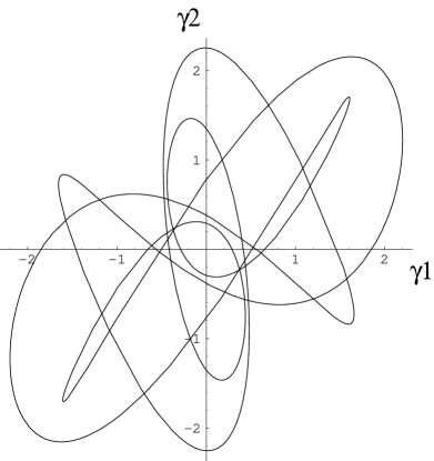
FIG. 13.: Parametrized curve $\gamma_{1}(t)=1.2\cos(5t+1)-\cos(3t)$, $\gamma_{2}(t)=1.3\cos(7t+0.3)-\cos(3t)$ as an example of the solution Eq.( C5) for a general degeneracy curve.

REFERENCES

- [1] D. P. Arovas, P. N. Bhatt, F. D. M. Haldane, P. B. Littlewood, and R. Rammal. Localization, wave function topology, and the integer quantized hall effect. Phys. Rev. Lett., 60, 1988.
- [2] J. E. Avron, R. Seiler, and B. Simon. Homotopy and quantization in condensed matter physics. Phys. Rev. Lett., 51, 1983.
- [3] B. Helffer and P. Kerdelhue and J. Sjoestrand. Le papillon de Hofstadter, revisite. (Hofstadter’s butterfly, revised). Mem. Soc. Math. Fr., Nouv. Ser., 43, 1990.
- [4] M. Berry. Quantal phase factors accompanying adiabatic changes. Proc. Roy. Soc. Lond., 45, 1984.
- [5] Bouzouina, A. and De Bievre, S. Equipartition of the eigenfunctions of quantized ergodic maps on the torus. Commun. Math. Phys. , 178(1):83–105, 1996.
- [6] Y. Colin de Verdière and B. Parisse. Équilibre instable en régime semi-classique - I. Concentration microlocale. Communications in Partial Differential Equations, 19(9-10):1535–1563, 1994.
- [7] Y. Colin de Verdière and B. Parisse. Équilibre instable en régime semi-classique - II. Conditions de Bohr-Sommerfeld. Annales de l’Institut Henri Poincaré- Physique Théorique, 61(3):347–367, 1994.
- [8] Y. C. de Verdière. Fibrés en droites et valeurs propes multiples. Séminaire de théorie spectrale -Institut Fourier Grenoble, pages 9–18, 92-1993.
- [9] D.J. Thouless. Topological interpretations of quantum Hall conductance. J. Math. Phys., 35 (10):5362–5372, 1994.
- [10] F. Faure. Generic description of the degeneracies in Harper-like models. J. Phys. A, Math. Gen., 27 (22):7519–7532, 1994.
- [11] F. Faure. Mécanique quantique sur le tore et dégénérescences dans le spectre. Séminaire de théorie spectrale et géométrie-Institut Fourier Grenoble, pages 19–63, 1992-93.
- [12] V. Gudmundsson and R. Gerhardts. Phys. Rev. B, 54:5223, 1996.
- [13] B. Helffer and J. Sjöstrand. Multiple wells in the semi-classical limit-I. Communication in Partial Differential Equation, 9(4):337–408, 1984.
- [14] D. Hofstadter. Energy levels and wave functions of bloch electrons in rational and irrational magnetic fields. Phys. Rev. B, 14-6, 1976.
- [15] J. Bellissard and A. van Elst and H. Schulz-Baldes. The noncommutative geometry of the quantum Hall effect. J. Math. Phys., 35 (10):5373–5451, 1994.
- [16] M. S. J. Kurchan, P. Leboeuf. Semiclassical approximation in the coherent state representation. Phys. Rev. A, 40, 1989.
- [17] M. Khomoto. Topological invariant and the quantization of the hall conductance. Ann. Phys. B, 160, 1985.
- [18] P. Lebœuf, J. Kurchan, M. Feingold, and D. P. Arovas. Phase-space localization: topological aspects of quantum chaos. Phys. Rev. Lett., 65, 1990.
- [19] P. Lebœuf and A. Voros. ”chaos-revealing multiplicative representation of quantum eigenstates”. J. Phys. A, 23, 1990.
- [20] M. Saraceno. Classical structures in the quantized Baker transformation. Ann. Phys. , 199 (1):37–60, 1990.
- [21] A. Martinez. Estimates on complex interactions in phase space. Math. Nachr., 167:203–254, 1994.
- [22] T. Paul and A. Uribe. A construction of quasi-modes using coherent states. Ann. Inst. H. Poincaré, Phys. théor, 59 (4):357–381, 1993.
- [23] S. Nakamura. On an example of phase-space tunneling. Ann. Inst. Henri Poincare, Phys. Theor. , 63(2):211–229, 1995.
- [24] T. Schlosser, K. Ensslin, J. Kotthaus, and M. Holland. Europhys. Lett., 33:683, 1996.
- [25] B. Simon. Holonomy, the quantum adiabatic theorem and berry’s phase. Phys. Rev. Lett., 51, 1983.
- [26] D. Springsguth, R. Ketzmerick, and T. Geisel. Hall conductance of bloch electrons in a magnetic field. Phys. Rev. B, 56:2036, 1997.
- [27] D. J. Thouless, M. Khomoto, M. P. Nightingale, and M. den Nijs. Quantized hall conductance in a two-dimensional periodic potential. Phys. Rev. Lett., 49, 1982.
- [28] V. Bargmann. On a Hilbert space of analytic functions and an associated integral transform. Commun. Pure Appl. Math., 14:197–214, 1961.
- [29] J. von Neumann and E. Wigner. Phys. Z., 30, 1929.
- [30] A. Voros. Wentzel-kramers-brillouin method in the bargmann representation. Phys. Rev. A, 40, 1989.
- [31] M. Wilkinson. Critical properties of electron eigenstates in incommensurate systems. Proc. R. Soc. Lond. A, 391, 1984.
- [32] M. Wilkinson and E. Austin. Phase space lattices with threefold symmetry. J. Phys. A, 23, 1990.