[

Dynamical Correlations in a Half-Filled Landau Level

Abstract

We formulate a self-consistent field theory for the Chern-Simons fermions to study the dynamical response function of the quantum Hall system at $\nu=\frac{1}{2}$. Our scheme includes the effect of correlations beyond the random-phase approximation (RPA) employed to this date for this system. We report results on the density response function, dynamic structure factor, the static structure factor, the longitudinal conductivity and the interaction energy of the system. The longitudinal conductivity calculated in this scheme shows linear dependence on the wave vector, like the experimentals results and the RPA, but the absolute values are higher than the experimental results.

]

Despite rapid progress in the field of quantum Hall effect in recent years, proper understanding of the state at half-filled Landau level still remains a challanging problem. A modified Fermi-liquid theory of Chern-Simons (CS) fermions, put forward by Halperin, Lee and Read (HLR) [2] explained some of the anomalies observed in surface acoustic wave experiments (SAW) around the filling factor $\nu=\frac{1}{2}$ [3]. One very interesting result of this theory was that at $\nu=\frac{1}{2}$ the average effective magnetic field acting on the fermions vanishes and one expects a Fermi surface for those fermions. This result within the mean-field approach was later verified in experiments [3], where one finds indications, albeit indirect, for the existence of a Fermi surface. In going beyond the mean field theory one has to include interactions via the Chern-Simons field in order to describe the dynamic response functions, transport properties, etc. HLR studied the response functions within the random phase approximation (RPA) which takes care of the direct Coulomb interaction and the fluctuations in Chern-Simons field. In the work of HLR the response functions were analyzed only in the long-wavelength limit. The RPA scheme was found to explain the wave vector dependence of the longitudinal conductivity derived from the SAW experiments [2]. The absolute value of the calculated conductivity was, however, lower than the experimental results by a factor of two. The apparent success of HLR approach has marked the beginning of intense activities in the field, so much so that often the embellishments tend to overtake the actual facts.

In this letter, we report our studies of the density response function, the dynamic structure factor, the static structure factor, and the longitudinal conductivity for the quantum Hall system at the filling factor $\nu=\frac{1}{2}$, where we include correlations beyond the RPA scheme for the Chern-Simons fermions. In doing that, we have developed for the first time a variation on the theme of the celebrated self-consistent field theory of Singwi, Tosi, Land and Sjölander (STLS) [4] in the quantum Hall regime and at a half-filled Landau level. The efficacy of STLS approach over the RPA scheme in describing correctly the dynamical properties is well established [5]. Our results for longitudinal conductivity show linear wave vector dependence, as in experiments and also in the RPA scheme, but the absolute values are higher than the experimental results. Most of the RPA results for the static and dynamical functions are also reported here for the first time.

We begin by presenting a few essential steps of the HLR approach to establish our notation. The CS transformation for spinless fermions is defined by (henceforth we use units where $\hbar=e=1$) [2]

$$\tilde{\Psi}^{\dagger}({\bf r})=\Psi^{\dagger}_{e}({\bf r})\exp\left[-2{\rm i}\int d{\bf r}^{\prime}\arg({\bf r}-{\bf r}^{\prime})\rho({\bf r}^{\prime})\right]$$ (1)

where $\Psi^{\dagger}_{e}({\bf r})$ is the electron creation operator, $\tilde{\Psi}^{\dagger}({\bf r})$ is the transformed fermion operator, and $\arg({\bf r})$ is the angle that vector ${\bf r}$ forms with the $x$-axis. The kinetic part of the Hamiltonian, which alters due to the transformation, is then

$${\cal H}_{\rm kin}=\frac{1}{2m_{b}}\int d{\bf r}\,\tilde{\Psi}^{\dagger}({\bf r})\left[-{\rm i}\nabla+\delta{\bf A}({\bf r})\right]^{2}\tilde{\Psi}({\bf r})$$ (2)

where $m_{b}$ is the electron band mass and

$$\delta A_{i}({\bf r})=\int d{\bf r}^{\prime}\phi_{i}({\bf r}-{\bf r^{\prime}})\rho({\bf r}^{\prime})$$ (3)

[$\phi_{i}({\bf r})=2\nabla_{i}\arg({\bf r})$] is the CS field. Expanding the right hand side of Eq. (2) and keeping only up to second-order contribution, one gets

$${\cal H}= - \frac{1}{2m_{b}}\int d{\bf r}\,\tilde{\Psi}^{\dagger}({\bf r})\nabla^{2}\tilde{\Psi}({\bf r})$$ (4)

$$+ \sum_{{\bf k}\neq 0}{\rm i}v_{1}(k)j^{T}_{\bf k}\rho_{-\bf k}+{1\over 2}[v_{0}(k)+v_{2}(k)]\rho_{\bf k}\rho_{-\bf k}$$ (5)

where $j^{T}_{\bf k}=\hat{\bf k}\times{\bf j}_{\bf k}$ is the transverse component of the transformed current operator

$${\bf j}({\bf r})=\tilde{\Psi}^{\dagger}({\bf r})\frac{{\rm i}\nabla}{m_{b}}\tilde{\Psi}({\bf r}),$$ (6)

(note that HLR used the diamagnetic current ${\bf J}+\rho_{0}{\bf A}/m_{b}$, with $\rho_{0}$ being the equilibrium density), where $v_{0}=2\pi/k$ is the Coulomb potential, $v_{1}(k)=4\pi/k$, and $v_{2}(k)=(4\pi)^{2}\rho_{0}/m_{b}k^{2}$ [i$\epsilon_{jh}\hat{k}_{h}v_{1}(k)$ is the Fourier transform of $\phi_{j}({\bf r})$]. This Hamiltonian describes a system with the same density as the original system where there is no magnetic field but contains a potential $v_{1}(k)$ which couples the density fluctuations to the transverse currents. This observation is the key ingredient for the exploitation of schemes that are normally applied to the electron gas in a zero magnetic field.

We intend to compute the response function matrix $\chi$, which gives the density and transverse current responses $\rho({\bf k},\omega)$ and $j_{T}({\bf k},\omega)$ to external perturbation scalar and transverse vector potentials $V^{\mathrm{pert}}$ and $A_{T}^{\mathrm{pert}}$ via

$$\left(\rho({\bf k},\omega)\atop j_{T}({\bf k},\omega)\right)=\chi({\bf k},\omega)\cdot\left(V^{\mathrm{pert}}({\bf k},\omega)\atop A_{T}^{\mathrm{pert}}({\bf k},\omega)\right)$$ (7)

where the longitudinal current and vector potential have been eliminated using the continuity equation and gauge invariance. Following the original derivation of STLS, we start from the equation of motion for the one-body Wigner distribution function

$$f^{(1)}({\bf r},{\bf p};t)=\sum_{\bf k}e^{{\rm i}{\bf k}{\bf r}}\langle{a^{\dagger}_{{\bf p}-{\bf k}/2}(t)a_{{\bf p}+{\bf k}/2}(t)}\rangle,$$ (8)

which determines the density $\rho({\bf r},t)=\sum_{\bf p}f^{(1)}({\bf r},{\bf p};t)$ and the current ${\bf j}({\bf r},t)=\sum_{\bf p}{\bf p}f^{(1)}({\bf r},{\bf p};t)/m_{b}$. In the semiclassical limit the Heisenberg equation of motion for the electron operators $a_{\bf k}$ and $a^{\dagger}_{\bf k}$ gives

$${\partial\over\partial t}f^{(1)}({\bf r},{\bf p};t)={{\bf p}\cdot\nabla_{\bf r}\over m_{b}}f^{(1)}({\bf r},{\bf p};t)$$ (9)

$$+\!\int\!d{\bf r^{\prime}}\!\sum_{\bf p^{\prime}}\left[{({\bf p}\!-\!{\bf p}^{\prime})_{j}\over m_{b}}(\nabla_{i}\phi_{j})({\bf r}\!-\!{\bf r^{\prime}})\nabla_{{\bf p},i}{\vbox to14.39996pt{}}\right.$$ (10)

$$\left.+[\nabla_{i}(v_{0}+v_{2})]({\bf r}-{\bf r^{\prime}})\nabla_{{\bf p},i}{\vbox to14.39996pt{}}\right]f^{(2)}({\bf r},{\bf p};{\bf r^{\prime}},{\bf p^{\prime}};t)$$ (11)

$$+\nabla_{{\bf p},i}f^{(1)}\nabla_{i}V^{\mathrm{pert}}({\bf r},t)+{{\bf p}_{j}\over m_{b}}\nabla_{{\bf p},i}f^{(1)}\nabla_{i}A_{j}^{\mathrm{pert}}({\bf r},t)$$ (12)

where $\nabla_{{\bf p},i}=\partial/\partial{\bf p}_{i}$, and

$$f^{(2)}({\bf r},{\bf p};{\bf r^{\prime}},{\bf p^{\prime}};t)=\sum_{{\bf k},{\bf k^{\prime}}}e^{{\rm i}{\bf k}{\bf r}}e^{{\rm i}{\bf k^{\prime}}{\bf r^{\prime}}}\hskip 62.59596pt$$ (13)

$$\hskip 22.76228pt\times\langle{a^{\dagger}_{{\bf p}-{\bf k}/2}(t)a_{{\bf p}+{\bf k}/2}(t)a^{\dagger}_{{\bf p^{\prime}}-{\bf k^{\prime}}/2}(t)a_{{\bf p^{\prime}}+{\bf k^{\prime}}/2}(t)}\rangle$$ (14)

is the two-body distribution function. The key step in the STLS approximation consists in the decoupling

$$f^{(2)}({\bf r},{\bf p};{\bf r^{\prime}},{\bf p^{\prime}};t)\simeq f^{(1)}({\bf r},{\bf p};t)f^{(1)}({\bf r^{\prime}},{\bf p^{\prime}};t)g({\bf r}-{\bf r^{\prime}})$$ (15)

i.e., in the assumption that the correlations in the perturbed, time-dependent state are identical to those in the unperturbed, equilibrium state, and are therefore described by the static pair correlation function $g(r)$. Notice that setting $g(r)=1$ in Eq. (15) one recovers the RPA where short-range correlations are neglected.

Equation (12) is equivalent to the response of noninteracting electrons to the effective potentials

$$\nabla_{i}V^{\mathrm{eff}} = \nabla_{i}V^{\mathrm{pert}}+\int d{\bf r^{\prime}}\rho({\bf r^{\prime}})g({\bf r}\!-\!{\bf r^{\prime}})\nabla_{i}(v_{0}+v_{2})({\bf r}\!-\!{\bf r^{\prime}})$$ (17)

$$+\sum_{j=1}^{2}{\bf j}^{T}_{j}({\bf r^{\prime}})g({\bf r}-{\bf r^{\prime}})\nabla_{i}\phi_{j}({\bf r}\!-\!{\bf r^{\prime}})$$

and

$$\nabla_{i}A_{j}^{\mathrm{eff}}=\nabla_{i}A_{j}^{\mathrm{pert}}+{\cal P}_{T}\int d{\bf r^{\prime}}\rho({\bf r^{\prime}})g({\bf r}-{\bf r^{\prime}})\nabla_{i}\phi_{j}({\bf r}\!-\!{\bf r^{\prime}})$$ (18)

where the continuity equation has been used to eliminate the longitudinal part of the current, and ${\cal P}_{T}$ indicates projection onto the subspace of transverse vector potentials. In matrix notation this implies $\chi=\chi^{0}[1+U\chi]$, or equivalently

$$\chi=\chi^{0}\left[1-U\chi^{0}\right]^{-1},$$ (19)

where

$$\chi^{0}=\left(\begin{array}[]{cc}\chi^{0}_{\rho\rho}&0\\ 0&\chi^{0}_{T}\end{array}\right)$$ (20)

is the ideal-gas response function which is known analytically [6]. The matrix of the effective potentials, from Eqs. (17–18) is

$$U=\left(\begin{array}[]{cc}w_{0}(k)+w_{2}(k)&{\rm i}w_{1}(k)\\ -{\rm i}w_{1}(k)&0\end{array}\right),$$ (21)

where $w_{\alpha}(k)=[1-G_{\alpha}(k)]v_{\alpha}(k)$ and the local field factors $G_{\alpha}(k)$ are given by

$$G_{\alpha}(k)=\sum_{\bf p}[1-S({\bf p})]{[{\bf k}\cdot({\bf k}-{\bf p})]^{(a_{\alpha}+b_{\alpha})/2}\over k^{a_{\alpha}}\left|{\bf k}-{\bf p}\right|^{b_{\alpha}}}$$ (22)

with $a_{0}=b_{0}=1$, $a_{1}=b_{1}=2$, $a_{2}=0$, and $b_{2}=2$, and $S(k)$ is the static structure factor, i.e., the Fourier transform of the pair correlation function $g(r)$. Using the rotational invariance of $S(k)$ it is easy to show that in the $k\to 0$ limit $G_{0}$ is linear in $k$, $G_{2}$ is quadratic in $k$, and $G_{1}$ has a finite limit, $G_{1}(0)=[1-g(0)]/2=1/2$. Notice that the RPA approximation of HLR amounts to $G_{\alpha}(k)=0$, i.e., $w_{\alpha}(k)=v_{\alpha}(k)$.

The static structure factor entering Eq. (22) is obtained from the fluctuation-dissipation theorem,

$$S(k)=-{1\over\rho_{0}\pi}\int_{0}^{\infty}{\bf Im\,}\chi_{\rho\rho}(k,\omega)d\omega$$ (23)

where $\chi_{\rho\rho}(k,\omega)$ is the density-density response function given by Eq. (19),

$$\chi_{\rho\rho}(k,\omega)={\chi_{\rho\rho}^{0}(k,\omega)\over 1-\chi^{0}_{\rho\rho}\left[w_{0}(k)+w_{2}(k)+w_{1}(k)^{2}\chi^{0}_{T}\right]}.$$ (24)

Equations (19-24) are then solved self-consistently for a given value of the dimensionless coupling strength, $r_{s}=r_{0}/a_{B}=2{e^{2}/\ell_{0}\omega_{c}}$, where $a_{B}=1/m_{b}e^{2}$ is the Bohr radius, $r_{0}=(\pi\rho_{0})^{-1/2}$ is the average interparticle spacing, $\ell_{0}=|B|^{-\frac{1}{2}}$ is the magnetic length and $\omega_{c}=B/m_{b}$ is the cyclotron frequency. The relevant values of $r_{s}$ can be estimated in two ways: following HLR [2] we can write, $r_{s}=2/C$, where $C\simeq 0.3$ is related to the effective mass. Alternatively, we can obtain $r_{s}$ from a realistic estimate of $\omega_{c}$ and $e^{2}/\ell_{0}$, which is typically, $r_{s}=1\div 3$. The numerical results show little variation between the two cases but for definiteness we consider the first choice.

Since the density is not affected by the CS transformation of Eq. (1), the density-density response function of the transformed system is identical to that of the original electron system, and therefore contains information about physical properties such as the structure factor, the conductivity, etc. In the following we present and discuss our results for various quantities derived from $\chi_{\rho\rho}$, and can therefore drop the distinction between the two systems from now on.

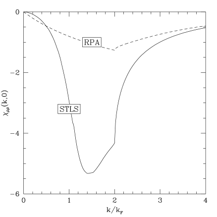
FIG. 1.: Static density-density response function $\chi_{\rho\rho}(k,0)$ as a function of $k/k_{F}=k\ell_{0}$, calculated in the RPA (dashed curve) and in STLS (full curve) for $r_{s}=7$. The discontinuity in the derivative at $k=2k_{F}$ corresponds to the Fermi surface.

In the static long-wavelength limit ($\omega\ll kv_{F}$, $k\ll k_{F}$, $k_{F}=m_{b}v_{F}=1/\ell_{0}$ being the Fermi momentum) one has

$$\chi^{0}_{\rho\rho}(k,\omega)\simeq-{m_{b}\over 2\pi}\left(1+{\rm i}{\omega\over kv_{F}}\right)$$ (25)

and

$$\chi^{0}_{T}(k,\omega)\simeq-{\rho_{0}\over m_{b}}\left(1+{\rm i}{2\omega\over kv_{F}}\right).$$ (26)

In the RPA, $v_{2}=\rho_{0}v_{1}^{2}/m_{b}$, hence the leading term in the denominator of Eq. (24) cancels, and $\chi_{\rho\rho}(k,0)$ vanishes linearly for small $k$. If local field factors are included, this cancellation does no longer take place and one gets $\chi_{\rho\rho}(k,0)\simeq-(m_{b}/3\pi)k^{2}/k_{F}^{2}$. The results are presented in Figure 1, where one clearly sees the difference in the limit $k\to 0$. We note that the $k^{2}$ dependence of the compressibility at $\nu=1/2$ has been observed also by other authors[7] in the dipole nature of $\nu=1/2$ state, which arises primarily due to projection to the lowest Landau level. Further, we find that excluding the cyclotron contribution, $\int{\bf Im\,}\chi_{\rho\rho}\omega d\omega\propto q^{4}$ and $\int{\bf Im\,}\chi_{\rho\rho}d\omega\propto q^{3}$ apart from possible logarithmic terms.

The longitudinal conductivity, which is relevant to surface-acoustic-wave experiments is given by $\sigma_{xx}^{-1}={\rm i}(k^{2}/\omega)[\chi_{\rho\rho}^{-1}(k,\omega)-\chi_{\rho\rho}^{-1}(k,0)]$. Since the speed of sound $c_{s}$ is small compared to the Fermi velocity $v_{F}$ and $k\ll k_{F}$, we can use the limiting forms (25-26) into Eq. (24). This leads to the result $\sigma_{xx}(k,c_{s}k)\simeq k/2\pi k_{F}$, which has the same linear dependence on $k$, but is twice the experimental values[3]. The RPA result of HLR is $\sigma^{RPA}_{xx}(k,c_{s}k)\simeq k/8\pi k_{F}$. A quantitative agreement with experiment can however be achieved if the CS interaction $\phi_{j}({\bf r})$ is softened at small separation.

Using the well-known asymptotic behaviors, $\chi^{0}_{\rho\rho}=\rho_{0}k^{2}/m_{b}\omega^{2}$ and $\chi^{0}_{T}=O(k^{2})$, valid for $k\ell_{0}\ll 1$, $kv_{F}\ll\omega$, one sees that the dynamical structure factor

$$S(k,\omega)=-\frac{1}{\rho_{0}\pi}{\rm\bf Im}\,\chi_{\rho\rho}(k,\omega)$$ (27)

has a pole at the cyclotron frequency $\omega=\omega_{c}$, describing inter-Landau-level excitations, which – at $k=0$ – is unaffected by correlations, and is in agreement with Kohn’s theorem. The mode dispersion, which is computed by locating the zeroes of the denominator in Eq. (24), turns out to be significantly lower than the RPA result (see inset of Fig. 2). Our finite-$k$ results are presented in Figure 2 where we have a $\delta$-function peak at $\omega\sim\omega_{c}$, corresponding to the cyclotron motion and a continuum of particle-hole excitations in the range

$$\frac{k^{2}}{2m_{b}}-v_{F}k\leq|\omega|\leq\frac{k^{2}}{2m_{b}}+v_{F}k\,.$$ (28)

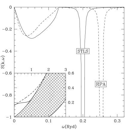
FIG. 2.: Dynamic structure factor $S(k,\omega)$ for $k=0.6k_{F}$, as a function of $\omega$ (in Rydberg) in RPA (dashed curve) and STLS (full curve). The $\delta$-function peak corresponding to the inter-Landau-level mode has been artificially broadened for clarity and contains most of the spectral strength. The inset shows the excitation spectrum, composed of the particle-hole continuum plus the sharp cyclotron mode.

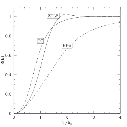
FIG. 3.: Static structure factor $S(k)$ as a function of $k/k_{F}=k\ell_{0}$ in the RPA and the STLS scheme. The results are also compared with the results from Ref. [8] (TC).

Our results for the static structure factor $S(k)$ are plotted in Fig. 3. Here we compare our RPA results, calculated from Eqs. (23-24) with $w_{\alpha}=v_{\alpha}$, and the STLS results, at $r_{s}=7$. These results are also compared with $S(k)$ calculated for a modified Laughlin state at $\nu=\frac{1}{2}$ [8], proposed by Read [9]. All these curves obey the leading $(k\ell_{0})^{2}/2$ behavior at small $k$. As expected, the STLS scheme includes substantial amount of correlations and hence is significantly higher than the RPA results near $k=2k_{F}$.

Knowledge of the structure factor $S(k)$ allows us to compute the potential energy per particle, $\langle PE\rangle={1\over 2}\sum_{k}v_{0}(k)[S(k)-1]$. The full interaction energy (defined as the total energy minus the noninteracting term $\hbar\omega_{c}/2$) is then obtained via coupling constant integration,

$$E_{\rm int}(r_{s})={1\over r_{s}}\int_{0}^{r_{s}}dr_{s}^{\prime}\langle PE(r_{s}^{\prime})\rangle$$ (29)

(we measure energies in units of $e^{2}/\ell_{0}$). The STLS result $E_{\rm int}\simeq-0.48$ compares favorably with finite-size exact diagonalization studies[10], $E_{\rm int}=-0.466$. The RPA overestimates appreciably the interaction energy, and gives $E_{\rm int}\simeq-0.76$. At the same $r_{s}$, the STLS potential energy is $\langle PE\rangle=-0.49$, showing that the inter-Landau-level kinetic energy is a minor contribution.

In summary, we have presented a self-consistent scheme for the calculation of the dynamical response function of a quantum Hall fluid at $\nu={1\over 2}$, based on a generalization of the STLS method to the case of Chern-Simons fermions. Our results exhibit significant differences with the RPA computations, in particular on the longitudinal conductivity, the static response function and the structure factor.

We wish to thank Peter Fulde for his kind hospitality at the Max-Planck-Institute for Physics of Complex Systems in Dresden.

REFERENCES

[1]
On leave from: Institute of Mathematical Sciences, Taramani, Madras
600 113, India
[2] B. I. Halperin, P. A. Lee, and N. Read, Phys. Rev. B 47,
7312 (1993).
[3]
R. L. Willett, Adv. Phys. 46, 447 (1997).
[4]
K. S. Singwi, M. P. Tosi, R. H. Land, and A. Sjölander, Phys. Rev. 179, 589 (1968); K. S. Singwi and M. P. Tosi, Solid State Phys. 36,
177 (1981).
[5]
A. vom Felde, J. Sprösser-Prou, and J. Fink, Phys. Rev. B 40, 10181
(1989).
[6]
F. Stern, Phys. Rev. Lett. 18, 546 (1967);
R. Nifosì, S. Conti, and M. P. Tosi, cond-mat/9807085.
[7]
V. Pasquier and F. D. M. Haldane, cond-mat/9712169; R. Shankar and G. Murthy,
Phys. Rev. Lett. 79, 4437 (1997); cond-mat/9802244; see also,
B. I. Halperin and A. Stern, Phys. Rev. Lett. 80, 5457 (1998).
[8]
T. Chakraborty, Phys. Rev. B 57, 8812 (1998).
[9]
N. Read, Semicond. Sci. Technol. 9, 1859 (1994).
[10]
R. Morf and N. d’Ambrumenil, Phys. Rev. Lett. 74, 5116 (1995).