Pairing Correlations and the Pseudo-Gap State: Application of the “Pairing Approximation” Theory

Abstract

We investigate the pseudogap onset temperature $T^{*}$, the superconducting transition temperature $T_{c}$ and the general nature of the pseudogap phase using a diagrammatic BCS-Bose Einstein crossover theory. This decoupling scheme is based on the “pairing approximation” of Kadanoff and Martin, further extended by Patton (KMP). Our consideration of the KMP “pairing approximation” is driven by the objective to obtain BCS like behavior at weak coupling, (which does not necessarily follow for other diagrammatic schemes). Two coupled equations, corresponding to those for the single particle and pair propagators, must be solved numerically, along with the number equation constraint. The variation of small to large coupling constant $g$ is explored, whereby the system is found to cross over from BCS to Bose-Einstein behavior. Our numerical calculations proceed in two stages: first we investigate the “lowest order theory”, which is appropriate at temperatures well above $T_{c}$. We use this theory to determine where the Fermi liquid state first breaks down. This breakdown, which occurs at $T^{*}$ and is associated with intermediate values of the coupling, corresponds to a splitting of the single peaked (Fermi liquid) electronic spectral function into two peaks well separated by a gap, as might be expected for the pseudogap phase. Indeed, our calculations provide physical insight into the pseudogap state which is characterized by the presence of metastable pairs or “resonances”, which occupy states around the Fermi energy; in this way they effectively reduce the single particle density of states. The superconducting instability $T_{c}$ is evaluated in the second stage of our calculations. Here we introduce “mode coupling” effects, in which the long lived pairs are affected by the single particle pseudogap states and vice versa. Our $T_{c}$ equations, which turn out to be rather simple as a result of the KMP scheme, reveal a rich structure as a function of $g$ in which the pseudogap is found to compete with superconductivity. Our results are compared with alternate theories in the literature.

cond-mat/9805018 ]

I Introduction

Pseudogap phenomena were reported in the first generation of underdoped high $T_{c}$ samples[1], although they received little attention at that time. These early experiments[1] on underdoped cuprates demonstrated a suppression in the magnetic susceptibility with decreasing temperature ($T<T^{*}$) which was suggestive of some form of singlet pairing in the normal state. These first indications of the pseudogap state were strictly associated with magnetic probes. Hence the phrase “spin gap” was used to describe them and related frequency dependent magnetic phenomena[2]. More recently, it has become clear that similar effects[3] are present in the charge response as well. Today the spin gap is more broadly interpreted to correspond to some form of excitation gap (i.e., pseudogap) in both charge and spin channels. It can and has been debated as to whether the effects are equally profound in each.

Among the most revealing data on the pseudogap state are angle resolved photoemission experiments[4, 5] (ARPES) which demonstrate that below $T^{*}$ the pseudogap is present in the energy dispersion of the normal state electrons and that, moreover, it seems to have the same (d-wave) symmetry as the superconducting state, and evolves more or less continuously through $T_{c}$ into a superconducting excitation gap. Finally, these data show that the pseudogap is attached to an underlying Luttinger volume Fermi surface, although there are many aspects about the high temperature regime ($T>T^{*}$), (where the pseudogap is essentially absent), which do not correspond to a canonical Fermi liquid.

Theories of the cuprate pseudogap can be broadly divided into two groups: those that associate this state with magnetic pairing of some sort[6, 7, 8, 9, 10, 11] and those which view the pseudogap as deriving from some form of precursor superconductivity [12, 13, 14, 15, 16, 17, 18, 19, 20, 21, 22, 24]. (In reality the division between these two classes is somewhat blurred, since in many scenarios magnetic pairing is a natural requisite for superconductivity). The present paper belongs to this second category. It is our contention that this second scenario deserves careful attention in large part because mean field descriptions of the transition (which neglect precursor or pairing correlation effects) are not expected to be applicable to short coherence length, quasi 2d superconductors such as the cuprates. Moreover, ARPES data suggest a smooth evolution of the pseudo- into the superconducting gap. Finally, these systems ultimately undergo a superconducting, not magnetic transition. At the very least it is clear that the pseudogap state will never be fully characterized unless precursor superconducting effects are properly calibrated.

Within the precursor superconductivity school, there are, moreover, two distinct classes. The first of these is based on the short coherence length $\xi$ which is naturally associated with modest size Cooper pairs and, therefore, a superconducting state intermediate between the BCS (large pair) and Bose-Einstein (small pair) descriptions. The second class is based on the anomalously low plasma frequency $\omega_{p}$ which suggests that phase fluctuations play an important role. In this way the amplitude of the order parameter is established at $T^{*}$, while phase coherence occurs at the much lower temperature $T_{c}$. In reality, both $\xi$ and $\omega_{p}$ are small and some initial work by our group[25] has treated these two parameters on a more even footing.

While, there have been no decisive arguments in favor of one or the other of the two precursor superconductivity schools, in this paper we explore the “BCS Bose-Einstein crossover” scenario, in large part because it lends itself to more detailed diagrammatic and therefore quantitative calculations and insights. There is a long history associated with this small pair theory. Leggett[26] first proposed a variational ground state wave function which exhibited a smooth interpolation between the BCS and Bose-Einstein regimes. An essential component of his approach was the introduction of a self consistent equation for the chemical potential to be solved in conjunction with the variational conditions [27]. This $\mu$ differs significantly from the Fermi energy in all but the very weak coupling limit. Nozieres and Schmitt-Rink (NSR) [28] extended Leggett’s ideas to non-zero temperature and thereby deduced a transition temperature $T_{c}$ which varied continuously with increasing coupling constant $g$ from the BCS exponential dependence on $g$ to the Bose-Einstein asymptote. Randeria and co- workers[13] were among the first to apply the NSR approach, derived via a saddle point scheme, to the cuprates, which were associated with intermediate values of $g$. Subsequent extensive numerical[29] and analytical[30] studies have addressed the intermediate $g$ regime beyond the NSR approximations and find a variety of aspects of pseudogap behavior.

An important goal of the present paper is to address the cross-over problem within a specific diagrammatic scheme, which is amenable to quasi-analytic calculations and physical interpretation. In the process we are able to compute the electronic self energy, spectral function and a quantitative phase diagram for $T_{c}$ and $T^{*}$ as a function of $g$. We refer to this decoupling scheme as the “pairing approximation” theory. It is based on early work by Kadanoff and Martin[31] and has been argued by these authors to be the most appropriate treatment for introducing pairing correlations of the kind encountered in a conventional superconducting state. Moreover, this approximation has been extensively applied by Patton[32, 33] to the problem of $T>T_{c}$ fluctuations in low dimensional, dirty superconductors. As will be discussed in detail in a future paper[34] which addresses the superconducting state, the present diagram scheme leads naturally to Leggett’s[26] description of the interpolated ground state. This is in contrast to alternative diagrammatic approaches [35, 36, 37, 38, 39] which, below $T_{c}$, do not recover the BCS limit in the weak coupling regime.

As a result of these calculations, a simple physical picture of the pseudogap phase emerges. This is a regime of intermediate coupling $g$ which is characterized by a normal state that is somewhere between the “free” fermions of the BCS limit and the “pre-formed” pairs of the Bose-Einstein case. A natural description of the interpolated state is to presume that it corresponds to “resonantly” scattered or meta-stable pairs. Indeed, our calculations of the electronic self energy and spectral function[22] show that the presence of resonant scattering (as deduced from the character of the pair propagator or T-matrix), correlates rather well with the break-down of the Fermi liquid phase. Once the pairs are meta- stable they block available states around the Fermi surface which would otherwise be occupied by single electrons and thereby introduce a pseudogap into the electronic spectrum.

While this interpretation of the density of states depression is in the same spirit as earlier work[32] on superconducting fluctuation induced spectral gaps, the present description differs in an important way. Long lived pair states in ordinary superconductors occur in the vicinity of $T_{c}$ as a consequence of critical slowing down. By contrast, here they are found to occur at much higher temperatures simply because the coupling $g$ is sufficiently strong to bind the pairs into a meta-stable state. This picture must necessarily be distinguished from the phase fluctuation picture of Emery and Kivelson[12] as well as from the “pre-formed” pair models of other groups[15, 16, 17, 18, 19]. Our pairs correspond to microscopic as distinct from mesoscopically established regions of superconductivity. Moreover, the resonant pairs of the present model have a finite lifetime and spatial extent and do not obey Bose statistics.

II Theoretical Framework

We consider a generic Hamiltonian consisting of fermions in a three dimensional, jellium gas in the presence of an s-wave attractive interaction, $V_{\bf k,k^{\prime}}=g\varphi_{\bf k}\varphi_{\bf k^{\prime}}$, where $\varphi_{\bf k}=(1+k^{2}/k^{2}_{0})^{-1/2}$ and $g<0$ is the coupling strength expressed in units of $g_{c}=-4\pi/mk_{0}$. Effects associated with quasi two dimensional lattices and d-wave pairing have also been addressed within this formalism and will be discussed in a companion paper[40]. The results which we present here are generally robust, although the relevant energy scales decrease considerably as the system becomes more two dimensional. Because we consider only this simplest case, we defer the discussion of direct comparison with ARPES data to future work.

Following earlier work[31, 32] by Kadanoff and Martin and by Patton, the system can be characterized by the integral equations of the “pairing approximation” which describe a coupling between the electronic self energy $\Sigma$ and T matrix $t$. We add to these equations the usual expression for particle number conservation

$$\Sigma_{{\bf k},i\omega_{l}} \;=\; T\sum_{{\bf q},\Omega_{m}}t_{{\bf q},i\Omega_{m}}G^{(0)}_{{\bf q-k},i\Omega_{m}-i\omega_{l}}\varphi^{2}_{{\bf k-q}/2}\;,$$ (2)

$$t^{-1}_{{\bf q},i\Omega_{m}} = g^{-1}+T\sum_{{\bf k},\omega_{l}}G_{{\bf k},i\omega_{l}}G^{(0)}_{{\bf q-k},i\Omega_{m}-i\omega_{l}}\varphi^{2}_{{\bf k-q}/2}\;,$$ (3)

$$n = \frac{1}{\beta}\sum_{{\bf k},\omega_{l},\sigma}G_{{\bf k},i\omega_{l}}\;.$$ (4)

where the Green’s function is given by $G^{-1}_{{\bf k},i\omega_{l}}=G^{(0)-1}_{{\bf k},i\omega_{l}}-\Sigma_{{\bf k},i\omega_{l}}$, the bare propagator is $G^{(0)-1}_{{\bf k},i\omega_{l}}=i\omega_{l}-\epsilon_{\bf k}$, and $\Omega_{m}/\omega_{l}$ are the even/odd Matsubara frequencies, with electronic dispersion given by $\epsilon_{\bf k}=k^{2}/2m-\mu$.

These first two equations may be readily written diagrammatically as shown in Figure  1. For completeness we also indicate the diagrams of the “lowest order theory”, Figure  1(b), which will be used initially to build intuition.

Although, these integral equations must in general be solved numerically, it will be possible to arrive at considerable analytic insight. The goal of this paper is to solve these three coupled equations as a function of arbitrary coupling $g$ for two different temperature regimes. Our calculations will accordingly proceed in two stages. First we discuss the “lowest order” conserving theory (Section  III) where all Green’s functions in Eqs.(II) are replaced by bare propagators[22]. This theory is adequate for describing the break down of the Fermi liquid at $T^{*}$ and for higher temperatures. In the next stage we (Section  IV) introduce feedback or “mode coupling” effects in which the pair propagator is allowed to depend on the single particle self energy and vice versa. This feedback is necessarily important within the pseudogap phase and all the way down to $T_{c}$. For a range of temperatures at and above $T_{c}$ but less than $T^{*}$, where the pseudogap is still well established, feedback or mode coupling effects can be readily introduced via a simple parameterization of the self energy. We will see below that this simplicity occurs in large part because of the presence of one “bare” Green’s function in the first two equations above. This parameterization will be justified numerically in considerable detail. By contrast, a direct numerical attack on the problem using the three full equations is difficult to implement as well as assess because of restrictions to a finite number of Matsubara frequencies[23]. Moreover, it does not provide the same degree of physical insight, nor can it be done in as controlled a fashion.

The present scheme should be contrasted with two alternative approaches in the literature. The approach of Nozieres and Schmitt- Rink[28] is embedded[36] in the limit of Eqs. (II) which corresponds to the lowest order theory and in which also the right hand side of the number equation is approximated by the first two terms in a Dyson expansion

$$G=G^{(0)}+G^{(0)}\Sigma^{(0)}G^{(0)}$$ (5)

As a consequence of this last approximation there are general problems with the violation of conservation laws which can be immediately corrected by summing the full Dyson equation for $G$. In this way our conserving “lowest” order theory is obtained as a first stage improvement over the NSR scheme. Along related lines, the Baym-Kadanoff criteria have been applied[41, 32] to verify conservation laws in the context of the full, mode coupled theory in Eqs. (II). Finally, Ward identities can be imposed in conjunction with these full equations to arrive at a satisfactory description of two particle properties as has been extensively investigated in Ref. [32].

Much attention has been paid to an alternative scheme in which all bare Greens functions in Eqs. (II) are replaced by their dressed counterparts. This approach, often referred to as the fluctuation exchange scheme or FLEX, has been studied by direct numerical methods in finite size systems[39] as well as for the purposes of computing $T_{c}$[35]. While it is a “$\Phi$ derivable” theory in the sense of Baym[42] it was noted some time ago[31] to be inconsistent with BCS theory, even in the weak coupling limit. It is, consequently, useful to explore the present Kadanoff-Baym-Patton approach both as a point of comparison for results obtained within the FLEX scheme, and because it appears to be more analytically tractable and more readily interpreted within the context of conventional theories of superconductivity.

III The Lowest Conserving Order

The single particle self-energy, $\Sigma_{{\bf k},\omega}$, at the lowest conserving level of approximation corresponds to

$$\Sigma^{(0)}_{{\bf k},i\omega_{l}}=T\sum_{{\bf q},\Omega_{m}}t^{(0)}_{{\bf q},i\Omega_{m}}G^{(0)}_{{\bf q-k},i\Omega_{m}-i\omega_{l}}\varphi^{2}_{{\bf k-q}/2}\,,$$ (6)

and the T-matrix is given by

$$t^{(0)-1}_{{\bf q},i\Omega_{m}}=g^{-1}+T\sum_{{\bf p},\omega_{l}}G^{(0)}_{{\bf p},i\omega_{l}}G^{(0)}_{{\bf q-p},i\Omega_{m}-i\omega_{l}}\varphi^{2}_{\bf p-q/2}\,.$$ (7)

These equations are indicated diagrammatically in Figure  1(b).

Although this formulation of the problem will not give quantitatively correct values for properties such as the transition temperature, it does yield qualitatively correct results for the self-energies and spectral functions. Indeed pseudogap effects in the spectral properties of the system are produced already at this order[22]. This approach becomes increasingly more reliable in the weak pseudogap regime, where feedback effects are expected to be negligible.

In the next two subsections we discuss and plot the behavior of the T-matrix $t^{(0)}_{{\bf q},\Omega}$ and, with these insights, then address the electronic self energy $\Sigma^{(0)}_{{\bf k},\omega}$ which is determined from an integral over the T-matrix. Fundamental to our considerations is the observation that for sufficiently strong coupling, when the fermions are bound into composite bosons, a Fermi liquid description is clearly inappropriate. The goal of the present discussion is to determine for what values of $g$ does this breakdown of the (normal state) Fermi liquid happen and does this occur well before the system is in the strict “preformed pair” limit? In a related fashion, we address the temperature dependence of this breakdown, for a given moderately large $g$ value. In this way, the lowest order scheme will allow us to establish a criterion for determining $T^{*}$.

A T Matrix: From Weak to Strong Coupling

The lowest order T-matrix can be written as

$$t^{(0)-1}_{{\bf q},i\Omega_{m}}=g^{-1}+\sum_{\bf k}\frac{1-f(\epsilon_{\bf k})-f(\epsilon_{\bf k-q})}{\epsilon_{\bf k}+\epsilon_{\bf k-q}-i\Omega_{m}}\,\varphi^{2}_{\bf k-q/2}\,,$$ (8)

The imaginary component of the electronic self energy may be directly computed via

$${\it Im}\,\Sigma_{{\bf k},\omega}=\sum_{\bf q}\ \bigl{[}b(\omega+\epsilon_{\bf q-k})+f(\epsilon_{\bf q-k})\bigr{]}$$ (9)

$$\ \times{\it Im}\,t_{{\bf q},\omega+\epsilon_{\bf q-k}}\varphi^{2}_{\bf k-q/2}\,.$$ (10)

where $f(x),b(x)=(e^{\beta x}\pm 1)^{-1}$. (and the real part obtained via Kramers Kronig transforms). This expression, which is not restricted to the lowest order theory, will be used throughout the paper.

It can be seen from Eq. (10) that the self energy is determined by ${\it Im}\,t_{{\bf q},\Omega}$. It is instructive to plot this quantity in the lowest order theory, as shown in Figure 2, for a range of coupling constants and at fixed relative temperature $T/T_{c}=1.5$, with wave-vector ${\bf q}=0$ . Here $T_{c}$ is obtained from the usual Thouless criterion for the divergence in the T matrix $t^{(0)}_{{\bf q=0},\omega=0}$. The inset shows the full analytic T matrix function on the real axis over a more extended frequency range and for fixed coupling $g/g_{c}=1.2$ and $T/T_{c}=1.1$. It can be seen from the main figure that the major effect of increased coupling is to introduce a finite frequency peak structure into ${\it Im}\,t_{{\bf q},\Omega}$ whose strength grows with $g/g_{c}$. Using Eq. (10), it follows that this peak structure must reflect itself in the self energy. However, on the basis of these plots there is no obvious dividing line associated with a $\it{qualitative}$ change in $\it{Im}\Sigma$. Such a qualitative change, which signals the breakdown of the Fermi liquid state, is expected, somewhere between the regime of weak and strong coupling.

To identify more precisely what is the nature of those effects in the T-matrix which are responsible for the Fermi liquid breakdown, it is instructive to plot the real and imaginary parts of the $\it{inverse}$ function $t^{(0)-1}_{{\bf q},\omega}$ which is shown in Figure 3 for moderately strong coupling $g/g_{c}=1.2$, and temperature $T/T_{c}=1.1$. Precisely at $T_{c}$ both the real and imaginary parts of the inverse T matrix at ${\bf q}=0,\omega=0$ are zero. However at $T/T_{c}=1.1$ and for ${\bf q}=0$ it can be seen that the real part of the inverse T matrix is zero at finite frequency, corresponding to a pair $\it{resonance}$. Moreover, this resonance disperses with wave vector ${\bf q}$. It should be noted that there is a second zero crossing of the real part of the inverse T-matrix which is not associated with a resonance, since for this higher frequency the imaginary part of the inverse T-matrix is large.

As shown in the upper right inset, for temperatures $T/T_{c}$ ranging from $1.0$ to $1.1$, (and for the case $g/g_{c}=1.0$), as the temperature is raised, the resonance gradually disappears. This behavior is qualitatively different for weaker coupling ( $g/g_{c}=0.6$) as shown in the lower left inset. In this latter case the only time the real part of the inverse T-matrix is zero is in the critical regime, which essentially coincides with $T_{c}$. The characteristic dividing line between resonant and non-resonant behavior appears to be around $g/g_{c}\approx 1.0$, for this value of the interaction range. For slightly different parameterizations of the interaction this number may change slightly. We will show in the next subsection that these resonance effects lead to non Fermi liquid like behavior in the electronic self energy.

B Self Energy: From Weak to Strong Coupling

To confirm our numerical results, we will compute the self energy $\Sigma^{(0)}_{{\bf k},\omega}$ in two different ways. ${\it Im}\,\Sigma_{{\bf k},\omega}$ is derived by direct evaluation of the real frequency integral and the Kramers-Krönig relation used to obtain ${\it Re}\,\Sigma_{{\bf k},\omega}$. We refer to this as the direct real–axis calculation. Alternatively, we consider the self-energy at the Matsubara points using

$$\Sigma_{{\bf k},i\omega_{l}}=\sum_{\bf q}\int^{\infty}_{-\infty}\frac{{\rm d}\Omega}{\pi}\ b(\Omega)\ \frac{{\rm Im}t_{{\bf q},\Omega}\,\varphi^{2}_{\bf k-q/2}}{\Omega-i\omega_{l}-\epsilon_{\bf k-q}}\,.$$ (11)

It should be noted that this expression is equivalent to ignoring the Fermi term $f(\epsilon_{\bf q-k})$ in Eq. (10). This term is not important in the well established pseudogap phase, but it is necessary to recover Fermi liquid behavior. A Padé approximant scheme [43] is then used to analytically continue the self-energy to the real frequency axis. These two approaches – the direct real–axis calculation, and the Matsubara scheme – gave rather similar results away from the Fermi liquid regime, although only the former led to a proper Fermi liquid signature in the self energy. The second of these two schemes was used in earlier work by our group[22].

In Figure 4 we plot the complex self energy function obtained from the Padé approximant approach for $g/g_{c}=1.2$. For these intermediate coupling strengths, a resonance condition in the T-matrix leads to a peak in $-{\it Im}\,\Sigma_{{\bf k},\omega}$ at $\omega+\epsilon_{\bf k}\approx 0$. This is in contrast to the Fermi liquid regime where $-{\it Im}\,\Sigma_{{\bf k},\omega}$ exhibits a minimum rather than a maximum. This peak reflects that in the T-matrix, however, further amplified by the zero frequency divergent contribution of the Bose factor. These observations are confirmed by the real–axis calculations as well; the two results for $-{\it Im}\,\Sigma_{{\bf k},\omega}$ are compared in the inset and agree reasonably well.

The evident association between a peak in $-{\it Im}\Sigma^{(0)}_{{\bf k},\omega}$ and a resonance condition in the corresponding T matrix ($t^{(0)-1}_{{\bf q},\Omega}$) suggests that it is primarily the resonance structure ( at low ${\bf q}$ and low $\Omega$ ) in the latter which determines the behavior of the self energy. To check this conjecture, and to provide some simplification for future calculations, in Figure  5 we compare $-{\rm Im}\Sigma^{(0)}_{{\bf k},\omega}$ deduced using various Taylor series expansions in ${\bf q}$ and $\Omega$ for the inverse T-matrix . The result obtained from the full expression (8) is indicated for comparison by the solid curve [44]. Reasonable agreement is obtained provided a sufficient number of terms (in $\Omega$) are included in this Taylor series or time dependent Ginzburg- Landau (TDGL) expansion of the T- matrix

$$gt^{LG-1}_{{\bf q},\Omega}=\tau_{0}-(a^{\prime}_{0}+ia^{\prime\prime}_{0})\Omega+b_{0}\Omega^{2}+\xi^{2}_{\rm LG}q^{2}\,.$$ (12)

Here the parameters $a^{\prime}_{0}$, $a^{\prime\prime}_{0}$, $b_{0}$, and $\xi^{2}_{\rm LG}$ are calculated by expanding the full expression for $t^{(0)}_{{\bf q},\Omega}$. Because of this reasonably good agreement, and because of the numerical simplicity it introduces, in the remainder of this section the direct real axis self energy calculations are based on this Landau- Ginzburg form. For our Padé calculations, we included the full $\Omega,{\bf q}$ dependences.

It should be stressed that the calculations in the previous subsection demonstrate that the full T-matrix $t^{(0)}_{{\bf q},i\Omega}$ has a complicated analytic structure. Thus it should never be assumed that this function is equivalent to $t^{LG}_{{\bf q},\Omega}$. Nevertheless, the above calculations of $-{\it Im}\Sigma^{(0)}_{{\bf k},\omega}$ indicate that, for the purposes of computing the self energy, it is adequate to introduce a simplified form for the T-matrix.

The quadratic in $\Omega$ terms of Eq. (12) were found to be reasonably important for obtaining agreement in the tails of the self energy function. These quadratic terms capture the physics of the second zero crossing of the inverse T-matrix, shown in the upper right hand inset of Figure 3. We will see below that very near $T_{c}$ most of the physics is dominated by the low frequency regime so that $t^{LG}_{{\bf q},\Omega}$ is well approximated by a simple pole structure

$$t^{resonant}_{{\bf q},\Omega}=\frac{-g(a^{\prime}_{0})^{-1}}{\Omega-\Omega_{\bf q}+i\Gamma_{\bf q}},$$ (13)

where $\Omega_{\bf q}=(\tau_{0}+\xi^{2}_{\rm LG}{\bf q}^{2})/a^{\prime}_{0}$, and $\Gamma_{\bf q}=\Omega_{\bf q}(a^{\prime\prime}_{0}/a^{\prime}_{0})$. Eq. (13), thus, reflects that component of the T-matrix which dominates the self energy and related quantities near $T_{c}$.

We end this subsection by studying the evolution with temperature of $-{\it Im}\Sigma^{(0)}_{{\bf k},\omega}$ as a function of $\omega$ for $g/g_{c}=1.2$. The results are plotted in Figure 6 where the three curves are at different temperatures (given respectively by 1.05, 1.1 and 1.4 $T/T_{c}$) and correspond to temperatures just below, at and significantly above the onset for pair resonance, which occurs at approximately $1.2T_{c}$. A Fermi liquid like minimum is present only for the high temperature regime. This behavior mirrors the evolution with coupling constant seen at fixed T. It should be stressed that, upon increasing $T$, when a single peaked spectral function is first recovered, this peak is still quite broad. This phase should, thus, not be associated with a canonical Fermi liquid.

C Parameterization of $\Sigma$ and Spectral Function Gap

In this subsection we identify a pseudogap parameter and associate this parameter with the calculated gap in the spectral function. In the process we arrive at a convenient parameterization of the self energy which will be useful later on. This parameterization works better as temperature decreases towards the well established pseudogap regime. Thus this parameterization forms the foundation for later work within the full mode coupling scheme.

In Figure 7(a) we re-plot the self energy of Figure 4 along with the straight line curve for $\omega$. The points at which the line intersects $-{\it Re}\,\Sigma_{{\bf k},\omega}$ are important because they lead to structure in the Green’s function $G_{{\bf k},\omega}$. In this way we determine where the real part of the inverse Green’s function, ${\it Re}\,G^{-1}_{{\bf k},\omega}=\omega-\epsilon_{\bf k}-{\it Re}\,\Sigma_{{\bf k},\omega}=0$, corresponding to a set of three zeros. Since the imaginary part is small for the two outer roots, the spectral function $A_{{\bf k},\omega}$, which is given by $A_{\bf k}(\omega)=-\pi^{-1}{\rm Im}\,[G_{\bf k}(i\omega_{l}\rightarrow\omega+i0)]$, acquires two peaks separated by $2|\Delta_{pg}|\varphi_{\bf k}$ with

$$|\Delta_{pg}|^{2}\approx-\sum_{\bf q}\int^{+\infty}_{-\infty}\frac{{\rm d}\Omega}{\pi}\,b(\Omega)\,{\it Im}\,t^{(0)}_{{\bf q},\Omega}\,.$$ (14)

Note that within our sign conventions $|\Delta_{pg}|^{2}$ is a positive definite quantity. The spectral function is plotted in Figure 7(b). The gapped structure thus corresponds to a pseudogap in the electronic properties ( such as the density of states). This should be contrasted with the single peak in $A_{{\bf k},\omega}$ associated with the Fermi liquid phase (at weaker coupling or higher temperatures). The asymmetric broadening of the two peaks is a generic feature of this pseudogap model and is due to the interaction of correlated pairs with the occupied states of the Fermi sea. The dispersion of the two peaks has been plotted elsewhere[22]. As the momentum vector ${\bf k}$ passes through the Fermi surface the spectral weight shifts from the negative to the positive frequency peak. Close to the Fermi momentum the peaks disperse roughly as $E_{\bf k}=\pm\sqrt{\epsilon_{\bf k}^{2}+|\Delta_{pg}|^{2}\varphi^{2}_{\bf k}}$.

Given the characteristic peak in ${\it Im}\,\Sigma_{{\bf k},\omega}$, it is useful to consider a two parameter model self energy of the form [45]

$$\Sigma^{model}_{{\bf k},\omega}\approx\frac{|\Delta_{pg}|^{2}\varphi^{2}_{\bf k}}{\omega+\epsilon_{\bf k}+i\gamma}\,,$$ (15)

A fit of ${\it Im}\,\Sigma_{{\bf k},\omega}$ to Eq. (15) is presented in Figure 8(a). Here the adjusted parameter is $\gamma$ since $\Delta_{pg}$ can be evaluated from Eq. (14). The major difference between the two curves is evident primarily in the tails of the functions. As the temperature gets closer to $T_{c}$, we will see that the model becomes progressively better.

In order to further assess the utility of the model, it is instructive to examine the dispersion of the peak of ${\it Im}\,\Sigma_{{\bf k},\omega}$. Figure  8(b) plots ${\it Im}\,\Sigma_{{\bf k},\omega}$ for a series of wave vectors. This peak dispersion can be compared with that of the model, as is shown in the inset of Figure 8(a). Agreement is reasonable, and on this basis we will make use of Eq. (15) in later studies.

IV Mode coupling theory

In this section we address the three coupled integral equations shown in Eqs. (II) in the full mode coupled regime. These equations must be solved numerically. We have just seen that the numerics are tractable for temperatures at and above $T^{*}$, where the “lowest order” theory is adequate. The transition from the Fermi liquid breakdown to the well established pseudogap phase is difficult to treat and its detailed characterization will be deferred to a future paper. From the well-established pseudogap state, down to $T_{c}$, we will show that the numerics again become tractable. We first address the T-matrix and self energy in this regime, concentrating on moderately strong coupling ($g/g_{c}=1.2$), where there is an appreciable pseudogap. We next use these results to determine the behavior of $T_{c}$ as a function of arbitrary $g$. This latter quantity can be derived from the Thouless criterion or T-matrix divergence. Mode coupling effects enter in an important way, since the T-matrix differs from that deduced in the lowest order theory. The superconductivity that results within the mode coupling scheme should be viewed as deriving from pairing of pseudogapped electrons. This superconductivity is, thus, not associated with a Fermi liquid state.

A Behavior of $\Sigma$ and the T-matrix near $T_{c}$

The coupled equations for $\Sigma_{{\bf k},\omega}$ and $t^{-1}_{{\bf q},\Omega}$, as a function of temperature, were solved numerically using the model self-energy of Eq. (15). In a given iteration $\Delta_{\rm pg}$ and $\gamma$ were used to compute $t_{{\bf q},\Omega}$ via Eq. (3). The result was then substituted into Eq. (2). The output of the latter was then used to extract $\Delta_{\rm pg}$ and $\gamma$ via (least squares) fits to Eq. (15) and the procedure repeated until convergence. Once self–consistency in these parameters is reached, the resulting self-energy and T-matrix can be calculated as an output from the full equations (2-3). To distinguish these from the modeled functional forms, in the following we refer to these results as the full functions for ${\it Im}\,t_{{\bf q},\Omega}$ and ${\it Im}\Sigma_{{\bf k},\omega}$. Unless indicated otherwise, these are the quantities plotted throughout the remainder of this paper.

The resulting inverse T- matrix $t^{-1}_{{\bf q},\Omega}$ is plotted in Figure 9. The upper right inset plots ${\it Im}\,t_{{\bf q},\Omega}$ and the lower inset $-{\it Im}\Sigma_{{\bf k},\omega}$ for a temperature slightly above $T_{c}$. (Proximity to $T_{c}$ is signaled by an incipient divergence in the T-matrix). Here, $g/g_{c}=1.2$. This behavior should be compared with the lowest order results in Figures 2,3,4. The salient feature in the main body of the figure is that a resonance appears, just as in the lowest order calculations. What is striking, however, is that the resonance is sharper as a consequence of feedback effects, due to a suppressed, essentially gapped, imaginary part. The (approximate) gap in the imaginary part is to be directly associated with the pseudogap in the electronic spectrum. Thus we have the interesting result that feedback effects stabilize the resonance found in the lowest order theory. Stated in more physical terms, as $T_{c}$ is approached, pairs of low momenta become very long lived.

The upper right inset shows ${\it Im}\,t_{{\bf q},\Omega}$ which exhibits a significantly sharper peak structure than was seen in the lowest order theory. It is to be expected that this peak will reflect itself in $-{\it Im}\Sigma_{{\bf k},\omega}$, which is plotted in the lower left inset. It should be noted that the figure plots the full function not that of Eq. (15) to which it can be well fitted. Indeed the fit becomes progressively better as temperature is lowered, and concomitantly $\gamma$ becomes smaller.

This analysis will be used later to determine the actual temperature at which the T-matrix diverges. As the temperature is lowered towards $T_{c}$ several important simplifications occur: (i) $\gamma$ approaches zero and (ii) most of the contribution to the self energy is captured by approximating the T-matrix inside the integral of Eq. (10) by the TDGL form. Point (i) indicates that the self energy behavior near $T_{c}$ is a continuation of the (much weaker) peak in ${\it Im}\,\Sigma_{{\bf k},\omega}$ at $\omega=-\epsilon_{\bf k}$ which was found earlier as the Fermi liquid breaks down near $T^{*}$. With lower T this peak grows progressively sharper until the instability at $T_{c}$ is reached. The TDGL expansion noted in (ii) is given by Eq. (12). This equation reflects the known analytic form (at low $\Omega$ and ${\bf q}$) of the divergence in the T-matrix. It is not unexpected that this incipient divergence will dominate the properties of the electronic self energy. Moreover, this simplification is readily incorporated into the numerical iteration scheme discussed above to expedite our calculations. As an intermediate step, we fit the calculated T-matrix to Eq. (12) for use in Eq. (2). It should be stressed that after convergence the full self energy and T- matrix are produced. Moreover, at each step the validity of Eq. (15) and Eq. (12) are checked by comparing with their respective counterparts given in Eq. (2) and Eq. (3).

We conclude this subsection by comparing the evolution of the single particle parameters $\Delta_{\rm pg}$ and $\gamma$ with their pair counterparts which we parameterize as $\Omega_{\bf q}$ and $\Gamma_{\bf q}$ by fitting the resonance feature in the T-matrix to Eq. (13). The pair parameters, $\Omega_{\bf q}$ and $\Gamma_{\bf q}$, thus, correspond respectively to the energy and width of the resonance in the T-matrix. The results of our numerical iteration scheme are shown in Figure 10 for $g/g_{c}=1.2$. The shaded regions indicate where Eq. (15) breaks down, as does the lowest order theory. Even though the pseudogap persists, the system begins to cross-over towards the Fermi liquid. Thus the parameters $\Delta_{\rm pg}$ and $\gamma$ are indicated only for a limited range of temperatures, where Eq. (15) is relevant. The temperature for Fermi liquid onset $\sim~{}T^{*}$, is just beyond the shaded region corresponding to the regime of validity of the lowest order theory. At higher temperatures $\Gamma_{\bf q=0}$ and $\Omega_{\bf q=0}$ are plotted to join, after extrapolation, onto the results of the lowest order theory. The temperature $T^{*}$ can be read off from the endpoint of the two curves in Figure 10(b). This is the highest temperature at which $\Gamma$ and $\Omega$ are defined.

This figure re-enforces the earlier observation that the pairs are relatively long lived over much of this temperature regime: the decay rate, $\Gamma_{\bf q=0}$, remains comparable to $\Omega_{\bf q=0}$. The small value of $\Gamma_{\bf q=0}$ is also reflected in the small value of $\gamma$. We may view this (well established pseudogap phase, to the left of the shaded region in Figure 10) as an extended critical regime which arises as a result of the gapping of the T-matrix via feedback effects.

This variation in $\gamma$, and $\Delta_{\rm pg}$, along with our earlier analysis from the lowest order theory, (see, for example, Figure 6) has direct implications for experiment: the spectral function $A_{{\bf k},\omega}$ exhibits a single broad peak at $T>T^{*}$, which evolves into two peaks at $T\approx T^{*}$. The separation between these peaks increases with decreasing temperature, as $\Delta_{\rm pg}$ increases. At the same time since $\gamma$ decreases as $T_{c}$ is approached, the two peaks progressively sharpen in the vicinity of the superconducting transition. This behavior represents, then, a smooth transition of pseudogap behavior into the superconducting state. It should not, however, be assumed that the pseudogap parameter $\Delta_{\rm pg}$ is equivalent to the superconducting gap $\Delta_{\rm sc}$ below $T_{c}$. This latter issue will be discussed in a future paper[34].

B Calculation of $T_{c}$

In this subsection we deduce the transition temperature for variable coupling constant using two different numerical approaches. We use the iterative numerical scheme discussed above to determine $T_{c}$ by studying the diverging T-matrix as the temperature is lowered. In this way $T_{c}$ is obtained as the temperature at which both $\Gamma_{\bf q=0}$, and $\Omega_{\bf q=0}$ are identically zero.

This scheme yields numerically equivalent answers to those obtained using an alternative and simpler approach. For the purposes of calculating $T_{c}$, the largest contribution to the self energy in Eq. (2), may be seen to come from the low frequency, long wavelength phase space region where the T-matrix is large. The integral is well approximated by [45]

$$\Sigma_{{\bf k},\omega}\approx-\Delta_{\rm pg}^{2}\,\varphi^{2}_{\bf k}\,G^{(0)}_{{\bf k},-\omega},\\$$ (16)

Indeed, this equation is equivalent to Eq. (15) in which $\gamma$ is set to zero, as was found to be the case numerically at $T_{c}$.

It follows from this equation that

$$t^{-1}_{{\bf 0},0}=g^{-1}+\sum_{\bf k}\frac{1-2f(E_{\bf k})}{2E_{\bf k}}\,\varphi^{2}_{\bf k}.$$ (17)

where $E_{\bf k}=\sqrt{\epsilon^{2}_{\bf k}+\Delta_{\rm pg}^{2}\varphi^{2}_{\bf k}}$. The pseudogap parameter which appears in Eq. (16) is given by

$$\Delta_{\rm pg}^{2}=-\sum_{\bf q}\int^{\infty}_{-\infty}\frac{{\rm d}\Omega}{\pi}\,b(\Omega)\,{\it Im}\,t_{{\bf q},\Omega},$$ (18)

The lowest order analogue of this equation was inferred earlier in Section 3. It is evident that $\Delta_{\rm pg}^{2}$ in Eq. (18) coincides with the square amplitude of pairing fluctuations, $g^{2}\langle c^{\dagger}c^{\dagger}cc\rangle$, which can be defined more generally away from $T_{c}$.

In order to evaluate $T_{c}$, Eq. (18) must be combined with the Thouless criterion from Eq. (17), along with the number equation. The three fundamental equations for $T_{c}$ are Eq. (18), along with

$$1+g\sum_{\bf k}\frac{1-2f(E_{\bf k})}{2E_{\bf k}}\,\varphi^{2}_{\bf k} = 0,$$ (19)

$$2\sum_{\bf k}\left[v^{2}_{\bf k}+\frac{\epsilon_{\bf k}}{E_{\bf k}}\,f(E_{\bf k})\right] = n,$$ (20)

where $v^{2}_{\bf k}=(1-\epsilon_{\bf k}/E_{\bf k})/2$.

It should be noted that Eqs. (16), (19) and (20) show that the single particle Green’s function, the Thouless criterion and the number equation assume a particularly simple form which coincides which their (below $T_{c}$) counterparts obtained in the standard superconducting theory but with the pseudogap playing the role of the superconducting gap. This simplicity (as well as the related BCS-like behavior, at small $g$, below[31] $T_{c}$) would not obtain if fully renormalized Green’s functions are used everywhere[35], [19],[37]. Eqs.(18)-(20) can be viewed as a simple (one variable, $\Delta_{\rm pg}$) parameterization of Eqs. (2), (3), and (4).

The overall behavior of $T_{c}$ is compared with that obtained from the NSR approximation of Ref.  [28], as well as that of strict BCS theory in Figure  11. The non-monotonic behavior of $T_{c}$ results from the facts that (1) the high $g$ asymptote must be approached from below[35] and (2) as in Ref.[28], the low $g$ exponential dependence tends to overshoot this asymptote. Here, the overshoot is even more marked than in the NSR theory of Ref[28] because of self energy effects which pin $E_{F}$ at $\mu$, as can be seen from the inset. Thus, at small $g$ our mode coupling curves tend to follow the BCS result more closely. Point (1) is an important point. As $g$ increases, the pair size decreases and consequently the Pauli principle repulsion is diminished. In this way $T_{c}$ must increase with $g$ at large $g$ in contrast to the behavior found in Ref[28].

Figure 12 presents a comparison of the three different energy scales: the chemical potential $\mu$, the pseudogap parameter $\Delta_{\rm pg}$ and $T_{c}$. It can be seen that the maximum in $T_{c}$ is associated with $\mu\sim\Delta_{\rm pg}$ and the minimum with $\mu=0$. Indeed, the complex behavior of $T_{c}$ shown in Figure 11 can be understood on general physical grounds. A local maximum appears in the $T_{c}$ curve as a consequence of a growing (with increased coupling) pseudogap $\Delta_{\rm pg}$ in the fermionic spectrum which weakens the superconductivity. However, even as $\Delta_{\rm pg}$ grows, superconductivity is sustained. In the present scenario, superconductivity is preserved by the conversion of an increasing fraction of fermions to bosonic states, which can then Bose condense. Once the fermionic conversion is complete ($\mu=0$), $T_{c}$ begins to increase again with coupling.

The behavior of $T_{c}$ on an expanded coupling constant scale, for different ranges of the interaction (parameterized by $k_{0}/k_{\rm F}$, which enters via $\varphi_{\bf k}=(1+k^{2}/k^{2}_{0})^{-1/2}$) is shown in Figure 13. The limiting value of $T_{c}$ for large values of $g/g_{c}$ approaches the ideal Bose-Einstein condensation temperature $T_{\rm BE}=0.218E_{\rm F}$ for the case of short range attraction so that $k_{0}\rightarrow\infty$. The qualitative shape of the $T_{c}$ curve, however, is retained for $k_{0}/k_{\rm F}$ greater than about 0.5. For larger range interactions, the solution disappears for some $g/g_{c}$; then, when $\mu$ is sufficiently negative, the transition reappears approaching a continuously (with ${k_{0}/k_{\rm F}}\rightarrow 0$) decreasing asymptote.

C Phase Diagram

Our results for $T_{c}$ as a function of $g/g_{c}$ can be consolidated into a quantitative phase diagram shown in Figure 14, which includes only the physical parameter regime ($\mu>0$). We, thus, do not show larger values of the coupling constant where the system acquires a bosonic or pre-formed pair character. The parameter $T^{*}$ is also indicated for each coupling constant. This was determined as the temperature at which a resonance at ${\bf q}=0$ first appears in the T-matrix. For lower values of the coupling constant $g/g_{c}<1.0$, this resonance onset essentially coincides with $T_{c}$, but above this regime there is a clear separation between the two temperature scales. For $g/g_{c}\approx 1.5$ , as the pseudogap size further increases, it starts to weaken the superconductivity, in large part because of the decreased density of fermionic states which can participate in the pairing.

There is, thus, a delicate balance between superconducting pairing and the opening of a pseudogap associated with strong superconducting attraction. In general gaps in the spectral function, as in charge or spin density wave systems are expected to weaken superconductivity. What is distinctive about a gap which arises from the pairing, is that superconductivity persists even when the gap is an order of magnitude greater than $T_{c}$. This occurs in the present model (as seen in Figure 12) and this also occurs experimentally[4, 5] in the cuprates. Superconductivity can coexist with large spectral function gaps when these gaps are associated with a transition to a bosonic state: once $\mu$ becomes negative with increasing $g$, the conversion of fermions to bosons is complete and superconductivity, through Bose- Einstein condensation, occurs in an unhindered fashion. We view the experimentally observed[4, 5] large size of $\Delta_{\rm pg}/T_{c}$ as suggestive of pseudogaps associated with superconducting pairing. It is doubtful that other pseudogap mechanisms would be as compatible with superconductivity.

Our phase diagram is plotted as a function $g/g_{c}$. The usual cuprate phase diagram is plotted in terms of hole concentration dependence $x$. This latter quantity has not been discussed thus far. Nevertheless, there are two important effects which are associated with the transition to the insulator $x\rightarrow 0$, which both enhance pseudogap effects with decreasing $x$. Here we assume for definiteness that the pairing mechanism is not changed as the insulator is approached. (This paper has not made any presumptions about this mechanism and any associated hole concentration dependence is not relevant to our considerations). As the insulator is approached, the system generally becomes progressively more two dimensional, as seen for example, by the c-axis resistivity[46]. The transition to two dimensionality is associated[40] with smaller and smaller $T_{c}$, so that the size of the pseudogap temperature regime, which varies as $T^{*}/T_{c}$, will grow as the insulator is approached.

Another important component of the transition to the insulator is the decrease in plasma frequency. This issue has been emphasized by Emery and Kivelson[12]. Earlier work by our group[25] demonstrated that when the Coulomb channel, along with charge effects, were included into the Nozieres Schmitt-Rink formulation, they helped to stabilize the mean field regime. The smaller the plasma frequency the greater the deviation from BCS behavior. This observation is not readily associated with softening of phase fluctuations in the sense of Ref. [12]. In the present approach, the Coulomb channel creates a particle-hole attraction which is competitive with the particle particle (Cooper pair) attraction. In this way, one may infer that as the insulator is approached, the system should become progressively less mean field like, so that pseudogap effects are expected to be enhanced. These and related effects will be discussed in more detail in a companion paper[40].

D Relation to the literature

In the previous section we discussed self energy effects, $T_{c}$ calculations and, in passing, some aspects of time dependent Ginzburg–Landau (TDGL) theory which should be compared to related calculations in the literature.

Our self energy calculations are in many ways similar to related work on the effects on electronic properties of proximity to magnetic transitions[47, 48]. By contrast, in these other systems, there have been no reports of a breakdown of the Fermi liquid phase, except in the critical regime. In most of these previous calculations, as in some of ours, the relevant susceptibility was expanded around the long wave length, low frequency limit. What causes the Fermi liquid breakdown in our case, can be traced to a special feature in this form of the pair susceptibility, which has no counterpart in these other problems. As noted earlier, such a breakdown is naturally expected in any interpolation scheme which varies smoothly between the fermionic and bosonic limits of $g/g_{c}$. Our calculations show that the Fermi liquid like character in the self energy is found to disappear as resonant structure in the T-matrix sets in. This can be seen directly from evaluating the integral Eq. (10) using Eq. (12). Here resonance effects enter via the ratio $(a^{\prime}_{0}/a^{\prime\prime}_{0})$. The larger is this parameter, the more pronounced are pair resonances. Indeed, we are able to tune from Fermi liquid to non Fermi liquid behavior simply by increasing the size of this ratio, in very much the same way as was seen in the full calculations, by increasing $g/g_{c}$. For values of the ratio near $\approx 1$ the pseudogap state appears. Mode coupling effects which renormalize $(a^{\prime}_{0}/a^{\prime\prime}_{0})$, can also be incorporated at this TDGL level of approximation, as noted below.

Our TDGL expansion of the T-matrix, Eq. (12) can be compared to that discussed in the context of earlier work on the BCS Bose-Einstein cross-over problem[14, 49] It is well known that as the Bose Einstein regime is approached, the parameter $a^{\prime}_{0}$ increases relative to $a^{\prime\prime}_{0}$. In this way the T-matrix acquires a propagating component in addition to the diffusive term of BCS theory. Indeed, this is precisely the situation in which the T matrix is described by a resonance. What is new in the present theory is that, not only do we explicitly associate this resonance with the break down of the Fermi liquid, but also for our mode coupling calculations, the diffusive component (e.g., the parameter $a^{\prime\prime}_{0}$) remains small for an extended range of temperatures above $T_{c}$ and essentially vanishes at $T_{c}$ for all values of $g/g_{c}$. This represents a restatement of our earlier conclusions that mode coupling effects lead to extremely long lived pairs. These long lived pairs are a reflection of the long lived single particle states whose rate of decay is characterized by $\gamma$. Indeed, it can be shown by direct expansion of the calculated T-matrix that

$$a^{\prime\prime}_{0}\approx N(0)\frac{\gamma}{|\Delta_{\rm pg}|^{2}}.$$ (21)

so that $a^{\prime\prime}_{0}$ varies as a power of $(T-T_{c})$ sufficiently close to $T_{c}$. This should be contrasted with the result obtained[14, 49] without mode coupling effects.

Finally, in the two dimensional (2d) limit our $T_{c}$ calculations[40] can be compared with related work in the literature. This 2d limit was noted to be problematic following earlier work by Schmitt-Rink, Varma and Ruckenstein[50], who applied the NSR theory to the low dimensional case. It was found that, while $T_{c}$ was zero as expected, $\mu$ was also negative for all values of $g/g_{c}$, including also in the weak coupling limit. Serene[37] pointed out this latter unphysical result arose from the use of the truncated Dyson equation of Eq. (5). Yamada and co-workers [51] attempted to correct this problem by including the lowest order “box” diagram in the T-matrix (See Figure 1(c)). In this way some mode coupling effects were included; it was found that $\mu\approx E_{F}$ at arbitrarily weak coupling, while $T_{c}$ was zero, as expected in the 2d limit. However, the authors were unable to find a theory which smoothly interpolated between the weak and strong coupling limits.

The present calculations (which, in contrast to earlier “mode-coupling schemes” of Ref. [52, 53, 51], include a series of higher order diagrams [54]), yield $T_{c}=0$, with $\mu$ varying continuously from $E_{F}$ to the large negative values of the strong coupling limit. The vanishing of $T_{c}$ arises via Eq. (18), which because of 2d phase space restrictions on the Bose factor, yields an arbitrarily large $\Delta_{\rm pg}$ which makes it impossible to satisfy the Thouless criterion. In this way, problems with earlier 2d crossover theories are corrected[40].

We end this discussion by noting that non monotonic behavior in $T_{c}$ with coupling $g$ has ample precedent in more conventional Fermi liquid-based schemes, where it is found that, in some cases, $T_{c}$ may decrease with increased large coupling constant, or saturate with $g$. This follows within Eliashberg theory as a consequence of the competing mass enhancement factor. The resulting form for $T_{c}$ arises from a competition between the pairing coupling constant and the mass enhancement ratio[55]. The present calculations report a similar effect, which arises, however, in the non Fermi liquid regime. Here the competition is represented by the pseudogap parameter $\Delta_{\rm pg}$ , which like $m^{*}/m$, can undermine the effectiveness of the superconducting attraction.

V Conclusions

In this paper we have applied a diagrammatic decoupling scheme proposed by Kadanoff and Martin, (which was further extended by Patton), to the BCS- Bose Einstein cross over problem. The strongest support for this theoretical framework is that it reproduces the BCS limit at very weak coupling, in contrast to alternate diagrammatic approaches in the literature. The results of our extensive numerical calculations are summarized in Figure 15, in which we plot our schematic physical picture, as well as the imaginary component of the T-matrix, the imaginary part of the self energy and spectral function for each of the three regimes: the weak coupling, BCS or “Fermi liquid” case, the “pseudogap state” and the “bosonic state”, or pre-formed pair limit. The physical picture of each respective normal state corresponds to free fermions, resonantly scattered fermions and bound fermions. The curves shown in the figure for the first two cases represent quantitative plots, related to or equivalent to those we have presented throughout this paper.

The present calculations have addressed a three dimensional $s$- wave jellium model and have not made direct contact with the cuprate superconductors. The effects of introducing $d$-wave pairing on a quasi two dimensional lattice will be discussed elsewhere[40]: these effects do not qualitatively undermine our conclusions. Indeed, at this stage we can make preliminary contact with experiments. In the pseudogap phase, our spectral functions are generally consistent with a leading edge (albeit $s$- wave) gap in the photoemission spectra. The gap, $\Delta_{\rm pg}$, grows in magnitude with decreasing temperature, while at the same time there is a narrowing of the associated spectral function peak, which enters via the parameter $\gamma$. Precisely at $T_{c}$, $\gamma$ is found to vanish, as appears to be the case experimentally[56]. Away from $T_{c}$ it grows rather slowly with increasing temperature, presumably because of the assumption of $s$- wave pairing.

Our calculations have revealed a rich structure in the phase diagram (See Figure 14) for $T^{*}$, and $T_{c}$ as a function of coupling constant. It is most likely that the cuprates are in the regime of moderate coupling so that the pseudogap is not particularly large compared to electronic energies [4, 5]. Combined with other experimental constraints, this appears consistent with our model only in the quasi 2d limit[40]. However, it must be stressed that, because it makes no assumption about the pairing mechanism, the present theory is not appropriate for addressing the detailed hole concentration dependence of the cuprate phase diagram, except in this very qualitative fashion. A more detailed discussion of this and related issues is presented in a companion paper[40].

Our diagrammatic calculations of the cross over from BCS to Bose Einstein behavior, with increased coupling have several satisfying features . Among these, we find (1) a well established pseudogap phase with a spectral function which evolves continuously into the characteristic two peaked structure of a conventional superconductor, (2) that the Bose Einstein asymptote of our $T_{c}$ curves is properly approached from below, (3) that a BCS limit is embedded in our weak coupling expression for $T_{c}$, and (4) that, as will be discussed in more detail in a subsequent paper, the 2d (and quasi 2d ) limits of our theory appear to be well behaved, smoothly varying with coupling, and yield a reasonable parameterization of cuprate energy scales. Consequently, at the present time, we believe that these cross-over theories, in the regime of intermediate coupling, should be viewed as viable candidates for characterizing the precursor superconductivity contributions to the cuprate pseudogap.

FIG. 1.: The class of diagrams considered in this paper for the T-matrix and self-energy: (a) The pairing approximation; (b) the lowest order theory; (c) Dyson’s equation for the T-matrix.

FIG. 2.: Main figure: Frequency dependence of ${\it Im}\,t^{(0)}_{{\bf q=0},\Omega}$ for $T/T_{c}=1.5$ and coupling (a) $g/g_{c}$ = 1.5; (b)$g/g_{c}$ = 1.2; (c) $g/g_{c}$ = 1.0; (d) $g/g_{c}$ = 0.6. Inset: Real (solid) and imaginary (dashed) components of T matrix over extended frequency range, with $g/g_{c}=1.2$ and $T/T_{c}=1.1$.In this and all subsequent figures energies are measured in units of $E_{F}$.

FIG. 3.: Main figure: Resonance effects illustrated by real (solid) and imaginary parts (dashed line) of $gt^{(0)-1}_{{\bf q=0},\omega}$, for $g/g_{c}=1.2$, and $T/T_{c}=1.1$. Upper inset: ${\rm Re}\,gt^{(0)-1}_{{\bf q=0},\omega}$ (solid curves) for $T/T_{c}$ from $1.0$ (bottom curve) to $1.1$ (top curve), and $g/g_{c}=1.2$. Dashed curve is ${\rm Im}\,gt^{(0)-1}_{{\bf q=0},\omega}$, which is unchanged for these $T/T_{c}$. Lower inset: Same as in upper inset with $g/g_{c}=0.6$.

FIG. 4.: Main figure: ${\rm Re}\Sigma_{{\bf k_{F}},\omega}$ (solid line), and ${\rm Im}\Sigma_{{\bf k_{F}},\omega}$ (dashed line), within the lowest order theory. Inset shows a comparison between results for ${\rm Im}\Sigma_{{\bf k_{F}},\omega}$ using direct real axis (solid ) and Matsubara (dashed line) schemes.

FIG. 5.: Comparison of the full self-energy (heavy line), with various level approximations (see legend) based on expanding $gt^{(0)-1}_{{\bf q},\omega}$ at low ${\bf q},\Omega$.

FIG. 6.: Temperature dependence of $-{\it Im}\Sigma^{(0)}_{{\bf k_{F}},\omega}$ as a function of $\omega$, for $T/T_{c}=$ 1.05, 1.1 and 1.4. As the temperature is lowered, the quadratic minimum at zero frequency – the salient feature of a Landau Fermi liquid – is gradually turned into a maximum in the pseudogap regime.

FIG. 7.: (a) Frequency dependence of $\Sigma^{(0)}_{{\bf k_{F}},\omega}$. The single particle spectral function will have a peak (at $\omega$ indicated by the circles) whenever ${\rm Re}\Sigma_{{\bf k_{F}},\omega}$ crosses the unit diagonal (shown by the line) and ${\rm Im}\Sigma_{{\bf k_{F}},\omega}$ is small. (b) Associated spectral function $A_{{\bf k},\omega}$ obtained from the self-energy plotted in (a).

FIG. 8.: (a) Main figure: Numerically calculated ${\it-Im}\,\Sigma_{{\bf k},\omega}$ (heavy line) and Lorentzian fit (dashed line) parameterized by Eq. (15). Inset: The dispersion of peak in full (solid line) and model (dashed line) self energy; (b) ${\it-Im}\,\Sigma_{{\bf k},\omega}$ for $k/k_{F}=0.1$ (bottom curve) to $k/k_{F}=1.5$ (top curve) . The curves are vertically offset for clarity.

FIG. 9.: Main figure: The real (solid) and imaginary part (dashed line) of inverse T-matrix $gt^{-1}_{{\bf q},\Omega}$ at full mode coupling level, for temperatures slightly above $T_{c}$. Upper right inset plots ${\it Im}\,t_{{\bf q},\Omega}$ and Lower left inset plots $-{\it Im}\Sigma_{{\bf k},\omega}$ at the same temperature.

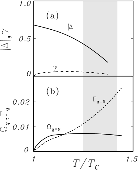
FIG. 10.: The evolution of the single particle parameters $\Delta_{\rm pg}$ and $\gamma$ (a), contrasted with the pair parameters $\Omega_{\bf q}$ and $\Gamma_{\bf q}$ (b). The coupling is fixed at $g/g_{c}=1.2$. For temperatures above and below the shaded area, the lowest order theory and mode coupling scheme are used, respectively. Curves inside the shaded region were obtained by interpolation.

FIG. 11.: Comparison of the $T_{c}$ curves within the BCS theory (dotted line), the Nozières–Schmitt-Rink scheme (dashed line), and our mode coupling results (heavy line). The inset shows the dependence of the chemical potential $\mu(T=T_{c},g)$ on the coupling constant for these three cases.

FIG. 12.: The evolution of $T_{c}$, $\mu$, and $|\Delta|$ with coupling strength in self-consistent mode coupling theory.

FIG. 13.: $T_{c}$ versus coupling constant over an extended range for three different values of the parameter $k_{\rm F}/k_{0}$. The minimum in the two larger $k_{0}$ curves is associated with $\mu=0$.

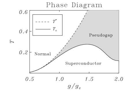
FIG. 14.: Quantitative phase diagram in the fermionic regime, $\mu>0$. The shaded region indicates where there is a well established pseudogap in the single particle spectral function.

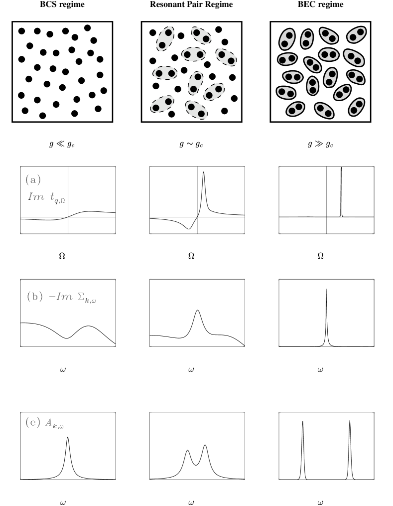
FIG. 15.: Summary of our conclusions: schematic plot of the resonant pair or pseudogap regime as a crossover between free fermions (BCS) and bound fermions (Bose-Einstein) with fermions indicated by the solid dots, dashed lines around pairs denote metastable pair states, while stable preformed pairs are represented by encircled pairs. Panels (a), (b) and (c) illustrate the evolution with coupling of: (a) ${\it Im}\,t_{{\bf q=0},\Omega}$, (b) $-{\it Im}\Sigma_{{\bf k},\omega}$, and (c) $A_{{\bf k},\omega}$. The vertical scales of figures for BCS and resonance regime have appeared elsewhere, throughout the paper.

- [1] D.C. Johnston, PRL 62, 957, (1989).
- [2] J. Rossat-Mignod et al, Physica B 169, 58(1991). J. Rossat-Mignod et al, Physica B 180-181, 383 (1992).
- [3] C. C. Homes et al., Phys. Rev. Lett. 71 1645 (1993); A. V. Puchkov et al.,J. Phys (Cond Matt) 8 10049 (1996).
- [4] H. Ding et al., Nature 382 51 (1996);
- [5] A. G. Loeser et al., Science 273 325 (1996).
- [6] P. A. Lee, N. Nagaosa, T. K. Ng and X.-G. Wen, Phys. Rev. B 57 6003 (1998) and references therein.
- [7] P. W. Anderson, The Theory of Superconductivity in the High-Tc Cuprate Superconductors (Princeton University Press, Princeton, 1997).
- [8] H. Fukuyama, Prog. Theor. Phys. Suppl. No. 108, 287 (1992). For recent developments see H. Fukuyama and H. Kohno J. Magn. Magn. Mater. 177, 483 (1998), Physica C 282 124 (1997), Czech. J. Phys. 46 3146, Suppl. 6 (1996) and references therein.
- [9] D. Pines, Physica C 282 273 (1997); Z. Phys. B 103 129 (1997) and references therein.
- [10] J. R. Schrieffer and A. P. Kampf, J. Phys. Chem. Sol. 56, 1673 (1995).
- [11] A. V. Chubukov et al., J. Phys. (Cond. Matt.) 8, 10017 (1996);
- [12] V. Emery, S. A. Kivelson, Phys. Rev. Lett. 74, 3253 (1995); Nature 374 434 (1995).
- [13] M. Randeria et al., Phys. Rev. Lett. 62, 981 (1989);
- [14] C. A. R. Sa de Melo, M. Randeria, and J. R. Engelbrecht, Phys. Rev. Lett. 71, 3202 (1993).
- [15] R. Micnas et al., Phys. Rev. B 52, 16 223 (1995).
- [16] J. Ranninger et al., Phys. Rev. B 53, R 11 961 (1996).
- [17] A. S. Alexandrov, Philos. T. Roy. Soc. A 356 197 (1998), and references therein.
- [18] T. D. Lee, Nature, 330 460 (1987), Phys. Scripta T42 62 (1992); R. Friedberg, T. D. Lee, C. Ren Phys. Rev. B 45, 10732 (1992);
- [19] O. Tchernyshyov, Phys. Rev. B 56, 3372 (1997).
- [20] Y. J. Uemura, Physica C 282 194-197 (1997).
- [21] V. B. Geshkenbein, L. B. Ioffe, A. I. Larkin, Phys. Rev 55, 3173 (1997).
- [22] B. Janko, J. Maly and K. Levin, Phys. Rev. B 56, R 11 407(1997).
- [23] The difficulty lies in the analytical continuation to the real axis of the Green’s function obtained numerically for a finite number of Matsubara frequencies. For a discussion of these and related issues see J. Schmalian et al., Comp. Phys. Commun. 93, 141 (1996).
- [24] J. Maly, B. Janko, and K. Levin, (cond-mat/9710187, submitted to Phys. Rev. B).
- [25] see J. Maly, K. Levin, and D.Z. Liu, Phys. Rev. B 54, 15657 (1996).
- [26] A. J. Leggett, J. Phys. (Paris) 41, C7 (1980).
- [27] The need for self-consistently finding the chemical potential in the context of the BCS-BEC crossover was first suggested by D. M. Eagles, Phys. Rev. 186, 456 (1969).
- [28] P. Nozières and S. Schmitt-Rink, J. Low Temp. Phys. 59, 195 (1985).
- [29] N. Trivedi, and M. Randeria, Phys. Rev. Lett. 75, 312 (1995); J. M. Singer, M. H. Pedersen, T. Schneider, Physica B 230 955 (1997); Phys. Rev B 54 1286 (1996).
- [30] B. L. Gyorffy, J. B. Staunton, G. M. Stocks, Phys. Rev. B. 44, 5190 (1991). E. V. Gorbar, V. M. Loktev, S.G. Sharapov Physica C 257 355 (1996); V. P. Gusynin, V. M. Loktev, S.G. Sharapov JETP Lett. 65 182 (1997); M. Marini, F. Pistolesi, and G. C. Strinati, Eur. Phys. J. B 1, 151 (1998).
- [31] L.P. Kadanoff and P. C. Martin, Phys. Rev. 124, 670 (1961). Reference 13 in this paper is particularly pertinent here; A. Klein, Nuovo Cimento 25, 788 (1962).
- [32] B. R. Patton, PhD Thesis, Cornell University, 1971 (unpublished); Phys. Rev. Lett 27, 1237 (1971).
- [33] The detailed form used here for the T-matrix is more readily related to that in Ref. [32] than in Ref.[31].
- [34] I. Kosztin et al., (to be published).
- [35] R. Haussmann, Phys. Rev. B 49, 12975 (1994).
- [36] J. M. Serene, Phys. Rev. B. 40, 10873 (1989).
- [37] J. J. Deisz, D. W. Hess and J. W. Serene, Phys. Rev. Lett. 80, 373 (1998).
- [38] J. R. Engelbrecht, A. Nazarenko, M. Randeria, E. Dagotto (preprint, cond-mat/9705166).
- [39] M. Letz and R. J. Gooding, (cond-mat/9802107); G. Esirgen and N. E. Bickers Phys. Rev. B 57 5376 (1998); S. Grabowski, J. Schmalian, K. H. Bennemann Physica C 282-287 1775 (1997); T. Dahm Solid State Commun. 101 487 (1997); M. Y. Kagan , R. Fresard, M. Capezzali, H. Beck Phys. Rev. B 57 5995 (1998). M. H. Pedersen, J. J. Rodriguez-Nunez, H. Beck, T. Schneider, S. Schafroth, Z. Phys. B 103 21 (1997).
- [40] Q. Chen, et al. (preprint, cond-mat/9805032).
- [41] It should also be noted that we have verified that this diagrammatic scheme is consistent with the general criteria for number conservation in G. Baym and L. P. Kadanoff, Phys. Rev. 124, 287 (1961). Other conservation laws are also satisfied. For the energy conservation see V. Ambegaokar and G. Rickayzen, Phys. Rev. 142, 146 (1966).
- [42] G. Baym, Phys. Rev. 127, 1391 (1962).
- [43] H. J. Vidberg and J. W. Serene, J. Low Temp. Phys. 29, 179 (1977).
- [44] For convenience, the solid line in Figure 5 also corresponds to a small expansion. Detailed numerical studies indicate that the small approximation is extremely good.
- [45] Here we have dropped a structureless term which may be parameterized as . This is relatively unimportant near and in the well developed pseudogap regime. It will play a role near when the cross-over to Fermi liquid behavior occurs. Moreover, its presence is necessary to ”regularize” the self energy when is arbitrarily small so that self energy is never a strict delta function in the normal state.
- [46] S. L. Cooper and K. E. Gray, in Physical Properties of High Temperature Superconductors IV, Chapter 3, p. 61, Edited by D. M. Ginsberg (World Scientific, London, 1994).
- [47] W. F. Brinkman and S. Engelsberg, Phys. Rev. 169, 417 (1968).
- [48] Y. M. Vilk et al. (preprint, cond- mat/9710013). Y. M. Vilk and A. M. S. Tremblay, J. Phys I (France) 7, 1309 (1997). Y. M. Vilk, C. Liang, A. M. S. Tremblay Phys. Rev. B, 49, 13267 (1994).
- [49] M. Drechsler and W. Zwerger, Ann. Physik 1, 15 (1992);
- [50] S. Schmitt Rink, C. M. Varma, A. E. Ruckenstein, Phys. Rev. Lett. 63, 445 (1989).
- [51] A. Tokumitu, K. Miyake, K. Yamada, Physica B 165-166 1039 (1990); Prog.. Theor. Phys. Suppl. No. 106, 63 (1991); Phys. Rev. B, 47 11988, (1993).
- [52] S. Marcelja, Phys. Rev. B 1, 2531 (1970).
- [53] A. Schmid, Z. Phys. 231, 324 (1970). It is interesting to note that within this lowest order approximation, the difference between the FLEX scheme employed here and the asymmetric choice of Marcelja (preceeding reference) is the well-known factor of 2 difference in the two–particle self energy. See also A. Schmid, Z. Phys. 229, 81 (1969). This discrepancy, on the other hand, is already enough to spoil the agreement with the BCS result when extended to .
- [54] Figure 1(c) elucidates the connection of the present work to earlier “mode-coupling” schemes of Marcelja and Yamada: By iterating this equation, we find that the so-called “box-approximation” for two–particle self–energy, employed by Schmid, Marcelja and Yamada and collaborators (see text), corresponds to the first, , term in the infinite series of polygon self-energy diagrams with vertices (“2n–gon”-s), fully accounted for in the present self-consistent scheme.
- [55] K. Levin and O. T. Valls, Phys. Rev. B 17 191 (1978); A. Zawadowski, K. Penc and G. T. Zimanyi, Prog. Theor. Phys. Suppl. No. 106, 11 (1991); K. Penc and A. Zawadowski, Phys. Rev. B 50, 10 578 (1994). We thank A. Zawadowski for drawing our attention to these results.
- [56] M. R. Norman, M. Randeria, H. Ding, and J. C. Campuzano (preprint, cond-mat/9711232)