The analysis of single crystal diffuse scattering using the Reverse Monte Carlo method: Advantages and problems

Abstract

The scattering from crystals can be divided into two parts: Bragg scattering and diffuse scattering. The analysis of Bragg diffraction data gives only information about the average structure of the crystal. The interpretation of diffuse scattering is in general a more difficult task. A recent approach of analysing diffuse scattering is based on the Reverse Monte Carlo (RMC) technique. This method minimises the difference between observed and calculated diffuse scattering and leads to one real space structure consistent with the observed diffuse scattering.

The first example given in this paper demonstrates the viability of the RMC methods by refining diffuse scattering data from simulated structures showing known occupational and displacement disorder. As a second example, results of RMC refinements of the diffuse neutron- and X-ray scattering of stabilised zirconia (CSZ) are presented. Finally a discussion of the RMC method and an outlook on further developments of this method is given.

I Introduction

Crystal structure analysis based on Bragg diffraction data reveals only information about the average crystal structure, such as atomic positions, thermal ellipsoids and site occupancies. Any departure from the strictly long-range-ordered average structure of the crystal gives rise to diffuse scattering containing information about static or thermal disorder within the studied material. Since many properties like optical properties, hardness, ionic conductivity are governed by structural disorder, the determination of the defect structure based on diffuse scattering data can reveal important information about the studied material. The development of area detectors (proportional counters, image plates, CCD) in recent years has enormously increased the capability for measuring generally weak diffuse neutron and X-ray scattering data. However, the interpretation and analysis of diffuse scattering remains a generally difficult task. The availability of modern (super)computers opens a wide area of computer simulation techniques to aid the analysis of diffuse scattering. An overview of traditional approaches and the analysis of diffuse scattering via computer simulations can be found in [1], further general information about disorder diffuse scattering can be found in numerous review articles [2, 3, 4, 5, 6, 7]. We want to focus in this paper on the analysis of diffuse single crystal scattering using the RMC method developed by McGreevy and Pusztai [8].

The RMC refinement technique minimises the difference between observed and calculated diffuse scattering intensities as a function of the positions and occupancies of the atomic sites in the model crystal. Although the RMC method is known for about 10 years, the application of RMC to diffuse single crystal scattering data was reported just recently in a neutron diffraction study of the diffuse scattering of ice Ih [9]. The advantage of the RMC method is the fact, that it is a model free method to analyse diffuse scattering, i.e. no assumptions about the particular disordered structure under investigation have to be made. In general a RMC simulation gives one real-space structure consistent with the experimental data. The remaining difficulty is the interpretation of the resulting structure.

The aim of this paper is to give an introduction into the RMC simulation technique for the analysis of diffuse single crystal scattering and to discuss the advantages and difficulties of the RMC method.

II The RMC method

In general Monte Carlo methods can be described as statistical simulation methods involving sequences of random numbers to perform the simulation. In the past several decades this simulation technique based on the algorithm developed by Metropolis [10] has been used to solve complex problems in nuclear physics, quantum physics, chemistry as well as for simulations of e.g. traffic flow or econometrics. The name Monte Carlo was coined during the Manhattan Project in World War II, because of the similarity of statistical simulation to games of chance, and because the capital of Monaco was a center of gambling. In this analogy the ’game’ is a physical system and the scientist might ’win’ a solution for his particular problem. An excellent application for this kind of statistical method is the study of diffuse scattering and subsequently the solution of the underlying defect structure. One possible approach is the (direct) Monte Carlo (MC) modeling of a defect structure from a given set of near-neighbour interaction energies [1]. The same basic algorithm is used for RMC simulations to minimise the difference between calculated and measured diffuse scattering as described in the following section.

A How does it work ?

As described in the introduction, the aim of the RMC simulation process is to minimise the difference between observed and calculated diffraction pattern. As a first step, the scattered intensity is calculated from the chosen crystal starting configuration and a goodness-of-fit parameter $\chi^{2}$ is computed.

$$\chi^{2}=\sum_{i=1}^{N}\frac{(I_{e}({\bf h}_{i})-I_{c}({\bf h}_{i}))^{2}}{\sigma^{2}}$$ (1)

The sum is over all measured data points ${\bf h}_{i}$, $I_{e}$ stands for the experimental and $I_{c}$ for the calculated intensity. The RMC simulation proceeds with the selection of a random site within the crystal. The system variables associated with this site, such as occupancy or displacement, are changed by a random amount, and then the scattered intensity and the goodness-of-fit parameter $\chi^{2}$ are recalculated. The change $\Delta\chi^{2}$ of the goodness-of-fit $\chi^{2}$ before and after the generated move is computed. Every move which improves the fit ($\Delta\chi^{2}<0$) is accepted. ’Bad’ moves worsening the agreement between observed and calculated intensity are accepted with a probability of $P=\exp(-\Delta\chi^{2}/2)$. As the value of $\Delta\chi^{2}$ is proportional to $1/\sigma^{2}$, the value of $\sigma$ has an influence on the amount of ’bad’ moves which will be accepted. Obviously there are two extremes: For very large values of $\sigma$, the experimental data are ignored ($\chi^{2}\approx 0$) and with very small values of $\sigma$ the fit ends up in the local minimum closest to the starting point, because there is a negligible probability for ’bad’ moves. The parameter $\sigma$ acts like the temperature $T$ in ’normal’ MC simulations. The RMC process is repeated until $\chi^{2}$ converges to its minimum.

The result of a successful RMC refinement is one real space structure which is consistent with the observed diffuse scattering data. In order to exclude chemically implausible resulting structures additional constrains, e.g. minimal allowed distances between atoms, may be introduced.

B RMC software

FIG. 1.: Illustration of the different RMC modes: (a) swap atoms, (b) shift atom and (c) swap displacements from average position.

The program used for the RMC refinements presented in this paper is DISCUS [11]. For practical use it is necessary to include a scaling factor $f$ and a background parameter $b$ in the previous definition of the goodness-of-fit $\chi^{2}$. A weight $w({\bf h})$ is included as well. DISCUS allows the user to choose a particular weighting scheme or read weights from a separate input file. The definition of $\chi^{2}$ becomes:

$$\chi^{2}=\sum_{i=1}^{N}\frac{w({\bf h}_{i})[I_{e}({\bf h}_{i})-(f\cdot I_{c}({\bf h}_{i})+b)]^{2}}{\sigma^{2}}$$ (2)

As before $I_{e}({\bf h}_{i})$ stands for the measured intensity at the reciprocal point ${\bf h}_{i}$, and $I_{c}({\bf h}_{i})$ is the calculated intensity in that point. The summation is over all N experimental data points. Three different ways to calculate the scale $f$ and background $b$ are implemented. First the user can define fixed values for both: $f=f_{0},b=b_{0}$. Secondly, the background can be set to a fixed value $b=b_{0}$ and the scaling factor $f$ is computed according to:

$$f=\frac{\sum\limits_{i=1}^{N}w({\bf h}_{i})I_{e}({\bf h}_{i})I_{c}({\bf h}_{i})-b_{0}\sum\limits_{i=1}^{N}w({\bf h}_{i})I_{c}({\bf h}_{i})}{\sum\limits_{i=1}^{N}w({\bf h}_{i})I_{c}^{2}({\bf h}_{i})}$$ (3)

Alternatively both values $f$ and $b$ can be refined during the RMC refinement. Equation (5) shows the corresponding definitions.

$$f = \frac{\sum\limits_{i=1}^{N}w({\bf h}_{i})\sum\limits_{i=1}^{N}w({\bf h}_{i})I_{e}({\bf h}_{i})I_{c}({\bf h}_{i})-\sum\limits_{i=1}^{N}w({\bf h}_{i})I_{e}({\bf h}_{i})\sum\limits_{i=1}^{N}w({\bf h}_{i})I_{c}({\bf h}_{i})}{\sum\limits_{i=1}^{N}w({\bf h}_{i})\sum\limits_{i=1}^{N}w({\bf h}_{i})I_{c}^{2}({\bf h}_{i})-\left(\sum\limits_{i=1}^{N}w({\bf h}_{i})I_{c}({\bf h}_{i})\right)^{2}}$$ (4)

$$b = \frac{\sum\limits_{i=1}^{N}w({\bf h}_{i})I_{e}({\bf h}_{i})-f\cdot\sum\limits_{i=1}^{N}w({\bf h}_{i})I_{c}({\bf h}_{i})}{\sum\limits_{i=1}^{N}w({\bf h}_{i})}$$ (5)

The parameters $f$ and $b$ are computed in each RMC cycle and have usually large starting values as long as there are big differences between calculated and observed data. After every RMC move the resulting scattering intensity and the $\chi^{2}$ value is calculated. In order to save computing time only the contribution of the modified atoms to the scattering is calculated. The difference $\Delta\chi^{2}=\chi_{old}^{2}-\chi_{new}^{2}$ is taken to decide if the move will be accepted or not as described in the previous section. The program calculates separate scaling factors and background parameters for every used plane of experimental data.

The program DISCUS is capable of modeling occupational as well as displacement disorder and so far we have called each crystal modification simply RMC move. In practice we use a mode (’switch-atoms’) of simulation in which occupational disorder is modeled by swapping two different randomly selected atoms (Fig. 1). This procedure forces the relative abundances of the different atoms within the crystal to be constant. It should be noted, that vacancies are treated as an additional atom type within the program DISCUS. The introduction of displacement disorder is realised in two different ways. In the first method a randomly selected atom is displaced by a random Gaussian distributed amount (’shift’, Fig. 1b). Alternatively the displacement variables associated with two different randomly selected atoms are interchanged (’switch-displacements’, Fig. 1c). The latter method has the advantage that the overall mean-square displacement averages for each atom site can be introduced into the starting model and these will remain constant throughout the simulation. Additional information about the program DISCUS can be found on the World-Wide-Web [13].

III Examples

A RMC test refinements

In this first example, we test the viability of the RMC simulation technique for systems showing occupational and displacement disorder in combination. First a disordered structure with given correlation parameters and displacements is created and the diffuse intensity calculated. This intensity is used as input for the RMC refinement. Finally the resulting structure is compared to the expected disordered structure. Details about the complete series of test simulations can be found in [12].

	Input		Run A		Run B		Run C
$c_{10}$	-0.	203	0.	188	-0.	076	-0.	124
$c_{11}$	0.	523	0.	290	0.	412	0.	465
$d_{zr-zr}$ [Å]	5.	05(12)	5.	02(9)	5.	02(8)	5.	03(6)
$d_{zr-vac}$[Å]	4.	89(9)	4.	95(11)	4.	97(10)	4.	94(10)
$R$	-		39.	3 %	39.	2 %	7.	7 %

TABLE I.: Input structure and results of RMC test refinements

The simulated structure used to calculate the ’experimental’ data for the RMC refinements was a 2D square-symmetric crystal with a size of 50x50 unit cells, one atom (Zr) at (0,0,0) with an occupancy of 0.83 and a lattice constant of a=5Å. We chose the defect ’test’ structure to consist of preferred vacancy pairs in $<$11$>$ direction and a subsequent relaxation of the surrounding atoms towards the vacancy. The vacancy ordering can be described using the correlation coefficient $c_{ij}$ which is defined as:

$$c_{ij}=\frac{P_{ij}-\theta^{2}}{\theta(1-\theta)}$$ (6)

$P_{ij}$ is the joint probability that both sites $i$ and $j$ are occupied by the same atom type and $\theta$ is its overall occupancy. Negative values of $c_{ij}$ correspond to situations where the two sites $i$ and $j$ tend to be occupied by different atom types while positive values indicate that sites $i$ and $j$ tend to be occupied by the same atom type. A correlation value of zero describes a random distribution. The maximum negative value of $c_{ij}$ for a given concentration $\theta$ is $-\theta/(1-\theta)$ ($P_{ij}=0$), the maximum positive value is +1 ($P_{ij}=\theta$). We will refer to the correlation coefficient of nearest neighbours in $<$10$>$ direction as $c_{10}$ and in $<$11$>$ direction as $c_{11}$. The achieved vacancy concentration $\theta$ and correlation values $c_{10}$, $c_{11}$ are listed in Table I. The resulting structure is characterised by a positive correlation $c_{11}$ and a negative value for $c_{10}$ close to its maximum negative value of $-\theta/(1-\theta)=-0.205$. In other words, the vacancy ordering is given by preferred $<$11$>$ vacancy pairs and avoided $<$10$>$ pairs.

The simulated structure and the corresponding diffraction pattern are shown in Figure 2a and 2d, respectively. The scattering pattern was computed on a grid of 301x301 points for neutron scattering at a wavelength of 1Å.

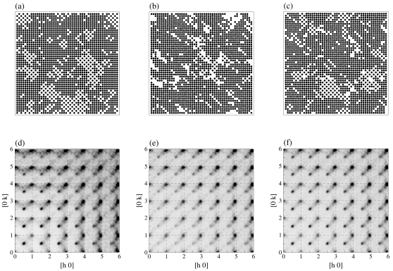
FIG. 2.: Input structure (a) for RMC test refinements showing preferred $<$11$>$ vacancy pairs and corresponding diffraction pattern (d). Resulting defect structure run A (b) and run B (c) and corresponding diffraction patterns (e) and (f).

The RMC simulations started from a structure showing a random vacancy distribution and displacements corresponding to an isotropic temperature factor of B=0.5 Ų. Simulation A was carried out by alternately executing one cycle in ’swap atoms’ mode followed by one cycle in ’swap displacements’ mode. A total of 15 cycles of each RMC mode was computed. In this paper a cycle will be the number of RMC moves necessary to visit each crystal site once on average. The resulting correlations, displacements and R-values are listed in Table I. The resulting final distortions are consistent with the expected size-effect like displacements, i.e. the atoms surrounding a vacancy are shifted towards the vacancy. The calculated diffraction pattern (Fig. 2e) shows a satisfactory agreement with the experimental data at high ${\bf Q}$ values, where as diffuse features at positions $(\frac{h}{2},\frac{k}{2})$, with $h$ and $k$ integer, at low ${\bf Q}$ are barely reproduced. These diffuse intensities are mainly caused by the vacancy ordering. The correlation values achieved (Tab. I) show positive values in the $<$10$>$ and $<$11$>$ directions rather than the expected negative correlation in $<$10$>$ direction. Consequently the resulting structure (Fig. 2b) shows a clustering of the vacancies rather than the expected vacancy ordering present in the model structure. It appears that the dominant part of the diffuse scattering caused by the displacements has a too strong an influence on the correlations that are achieved.

In order to model both parts of the defect structure more simultaneously, during run B the ’swap atoms’ and ’swap displacements’ modes were alternated every 0.1 cycles, i.e. the number of moves necessary to visit 10% of all atom sites on average. Additionally, the data set used for the ’swap atoms’ moves was limited to a range of $|{\bf Q}|<4.0$ r.l.u., i.e. only the low angle part, less affected by diffuse scattering due to distortions, was used to refine the vacancy ordering. The final values for the distortions (Tab. I) are similar to those of the previous run. However, visual inspection of the calculated diffraction patterns (Fig. 2f) shows a much better agreement, especially at low ${\bf Q}$ values, with the input data set compared to run A, although the R-value has only slightly improved. The resulting structure (Fig. 2c) and correlation values achieved (Tab. I) reflect the significantly improved description of the simulated disordered structure.

The simulation results presented here indicate that the RMC simulation technique is a powerful tool to analyse diffuse scattering and to obtain information about the defect structure even of quite complex systems showing both occupational and displacement disorder. However, the resulting correlation and displacement values are still significantly smaller than the expected values present in the input structure. Current efforts are to improve the results of RMC refinements by using a different way to calculate the diffuse diffraction pattern. Run C in Table I shows the results achieved using this modified technique. More details can be found in [14] and in the discussion of the RMC method in section IV A.

B Stabilised zirconia

The cubic phase of pure $ZrO_{2}$ is thermodynamically stable only at temperatures above 2370C. This phase, however, can be stabilised at room temperature by doping with oxides of a variety of lower valent metals, e.g. $CaO$, $MgO$, $Y_{2}O_{3}$. The average structure is of fluorite type, space group Fm3m, with zirconium on $(0,0,0)$ and oxygen on $(\frac{1}{4},\frac{1}{4},\frac{1}{4})$. The dopant cation occupies a zirconium site and in order to maintain charge neutrality, a corresponding number of oxygen vacancies is introduced resulting in important ceramic and ionic conduction properties of these materials. The diffuse scattering of these materials has been investigated by numerous workers (see references in [15, 16]. More recently, the authors of [17] described the diffuse X-ray and neutron scattering of Ca-CSZ ($Zr_{0.85}Ca_{0.15}O_{1.85}$) by a model of correlated microdomains using a formula for the diffuse intensity given by [18, 19]. The model consists of two types of microdomains, one based on a single vacancy with relaxed neighbouring atoms, the other based on a pair of vacancies separated by $\frac{1}{2}<$111$>$ over those oxygen cubes containing a metal atom. A quite different ’modulation wave’ approach to model the vacancy distribution by [20] provided further evidence for the existence of $\frac{1}{2}<$111$>$ vacancy pairs. A model for the diffuse scattering of yttrium stabilised zirconia (Y-CSZ) with a composition of $Zr_{0.61}Y_{0.39}O_{1.805}$ based on Monte Carlo (MC) simulations was given by [16, 21] Our most recent work on the diffuse scattering of CSZs [22] uses the RMC simulation technique to analyse the complex defect structure of these materials.

These RMC simulations of Ca-CSZ used neutron as well as X-ray diffuse scattering data as input. The X-ray data were collected on our PSD diffractometer system [23]. The neutron diffraction data used in this study were collected by [18]. A total of three layers of X-ray diffuse scattering, i.e. $0.3c^{*}$, $0.5c^{*}$ and $0.7c^{*}$, and two layers of neutron diffuse scattering, i.e. 0th and 2nd layer of [$1\overline{1}0$]-zone, were used as input for the RMC simulations (two layers are shown in Fig. 3a,b). Furthermore, the cubic symmetry of the crystal was taken into account assuming, that all symmetrically equivalent planes contain the same data as the experimental planes. This resulted in an effective number of data points in excess of 900000. The first RMC simulations were carried out using the largest computationally feasible crystal size of 20x20x20 unit cells containing a total of 96000 atoms (including vacancies). A total of 5 RMC cycles was carried out, giving a R-value of 29.6% (Run A). However, the resulting correlations (Tab. II) suggest that the good fit was mainly obtained by longer ranging correlations rather than the local disorder we are interested in.

Neighbour	Run A		Run B
Correlations
$VAC-VAC:\frac{1}{2}\langle 100\rangle$	-0.	005	-0.	008(11)
$VAC-VAC:\frac{1}{2}\langle 110\rangle$	-0.	014	-0.	011(10)
$VAC-VAC:\frac{1}{2}\langle 111\rangle^{*}$	0.	006	-0.	009(17)
$VAC-VAC:\frac{1}{2}\langle 111\rangle$	0.	008	0.	015(7)
$Ca-Ca:\frac{1}{2}\langle 110\rangle$	-0.	037	-0.	052(33)
$Ca-Ca:\langle 100\rangle$	-0.	009	-0.	008(17)
Displacements [Å]
$VAC-O:\frac{1}{2}\langle 100\rangle$	-0.	011	-0.	031(13)
$VAC-O:\frac{1}{2}\langle 110\rangle$	0.	003	0.	009(5)
$VAC-O:\frac{1}{2}\langle 111\rangle$	0.	005	0.	014(7)
$Zr-Zr:\frac{1}{2}\langle 110\rangle^{VAC}$	0.	024	0.	064(39)
$Zr-Zr:\frac{1}{2}\langle 110\rangle^{O}$	-0.	002	-0.	012(6)
$Zr-Ca:\frac{1}{2}\langle 110\rangle^{VAC}$	0.	020	0.	029(35)
$Zr-Ca:\frac{1}{2}\langle 110\rangle^{O}$	-0.	007	-0.	019(10)

TABLE II.: Results of the RMC refinements of the diffuse scattering of Ca-CSZ

In order to force the RMC process to model the diffuse scattering using correlations on a local scale, a series of RMC refinements, presented here, was carried out based on a crystal of only 5x5x5 unit cells in size. A total of 6 RMC refinements were computed (Run B), each run iterated for 25 cycles. The oxygen-oxygen vacancy ordering and the Zr-Ca ordering as well as displacements for all atoms were modeled. The simulation mode was similar to the one used for the test simulations described in the last section. The resulting average R-value for all refinements is 33.1%, the average of the resulting diffuse neutron and X-ray patterns of all RMC refinements are shown in Figure 3c and d, respectively.

Two different types of correlations are listed in Table II: The oxygen vacancy-vacancy correlations are represented by ’VAC-VAC’ and given for nearest neighbours ($\frac{1}{2}<$100$>$), next-nearest neighbours ($\frac{1}{2}<$110$>$) and second-nearest neighbours over those oxygen cubes containing no cation ($\frac{1}{2}<$111$>^{*}$) and those cubes filled with a cation ($\frac{1}{2}<$111$>$). Additionally the Ca-Ca occupancy correlations for nearest neighbours ($\frac{1}{2}<$110$>$) and next-nearest neighbours ($<$100$>$) are given. Inspection of Table II shows that the average of all RMC refinements using the 5x5x5 unit cell crystal (Run B) results in an oxygen-vacancy ordering scheme similar other models proposed in the literature. However, the given standard deviations indicate there is a large variation in the values obtained from the different RMC refinements, so that the actual values are barely significantly different from zero. The RMC run A using the 20x20x20 unit cell crystal shows the same general trends in the correlation values, although here magnitudes are generally even lower and in one case of opposite sign (VAC-VAC $\frac{1}{2}<$111$>^{*}$). Despite the actual values being small, the trends are quite definite and reproducible. It should be noted, that the larger values are obtained using a smaller crystal size, which is consistent with the view that the smaller system is less able to use long-range correlations to obtain the fit. The Ca-Ca correlations show negative values for nearest and next-nearest neighbours for both refinements, although again these are very low in magnitude. Such negative correlations indicate Ca-Ca nearest and next-nearest neighbours tend to be avoided, i.e. less probable than in a random cation distribution. Again the smaller model crystal size leads to slightly larger negative values.

The displacements listed in Table II are the distances from the average fluorite position. The results show that the nearest neighbour oxygens are shifted towards the vacancy along the $<$100$>$-direction whereas next-nearest and second-nearest neighbouring oxygen atoms are moved away from the vacancy. The metal-metal distance along $\frac{1}{2}<$110$>$ is shorter than in the average structure if both bridging oxygen sites are occupied. If one or both of these bridging sites is vacant, the metals are shifted further apart. The results listed in Table II show no significant difference for the displacements of Zr-Zr pairs compared to Zr-Ca pairs. As the correlation values, the refinement B shows the more significant values compared run A using the larger model crystal size. However, the large standard deviation of these displacements indicates large statistical errors due to the small crystal size. The resulting defect structure is consistent with previously reported models of the disorder in CSZ materials. These calculations as well as as well as a study of the diffuse scattering of $TlSbOGeO_{4}$ [24] have shown, that the size of the model crystal is determined by two conflicting requirements: a large crystal size gives sufficiently smooth diffraction patterns and statistically significant correlation parameters, but fit is obtained by many longer-range correlations rather than by few short-range correlations which are the parameters we are interested in. A small crystal size on the other hand reduces the number of variables and longer-range correlations but the calculated diffraction pattern is too noisy for a satisfactory fit and the resulting correlation values have large errors. Further discussion of this problem and a way to improve the RMC results is given in section IV A of this paper.

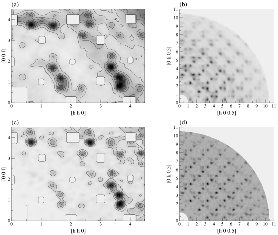
FIG. 3.: Diffuse scattering of Ca-CSZ: (a) neutron scattering of 0th layer of the [$1\overline{1}0$]-zone and (b) X-ray scattering of layer $0.5c^{*}$. Corresponding resulting diffraction patterns from RMC refinement: (c) neutron and (d) X-ray.

IV Discussion

Generally the RMC simulation technique generates a disordered structure consistent with the observed diffuse scattering by minimising the difference between calculated and measured diffuse scattering patterns. The RMC test simulations described here have demonstrated that the RMC technique is a viable tool to analyse diffuse scattering and to obtain information about the defect structure even for quite complex systems showing occupational and displacement disorder. The study of single crystal diffuse scattering of Ca-CSZ confirms that the RMC method is able to determine the characteristic features of the complex defect structure of a ’real’ disordered system. The combination of neutron and X-ray diffuse scattering data allowed the analysis to include oxygen-oxygen vacancy ordering as well as cation ordering and both oxygen and metal displacements. The resulting defect structure shows features consistent with results previously reported in the literature.

However, the resulting correlation parameters and displacements for the simulations of the diffuse scattering of Ca-CSZ were barely significantly different from zero although the trend towards the particular defect structure was reproducible. One important problem of the RMC simulation technique for single crystals is the size of the model crystal, determined by two conflicting requirements. This ’crystal size’ problem will be discussed in more detail in the next section.

A The ’crystal size problem’

RMC simulations of the diffuse scattering of CSZ presented here as well as a study of the diffuse scattering of $TlSbOGeO_{4}$ [24] have shown, that the size of the model crystal is determined by two conflicting requirements: a large crystal size gives sufficiently smooth diffraction patterns and statistically significant correlation parameters, but the fit is obtained by many longer-range correlations rather than by few short-range correlations which are the parameters we are interested in. A small crystal size on the other hand reduces the number of variables and longer-range correlations but the calculated diffraction pattern is too noisy for a satisfactory fit and the resulting correlation values have large errors.

One way to get around the described ’crystal size problem’ is the calculation of the diffuse scattering pattern as the average of intensities calculated from small regions (’lots’) within the model crystal chosen at random. This procedure results in a smooth diffraction pattern but, on the other hand, structural changes during the RMC refinement are done on a local scale within a single lot. Our current efforts are to incorporate this method of calculating smooth diffraction patterns by averaging the diffuse intensity of small areas within the crystal in the RMC refinement process. Additional to the high quality diffraction patterns obtained, this method results in a RMC refinement using only local correlations within one lot. First refinements of the diffuse scattering of the test structures [14] described in section III A of this paper using ’lots’ were carried out (Run C). Although the same disordered structure was used for these tests, the diffuse scattering used as ’experimental data’ for the RMC refinement was calculated using ’lots’ as well. Obviously the size of these ’lots’ must be large enough to contain all significant interactions. The resulting structure and diffraction pattern are shown in Figure 4a and 4b. Inspection of Table I shows for Run C correlations values and displacements significantly closer to the expected values present in the input structure. It should be noted, that the refinement using ’lots’ requires substantially more computer resources compared to ’normal’ RMC refinements. These test simulations demonstrate that the new RMC simulation technique using ’lots’ improves the resulting local disorder for the type of systems discussed in this paper.

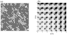
FIG. 4.: RMC refinement results from run C using ’lots’: (a) resulting structure and (b) corresponding diffraction pattern.

One might argue, that the desired restriction to a ’local’ scale in fact limits the potential of the RMC method. However, for many systems a ’local disorder’ model gives usually not only the simplest description of the particular disorder, but the local chemistry and near-neighbour interactions are frequently the interesting properties of the found defect structure. The test examples (see section III A) showing mainly short range order, were significantly better refined using the modified RMC simulation method using ’lots’ compared to the ’normal’ RMC refinement. One should bear in mind, that the RMC method produces the most disordered structure consistent with the data [9].

B What next ?

The RMC simulation technique has a large potential for further improvements and developments and, in the authors opinion, will continue to play its important role as method to analyse single crystal diffuse scattering.

Further developments of the RMC simulation technique to analyse diffuse scattering of single crystals are twofold: First constrains like minimal allowed distances between atom types can be used to avoid resulting structures which are unlikely or even impossible from a chemical of physical point of view. Those constrains can be highly specialised for a particular problem. A second major improvement can be expected from RMC simulations combining single crystal diffuse scattering data with other experimental data, e.g. powder diffraction data or EXAFS data. Thus a large RMC model could be constrained using experimental data more dependent on short range order. An the other hand unwanted long range fluctuations of might be suppressed by including Bragg data in the RMC refinement process. Besides the options already mentioned, one significant improvements would certainly be the possibility to used fully 3-dimensional data sets of diffuse scattering for the RMC refinement which is currently beyond available computer resources. With the continuing increase of available computing power, we will certainly see further developments in the area of computer simulations to aid the analysis of diffuse scattering in general and the RMC method in particular.

V Acknowledgments:

The RMC refinements of the diffuse scattering of CSZ were carried out on a Fujitsu VPP-300 supercomputer using a grant from the Australian National Supercomputer Facility. The work was supported in part by funds of the DFG (grant no. Pr 527/1-1).

REFERENCES

- [1] T.R. Welberry and B.D. Butler, J. Appl. Cryst. 27, 205 (1994)
- [2] T.R. Welberry, Rep. Prog. Phys. 48, 1543 (1985)
- [3] H. Jagodzinski, Prog. Cryst. Growth 14, 47 (1987)
- [4] H. Jagodzinski and F. Frey, International Tables for Crystallography, Chapter 4.2, 392 (1993)
- [5] F. Frey, Acta Cryst. B 51, 592 (1995)
- [6] F. Frey, Z. Kristallogr. 212, 257 (1997)
- [7] T.R. Welberry and B.D. Butler, Chem. Rev. 95, 2369 (1995)
- [8] R.L. McGreevy and L. Pusztai Mol. Simul. 1, 359 (1988)
- [9] V.M. Nield, D.A. Keen, and R.L. McGreevy, Acta Cryst. A 51, 763 (1995)
- [10] N. Metropolis, A.W. Rosenbluth, M.N Rosenbluth, A.H Teller, and E.J. Teller., J. Chem. Phys. 21, 1087 (1953)
- [11] Th. Proffen and R.B. Neder, J. Appl. Cryst. 30, 171 (1997)
- [12] Th. Proffen and T.R. Welberry, Acta Cryst. A 53, 202 (1997)
- [13] Th. Proffen and R.B. Neder, DISCUS WWW homepage, URL: http://www.pa.msu.edu/ proffen/discus/
- [14] Th. Proffen and T.R. Welberry, Z. Kristallogr. 212, 764 (1997)
- [15] Th. Proffen, R.B. Neder, F. Frey, and W. Assmus., Acta Cryst. B 49, 599 (1993)
- [16] T.R. Welberry, B.D. Butler, J.G. Thompson, and R.L. Withers, J. Solid State Chem. 106, 461 (1993)
- [17] Th. Proffen, R.B. Neder, and F. Frey, Acta Cryst. B 52, 59 (1996)
- [18] R.B. Neder, F. Frey, and H. Schulz, Acta Cryst. A 46, 792 (1990)
- [19] R.B. Neder, F. Frey, and H. Schulz, Acta Cryst. A 46, 799 (1990)
- [20] T.R. Welberry, R.L. Withers, and S.C. Mayo, J. Solid State Chem. 115, 43 (1995)
- [21] T.R. Welberry, R.L. Withers, J.G. Thompson and B.D. Butler, J. Solid State Chem. 100, 71 (1992)
- [22] Th. Proffen and T.R. Welberry, J. Appl. Cryst. 31, 318 (1998)
- [23] J.C. Osborn and T.R. Welberry, J. Appl. Cryst. 23, 476 (1990)
- [24] T.R. Welberry and Th. Proffen, J. Appl. Cryst. 31, 309 (1998)