Generalized Thermal Lattice Gases

Abstract

We show how to employ thermal lattice gas models to describe non-equilibrium phenomena. This is achieved by relaxing the restrictions of the usual micro-canonical ensemble for these models via the introduction of thermal “demons” in the style of Creutz. Within the Lattice Boltzmann approximation, we then derive general expressions for the usual transport coefficients of such models, in terms of the derivatives of their equilibrium distribution functions. To illustrate potential applications, we choose a model obeying Maxwell-Boltzmann statistics, and simulate Rayleigh-Bénard convection with a forcing term and a temperature gradient, both of which are continuously variable.

]

I Introduction

Frisch, Hasslacher and Pomeau (FHP) [1, 2] pioneered the use of Lattice Gas Automata (LGA) to simulate the Navier-Stokes (NS) fluid. The motion of fictitious particles on an underlying hexagonal lattice, subject to carefully chosen rules for collisions and propagation, gives rise to the NS equations in the continuum limit. Since that time, the LGA model and its derivative, the Lattice Boltzmann (LB) model [3], have attracted considerable attention because of their potential application to the simulation of complex fluid systems, in particular, systems with inter-particle interactions which model phase transitions and the dynamics of interfaces. Although the earliest such models [4] achieved spatial variation of the order parameter only by ignoring even semi-detailed balance in the description of possible collisions, more recent models are free from such inconsistencies [5].

However, like the original FHP model, all these models are intrinsically “athermal” [6], and so are unable to simulate phenomena where the temperature is an important variable. Only recently have thermal LGA models been constructed, such that the thermodynamics of fluids can be studied [7, 8, 9, 10, 11], and, typically, they are defined within a micro-canonical ensemble. To satisfy strict conservation rules for particle number, momentum and energy, they must contain several species of particles with different energies, interacting via rules which are often very complex. Reference [8], for example, is an extension of the FHP model to $4$ species of particles with carefully chosen momenta and energies, and in references [9, 10], the authors have to introduce unequal masses for particles moving in different channels, in order to ensure a sufficient number of allowed collisions. Thermal LB models are in principle less complex because they are expressed in terms of the distribution functions for the fictitious particles, but have not been conspicuously successful [12].

A more serious problem for the study of thermal phenomena, particularly those of a non-equilibrium nature (heat conduction) or involving instabilities (convection), arises because both LGA and LB thermal models treat the temperature as an externally defined parameter. However, when the temperature is itself a spatially varying parameter, it is necessary to have information about its variation in order to implement the collision rules (LGA) or the relaxation process (LB). Consequently, when this spatial variation is itself the object of study, it is not possible without modification [13] to apply existing models.

Our purpose in this paper is to introduce a class of thermal models which permit the study of non-equilibrium phenomena. As a by-product, these models permit a much wider variety of collision rules for LGA models, and are also readily adapted to the LB approach. The key feature is a novel idea drawn from the Monte-Carlo literature [14, 15, 16]. In the language of the Ising model, each site is associated with a local thermal reservoir or “demon”, which interchanges energy with the particles on the site. The local thermodynamic temperature, in the low velocity limit, is then proportional to the local demon energy. In the LGA or LB models, each demon is associated with one node of the hexagonal lattice, and constitutes a mechanism for monitoring or controlling the local temperature, so that the modeling of non-equilibrium phenomena becomes possible.

In the following section, we describe the equilibrium properties of such thermal lattice gas models. Then, in Section III, we derive expressions for the transport coefficients of Lattice Boltzmann models by means of a Chapman-Enskog expansion. In Section IV, we illustrate ideas using a particular model, and in Section V, as a specific example, use this model to simulate two-dimensional Rayleigh-Bénard convection and to draw some preliminary conclusions concerning the feasibility of our approach.

II Thermal Lattice Gas Models

A Generalities

In analogy with the basic LGA model [2], we define a class of thermal models in which several species of fictitious particles move on a two-dimensional hexagonal lattice. Some of the particles (rest particles) remain at rest. During each time step, the particles interact (“collide” like billiard balls) and then propagate ballistically at constant speed from one site of the lattice to a neighbouring site. The collision step rigorously conserves the number of particles and their total momentum. Energy is also conserved, but in a particular manner, described below.

Energy is defined as the sum of the kinetic and potential energies of the individual fictitious particles, and it is essential that there be at least two species of particles with distinct energies for there to be well-defined thermal properties. In the literature, such thermal models often employ only kinetic energies, so that within the micro-canonical ensemble, particles with different speeds and or masses [8, 9, 10] are required to satisfy the conservation laws. (This restriction to kinetic energies and to collision processes which strictly conserve energy also has the consequence [17] that such models posses zero bulk viscosity.) However, the inclusion of potential energy terms is straightforward, [10, 7], although seldom employed for other than pedagogical purposes.

Conservation of energy is enforced with the aid of the so-called demons, one at each site. The advantage of this procedure is that it is not necessary to choose values of masses, speeds and/or energies to permit a sufficient number of non-trivial collisions. Instead, a demon acts as a kind of energy reservoir, permitting collisions in a manner which satisfies detailed balance. Over the course of time, there will be a distribution function for the local demon energy, which has the form $P(E_{D})\sim\exp{-\beta E_{D}}$, where $\beta=1/T$ is the inverse of the local temperature. Since $E_{D}$ is a continuously variable quantity, its average value $<\!E_{D}\!>$ is equal to the local temperature. The idea is borrowed from Creutz [14], and was exploited in a series of papers applying Ising-style lattice gas models to non-equilibrium interface problems [18].

At each site, a collision process may proceed either if it produces surplus (or zero) energy or if the local demon can provide the requisite energy deficit. In the former case, the demon absorbs the surplus. Demons are required always to have positive energy, and as a result serve also to regulate the occurrence of collision processes. As demonstrated by Creutz and by Jörgenson et al [18], the demons thus act as thermometers, measuring the local temperature by virtue of their own statistically averaged energy. It is also possible to use the demons to control the local temperature: if this is done at the boundaries of a sample, then, for example, a temperature gradient can be set up across the sample, permitting a measurement of thermal conductivity [19] or the establishing of Rayleigh-Bénard convection.

A useful way to understand the role of the demons is to consider them as a species of rest particle. Rest particles of the conventional kind can be created or annihilated in collision processes so as to satisfy the conservation laws. Demons are neither created nor annihilated, but act to satisfy the conservation of energy. Conventional rest-particles (usually) have only one energy level, but demons have many such levels - although in simple situations one might imagine demons with only a small number of distinct levels [16].

B Statistical Equilibrium

As a first step in deriving expressions for the transport coefficients we define some generic notation [2]. Sites in the hexagonal lattice are labeled by an index i and by a site vector ${\bf R}_{i}$. The vectors radiating from a site i to its (not-necessarily) nearest neighbours define different possible directions for the motion of fictitious particles at that site. For particles of species $I$, we have ${\bf c}_{a,I},~{}a=1,2,\cdots,b_{I}$, where $b_{I}$ is the number of distinct neighbours at distance $c_{I}$. This distance also defines the “speed” of the species $I$, so that the kinetic energy of each fictitious moving particle is $\frac{1}{2}c_{I}^{2}$. In similar fashion, each particle of species $I$ has potential energy $\epsilon_{I}$, so that its total energy is $E_{I}=\frac{1}{2}c_{I}^{2}+\epsilon_{I}$. Any rest particle has total energy zero.

The fictitious particles occupy the available states $\{i,a,I\}$ according to particular statistics, and the detailed balance property of the collision rules guarantees that the system possesses a state of statistical equilibrium. Furthermore, the existence of an equilibrium distribution function is an essential condition for the regaining of the Navier-Stokes equations in the continuum limit [2]. The usual choice of statistics is Fermi-Dirac, since, historically, it was convenient for coding purposes to represent occupation numbers as binary variables. However, this choice is not essential. In general we write the occupation number of the state $\{i,a,I\}$ as $n_{i,a,I}$, and the ensemble-averaged distribution function for this state as $f_{i,a,I}=<\!n_{i,a,I}\!>$. It is convenient to represent rest particles in the same way by $n_{i,0}$ and $f_{i,0}$.

In an equilibrium state for which there is no net motion of the fluid, the functions $f$ have the values $f^{eq}_{I}$, so that the probability of finding a certain configuration can then be written as a product of the continuous variables $f^{eq}$ and $P(E_{D})$, the latter variable being the probability of finding a demon with energy $E_{D}$. It is now possible to define thermodynamic variables in terms of the equilibrium distributions.

The most important of these are the density $\rho$ and the pressure, $P$. The density is just

$$\rho=Mf^{eq}_{0}+\sum_{a,I}f^{eq}_{I}\equiv\rho_{0}+\sum_{I}\rho_{I}$$ (1)

where $M$ is the number of rest-particle states per site. In principle, the pressure should be derived from the free energy. However, as is well known in the lattice gas literature [2, 6], the quantity which plays the role of pressure in the hydrodynamic equations is

$$P=\frac{1}{2}\sum_{I}c_{I}^{2}\rho_{I}$$ (2)

sometimes known as the “kinetic pressure”. It is useful to define the analogous partial pressures $P_{I}=\frac{1}{2}c_{I}^{2}\rho_{I}$, so that $P=\sum_{I}P_{I}$. We will also require the energy density $U=\sum_{I}E_{I}\rho_{I}$ [20], and the isothermal and adiabatic speeds of sound, which are respectively

$$c_{T}^{2}=\frac{1}{2}\sum_{I}\rho_{I}c_{I}^{2}/\rho$$ (3)

and

$$c_{s}^{2}=\frac{1}{2}\sum_{I}f^{\mu}_{I}c_{I}^{4}/\sum_{I}f^{\mu}_{I}c_{I}^{2}$$ (4)

The derivatives $f^{\mu}_{I}$ of the equilibrium distribution functions $f^{eq}_{I}$ are defined as $f^{\mu}_{I}=T\left(\frac{\partial f_{I}}{\partial\mu}\right)_{\!T}$ where $T$ is the temperature and $\mu$ is the chemical potential [21].

When there exists a net local flow velocity ${\bf u}$ it is still possible to define equilibrium distribution functions. In the low velocity limit $u\ll c$, they can be expanded in powers of ${\bf u}$. Following reference [2], but with a slightly generalised notation, we obtain to first order [22]

$$f^{eq}_{a,I}({\bf u})=f^{eq}_{I}+q\rho f^{\mu}_{I}{\bf c}_{a,I}\cdot{\bf u}$$ (5)

The constant $q$ is determined by requiring that the expansions be consistent with the total momentum defined as

$$\rho{\bf u}=\sum_{a,I}{\bf c}_{a,I}f^{eq}_{a,I}$$ (6)

We obtain

$$q=2/\sum_{I}b_{I}f^{\mu}_{I}c_{I}^{2}$$ (7)

(8)

and it is convenient to define $q_{I}=qf^{\mu}_{I}$ so that

$$f^{eq}_{a,I}({\bf u})=f^{eq}_{I}+\rho q_{I}{\bf c}_{a,I}\cdot{\bf u}$$ (9)

and $\frac{1}{2}\sum b_{I}q_{I}c_{I}^{2}=1$. Note that to first order in ${\bf u}$, there are no corrections to $f^{eq}_{0}$ or to $P(E_{D})$.

C Time Evolution

As in a traditional LGA [2], time evolution proceeds in two distinct steps. First, particles at a given site, (both rest particles and moving particles in any energy level), interact with each other (“collide”) following predetermined rules [2]. Energy conservation is ensured by the local demon, as described previously, and detailed balance is rigorously observed. Conservation of particles, momentum and energy on each site can be written explicitly as

$$\sum_{a,I}f_{i,a,I}(t)+f_{i,0}(t)={\textstyle constant}$$ (10)

$$\sum_{a,I}{\bf c}_{a}f_{i,a,I}(t)={\textstyle constant}$$ (11)

$$\sum_{a,I}f_{i,a,I}(t)E_{I}+E_{D,i}(t)={\textstyle constant}$$ (12)

where $t$ is the (discrete) time. $E_{D,i}$ is the demon energy.

After each collision step, there is a propagation step, in which each moving particle moves one lattice constant in the direction of its velocity, while the rest particles and the demon remain unchanged. Thus the kinetic equations for the particle and demon variables, including both collisions and propagation, are:

$$f_{j,a,I}(t+1)-f_{i,a,I}(t) = \Omega_{I},~{}~{}~{}a=1,\cdots,b_{I}$$ (13)

$$f_{i,0}(t+1)-f_{i,0}(t) = \Omega_{0},$$ (14)

$$E_{D,i}(t+1)-E_{D,i}(t) = -\sum_{I}\sum_{a}^{b_{I}}\Omega_{I}E_{I}$$ (15)

where the index $j$ is defined by ${\bf R}_{j}={\bf R}_{i}+\hat{\bf c_{a}}$. $\Omega$ is the ensemble averaged collision operator. Strictly speaking, $E_{D,i}$ should also be replaced by its ensemble average, $<\!E_{D,i}\!>$.

The lattice Boltzmann approximation to the collision matrix directly employs the existence of equilibrium distribution functions. Any distribution function which deviates from its equilibrium value can be written as $f=f^{eq}+g$, where $g$ is hopefully small. If we assume that there exists a single characteristic relaxation time $\tau$ [23], then in terms of $g$, we may approximate the rate equations as

$$f_{j,a,I}(t+1)-f_{i,a,I}(t) = -g_{i,a,I}/\tau,~{}~{}~{}a=1,\cdots,b_{I}$$ (16)

$$f_{i,0}(t+1)-f_{i,0}(t) = -g_{i,0}/\tau$$ (17)

These expressions will be employed to simplify the analysis in the subsequent parts of the paper.

III Transport Coefficients

The basic continuum equations for a thermal fluid could now be obtained via a Chapman-Enskog expansion. However, since such treatments are available elsewhere [10], we will focus only on the derivation of expressions for the transport coefficients. We will follow the procedure of reference [2]. The first step is to replace the rate equations (16), (17) by their continuum versions. In the limit where spatial and temporal changes are small and/or slow, the left-hand sides of these equations yield derivatives which can be replaced by $\partial_{t}=\epsilon\partial_{t_{1}}$ $+\epsilon^{2}\partial_{t_{2}}$, $\nabla{r}=\epsilon\nabla{r_{1}}$, where $\epsilon$ is a small parameter. The distribution functions can also be expanded in terms of $\epsilon$. To order $\epsilon^{2}$, this gives:

$\displaystyle f_{a,I}=f^{(0)}_{a,I}+\epsilon f^{(1)}_{a,I}+\epsilon^{2}f^{(2)}_{a,I},$

and

$\displaystyle f_{0,I}=f^{(0)}_{0,I}+\epsilon f^{(1)}_{0,I}+\epsilon^{2}f^{(2)}_{0,I}$

where the zeroth order terms in the expansion are just the equilibrium distributions, and the higher order terms are just $g$: $f^{eq}\equiv f^{(0)}$ and $g\equiv\epsilon f^{(1)}+\epsilon^{2}f^{(2)}$. Necessarily, the conservation of mass, momentum and energy require that

$$f^{(\alpha)}_{0}+\sum_{a,I}f^{(\alpha)}_{a,I}=0,$$ (18)

$$\sum_{a,I}{\bf c}_{a}f^{(\alpha)}_{a,I}=0$$ (19)

and

$$E_{D}^{(\alpha)}+\sum_{a,I}E_{I}f^{(\alpha)}_{a,I}=0$$ (20)

where $\alpha=1,2$.

Substituting into equations (16)-(17), and equating terms for each order of $\epsilon$, we obtain a hierarchy of Boltzmann equations. The first order equations are:

$$D^{(1)}_{a,I}f^{(0)}_{a,I}\equiv(\partial_{t_{1}}+{\bf c}_{a,I}\cdot\nabla_{1})f^{(0)}_{a,I}=-{1\over\tau}f^{(1)}_{a,I},$$ (21)

$$\partial_{t_{1}}f^{(0)}_{0}=-{1\over\tau}f^{(1)}_{0},$$ (22)

$$\partial_{t_{1}}E_{D}^{(0)}=-{1\over\tau}E_{D}^{(1)}.$$ (23)

Using (18) and (19) we then obtain

$$\partial_{t1}(\rho)+\nabla_{1}\cdot(\rho{\bf u})=0$$ (24)

and

$$\partial_{t1}(\rho{\bf u})+\nabla_{1}P=0$$ (25)

where $P$ is the kinetic pressure as defined earlier. Similarly, since these relations are true for any values of the distribution functions $f^{eq}({\bf u}=0)$, there must also be analogous relations for the partial densities $\rho_{I}$ and partial pressures $P_{I}$, namely

$$\partial_{t1}(\rho_{I})+\frac{\rho_{I}}{\rho}\nabla_{1}\cdot(\rho{\bf u})=0$$ (26)

and

$$\partial_{t1}(\rho_{I}{\bf u})+\nabla_{1}P_{I}=0$$ (27)

The expressions for the shear viscosity $\nu$, the bulk viscosity $\zeta$ and the thermal conduction coefficient $\lambda$ arise from the second order terms in $\epsilon$. After some reduction, the corresponding equations become

$$\partial_{t2}(\rho)+\frac{1}{2}\sum_{a,I}D^{(1)}_{a,I}D^{(1)}_{a,I}f^{(0)}_{a,I}=0$$ (28)

and

$$\partial_{t2}(\rho{\bf u}) + \frac{1}{2}\sum_{a,I}D^{(1)}_{a,I}D^{(1)}_{a,I}{\bf c_{a,I}}f^{(0)}_{a,I}$$ (29)

$$+ \sum_{a,I}{\bf c_{a,I}}{\bf c_{a,I}}\cdot\nabla_{1}f^{(1)}_{a,I}=0$$ (30)

where the terms preceded by the factor $\frac{1}{2}$ are second order in the Taylor expansion of the derivatives. These terms can be reduced by making use of the equations (18) and (21). Although equation (28) reduces to the simple result $\partial_{t2}(\rho)=0$, equation (30) is more interesting. We simplify its second term to read $\sum_{a,I}{\bf c_{a,I}}\cdot\nabla_{1}D^{(1)}_{a,I}{\bf c_{a,I}}f^{(0)}_{a,I}$, and then substitute for $f^{(1)}_{a,I}$ from (21) to obtain

$$\partial_{t2}\rho({\bf u})=(\tau-\frac{1}{2})\sum_{a,I}{\bf c}_{a,I}\cdot\nabla_{1}D^{(1)}_{a,I}{\bf c_{a,I}}f^{(0)}_{a,I}$$ (31)

The final step is to substitute (9), and use (26) and (27) to write

$$\partial_{t2}(\rho{\bf u})=(\tau-\frac{1}{2})\sum_{I}(X_{I}\nabla^{2}\rho{\bf u}+Y_{I}\nabla\nabla\cdot\rho{\bf u})$$ (32)

where

$\displaystyle X_{I}=\frac{1}{4}b_{I}q_{I}c_{I}^{4}$

and

$\displaystyle Y_{I}=\frac{1}{2}(b_{I}q_{I}c_{I}^{4}-\rho_{I}c_{I}^{2}/\rho)$

Combining with (25), this becomes

$$\partial_{t}(\rho{\bf u})=-\nabla P+(\tau-\frac{1}{2})(\nu\nabla^{2}\rho{\bf u}+\zeta\nabla\nabla\cdot\rho{\bf u})$$ (33)

where the shear viscosity $\nu$ is

$\displaystyle\nu=\frac{1}{2}c_{s}^{2}(\tau-\frac{1}{2})$

and the bulk viscosity $\zeta$ is

$\displaystyle\zeta=(c_{s}^{2}-c_{T}^{2})(\tau-\frac{1}{2})$

using the expressions for the sound speeds $c_{T}$ and $c_{s}$ given earlier. Note that the bulk viscosity vanishes for any model having only one value of the speeds $c_{I}$: this includes any FHP1 model, [2], as a special case.

The procedure to obtain the thermal conduction coefficient, $\lambda$, is very similar to that described, for example, in Huang [24]. A key feature is the necessity to subtract out of the energy current that part which depends on the net flow of the fluid. This is the origin of the “subtracted current” described by Ernst [7, 17], but neglected by Chen et al [10]. We account for this effect by replacing the energies $E_{I}$ by $\tilde{E}_{I}$ such that

$$\sum_{a,I}{\bf c}_{a,I}\tilde{E}_{I}f^{eq}_{a,I}({\bf u})=0$$ (34)

or

$$\sum_{I}b_{I}f_{I}^{\mu}c_{I}^{2}\tilde{E}_{I}=0$$ (35)

Writing $\tilde{E}_{I}=E_{I}-E_{S}$, we obtain

$$E_{S} = \sum_{I}b_{I}q_{I}E_{I}c_{I}^{2}/\sum_{I}b_{I}q_{I}c_{I}^{2}$$ (36)

$$= \sum_{I}b_{I}f^{\mu}_{I}E_{I}c_{I}^{2}/\sum_{I}b_{I}f^{\mu}_{I}c_{I}^{2}$$ (37)

The first order equation describing the time evolution of the local energy density $\tilde{U}=\sum_{a,I}f^{eq}_{a,I}({\bf u})\tilde{E}_{I}$ is then

$$\partial_{t1}[\tilde{U}+E_{D}]=0$$ (38)

which gives no new information. However, after using equations (20)-(21), the second order equation becomes

$$\partial_{t2}[\tilde{U}+E_{D}]=(\tau-\frac{1}{2})\sum_{a,I}\tilde{E}_{I}{\bf c}_{a,I}\cdot\nabla D^{(1)}_{I,a}f^{eq}_{I,a}({\bf u})$$ (39)

Using the explicit form of $f^{eq}_{I,a}({\bf u})$, equation (9), and the definition of $\tilde{E}$, equation (35), we therefore obtain

$$\partial_{t}[\tilde{U}+E_{D}]=(\tau-\frac{1}{2})\sum_{I}\tilde{E}_{I}c_{I}^{2}\nabla^{2}\rho_{I}$$ (40)

It remains to express the gradient explicitly in terms of the thermal gradient. In the absence of a net flow of particles, the chemical potential $\mu$ is not a function of position, and so $\nabla^{2}f_{I}=f_{I}^{T}\nabla^{2}T$, where $f_{I}^{T}=\left(\frac{\partial f_{I}}{\partial T}\right)_{\!\mu}$, and the coefficient of thermal conduction is

$$\lambda=(\tau-\frac{1}{2})\sum_{I}b_{I}f_{I}^{T}c_{I}^{2}\tilde{E}_{I}/2$$ (41)

It is convenient to write this also in the form

$$\lambda=(\tau-\frac{1}{2})\frac{1}{T^{2}}\sum_{I}b_{I}f_{I}^{\beta}c_{I}^{2}\tilde{E}_{I}/2$$ (42)

where $\beta=\frac{1}{T}$ and $f_{I}^{\beta}$ is given by $f_{I}^{\beta}=-\left(\frac{\partial f_{I}}{\partial\beta}\right)_{\!\mu}$. The high temperature behaviour of $\lambda$ is dominated by the $\frac{1}{T^{2}}$ prefactor.

For the particular case of the Fermi-Dirac distribution, it is easy to show that this is precisely the expression given by Ernst [17]. We write $f_{I}^{\beta}=-(\mu-E_{I})f_{I}^{\mu}$ and therefore obtain

$$\lambda = (\tau-\frac{1}{2})\frac{1}{T^{2}}\sum_{I}b_{I}f_{I}^{\mu}c_{I}^{2}\tilde{E}_{I}(E_{I}-\mu)/2$$ (43)

$$\equiv (\tau-\frac{1}{2})\frac{1}{T^{2}}\sum_{I}b_{I}f_{I}^{\mu}c_{I}^{2}\tilde{E}_{I}^{2}/2$$ (44)

where the last step comes from the identity (35).

IV A Model

To illustrate the ideas of the previous sections, and, in particular, to illustrate the use of statistics other than Fermi-Dirac, we have previously described a model where the statistics are quite unconventional [25]. In the present paper, we choose to employ Maxwell-Boltzmann statistics for a simple model with 3 energy levels. The lowest level, with energy $E_{0}=0$, is $M$-fold degenerate, so that there are at most $M$ fictitious particles with zero velocity (“rest particles”). The other two levels both correspond to the same speed $c$, with the same 6-fold symmetry as in the FHP models, but their energies are respectively $E_{A}$ and $E_{B}=E_{A}+\Delta$. In our numerical calculations, we take $E_{A}=0.62$ and $E_{B}=1.80$ in units of $c^{2}$.

Assuming Maxwell-Boltzmann statistics, we obtain

$\displaystyle f_{0}({\bf u})=e^{\beta\mu};\,\,\,f_{I,a}({\bf u})=e^{\beta(\mu-E_{I})}(1+q\rho{\bf u}\cdot c_{a}),\,\,\,I=A,B$

where $q=\rho e^{-\beta\mu}/3c^{2}(e^{-\beta E_{A}}+e^{-\beta E_{B}})$, and $\rho e^{-\beta\mu}=[M+6(e^{-\beta E_{A}}+e^{-\beta E_{B}})]$. This simple form for the velocity expansion results because $f_{I}^{\mu}=f_{I}^{eq}$.

Because there is only one speed in the model, the expressions for the sound velocities and for the shear and bulk viscosities become particularly simple. We obtain

$$c_{T}^{2} = \frac{1}{2}c^{2}\frac{\sum_{A,B}\rho_{I}}{\rho}=3c^{2}\left[\frac{e^{-\beta E_{A}}+e^{-\beta E_{B}}}{M+6(e^{-\beta E_{A}}+e^{-\beta E_{B}})}\right];$$ (45)

$$c_{s}^{2} = \frac{1}{2}c^{2}$$ (46)

and

$$\nu = (\tau-\frac{1}{2})c^{2}/4;$$ (47)

$$\zeta = (\tau-\frac{1}{2})\frac{c^{2}}{2}\frac{\rho_{0}}{\rho}$$ (48)

$$= (\tau-\frac{1}{2})\frac{c^{2}}{2}\frac{M}{M+6(e^{-\beta E_{A}}+e^{-\beta E_{B}})}$$ (49)

The temperature-independence of $\nu$ is an artifact of the model, but the temperature dependence of $\zeta$ is typical of the viscosity of a liquid. For a typical value of the density, $\zeta$ is displayed in Figure 1 as a function of temperature.

The model also leads to a simple expression for the thermal conduction coefficient $\lambda$:

$\displaystyle\lambda=(\tau-\frac{1}{2})\frac{3c^{2}\Delta^{2}}{T^{2}}\frac{f_{A}^{eq}f_{B}^{eq}}{f_{A}^{eq}+f_{B}^{eq}}$

For the purpose of illustration, it is convenient to relate this to the thermal diffusion coefficient, defined as $D_{T}=\lambda/\rho C_{p}$, which is also plotted in Figure 1. Although the temperature dependence of $\lambda$ is dominated by the $\frac{1}{T^{2}}$ prefactor at high temperatures, $T>\Delta$, this behaviour is exactly compensated by the temperature dependence of the specific heat.

FIG. 1.: Temperature variation of the transport coefficients for the model described in the text. Solid line: bulk viscosity. Dashed line: shear viscosity. Dotted line: thermal diffusion. Dash-dotted line: sound attenuation. All coefficients are in units of $\tau-\frac{1}{2}$.

For completeness, Figure 1 also shows the temperature variation of the sound attenuation coefficient $\Gamma$, defined in the standard way as $\Gamma=\frac{1}{2}(\nu+\zeta+(\gamma-1)D_{T})$.

V Rayleigh Bénard Convection

To illustrate the feasibility of our approach, we carried out simulations of Rayleigh-Bénard convection. We considered a two dimensional cell with horizontal length $L$ and vertical height $H$. Periodic boundary conditions were imposed in the horizontal direction, with two rigid walls at the top and the bottom of the cell. The demon energies on the upper and lower walls were fixed at values $T_{1}$ and $T_{2}$, respectively. A uniform force was implemented by changing the vertical momentum of the particles at a constant rate, while keeping horizontal momentum unchanged. Thus, both the temperature difference $\delta T$ and the force could be tuned continuously.

Our initial study was of a system with $L=400$ lattice units and $H=100\times\sqrt{3}$ units, so that the aspect ratio $L:H$ was near $2:1$, with a particle density of $3.6$ per site. The energy levels were $E_{A}=0.62$, $E_{B}=1.8$ in units of $c^{2}$, and the temperatures at the lower and upper boundaries were $T_{1}=4.8$, $T_{2}=0.3$ in the same units. We chose the relaxation time $\tau$ to be 1 unit, and averaged velocity fields over $20\times 20$ regions in order to evaluate the local distribution functions. Initial conditions were a uniform density and a uniform temperature gradient, and with the local velocity everywhere zero, so that we were able to observe the onset and subsequent evolution of the convective instability. With these parameters, the evolution of the system was sufficiently slow that “snapshots” of the velocity field could be obtained by time averages over only $50$ time-steps.

Figure 2 shows the evolution of the temperature distribution, and of the corresponding velocity fields for these parameters. At first four convection rolls are clearly seen, but subsequently these collapse into two. Evidently, the model has captured the essential features of the physical phenomenon. Systematic analysis of the data as a function of the system parameters will be the subject of a subsequent publication, but certain preliminary remarks are appropriate here.

According to the classic linear stability analysis, [26], convection occurs when the Rayleigh number $\cal{R}$ [27] exceeds a critical value of order $10^{3}$. Even for situations far from the linear regime, the value of $\cal{R}$ is a good indicator of the stability of the convective phenomenon. Thus, since $\cal{R}$ is of order $10^{5}$ for the simulation shown in the figure, the convection rolls should be extremely stable, as is indeed the case. Indeed, our results are strikingly similar to those of a previous detailed study [13], obtained with a modified LB model which represented the temperature as a “convected passive scalar field”.

An interesting feature of our results is the observation of four rolls before the final stable state with two rolls is reached. Linear analysis predicts two rolls (since the wavenumber of the instability should be around $\pi/H$ where $H$ is the height of the cell). Our tentative explanation is that the velocity field is first established near the lower (hot) boundary, so that the effective height of the cell is considerably smaller than $H$. We therefore expect the wavenumber of the instability to be larger than $\pi/H$, and the periodic boundary conditions select $\sim 2\pi/H$. (In principle, with different geometry, we might expect to see yet higher initial wavenumbers.) The study of this transient regime, and the subsequent stabilisation of the two rolls, will form part of our ongoing investigations.

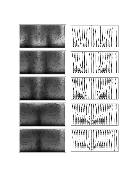
FIG. 2.: Contour plots showing the time evolution of the temperature distribution (left panels) and of the velocity field (right panels). From top to bottom, data is shown at times 20,000, 40,000, 60,000, 80,000 and 100,000 units respectively. One time unit is defined as one update of every site in the lattice.

However, in general terms, this preliminary illustration of Rayleigh-Bénard convection demonstrates the feasibility of our Lattice Boltzmann method for non-equilibrium thermal lattice-gases. We intend to apply our approach to a variety of phenomena for which the statistical mechanics of the gas are critically important. In particular, we plan to include interactions between fictitious particles so as to simulate systems with first order phase transitions and the dynamics of interfaces between their associated phases.

We thank Hong Guo and Martin Grant for many useful discussions.

REFERENCES

- [1] U. Frisch, B. Hasslacher, and Y. Pomeau, Phys. Rev. Lett. 56, 1505 (1986)
- [2] U. Frisch, D. d’Humières, B. Hasslacher, P. Lallemand, Y. Pomeau and J.-P. Rivet, Complex Systems 1, 649 (1987)
- [3] R. Benzi, S. Succi and M. Vergassola, Phys. Rep. 222, 145 (1992); F.J. Higuera, S. Succi and R. Benzi, Europhys. Lett. 9, 345 (1989)
- [4] D.H. Rothman and S. Zaleski, Rev. Mod. Phys. 66, 1417 (1994); D.H. Rothman and J. Keller, J. Stat. Phys. 52, 1119 (1988); C. Appert and S. Zaleski, Phys. Rev. Lett. 64, 1 (1990)
- [5] M.R. Swift, W.R. Osborn and J.M. Yeomans, Phys. Rev. Lett. 75, 830 (1995); M.R. Swift, E. Orlandini, W.R. Osborn and J.M. Yeomans, Phys. Rev. E 54, 5041 (1996); G. Gonella, E. Orlandini and J.M. Yeomans, Phys. Rev. Lett. 78, 1695 (1997)
- [6] M.H. Ernst, in Microscopic Simulations of Complex Hydrodynamical Processes, edited by M. Mareschal and B. Holian, (Plenum, New York, 1992)
- [7] M.H. Ernst and S.P. Das, J. Stat. Phys. 66, 465 (1992)
- [8] P. Grosfils, J.-P. Boon and P. Lallemand, Phys. Rev. Lett. 68, 1077 (1991); P. Grosfils, J.-P. Boon, R. Brito and M.H. Ernst, Phys. Rev. E, 48, 2655 (1993)
- [9] H. Chen, S. Chen, G.D. Doolen, Y.C. Lee and H.A. Rose, Phys. Rev. A 40, 2950 (1989)
- [10] S. Chen, H. Chen, G.D. Doolen, S. Gutman and M. Lee, J. Stat. Phys. 62, 1121 (1991)
- [11] X.W. Shan and H. Chen, Phys. Rev. E 47, 1815 (1993); X.W. Shan and H. Chen, Phys. Rev. E 49, 2941 (1994); X.W. Shan and G. Doolen, J. Stat. Phys. 81, 379 (1995)
- [12] F.J. Alexander, S. Chen and J.D. Sterling, Phys. Rev. E 47, 2249 (1993); Y. Chen, H. Ohashi and M. Akiyama, Phys. Fluids 7, 2280 (1995); G.R. McNamara, A.L. Garcia and B.J. Alder, J. Stat. Phys., 81 395 (1995)
- [13] X.W. Shan, Phys. Rev. E 55, 2780 (1997)
- [14] M. Creutz, Phys. Rev. Lett. 50, 1411 (1984)
- [15] G. Bhanot, M. Creutz and H. Neuberger, Nuc. Phys. B 235, 417 (1984)
- [16] M. Creutz, Ann. Phys. 167, 62 (1986)
- [17] M.H. Ernst, in Fundamental Problems in Statistical Mechanic, VII, edited by H. van Beijeren (Elsevier, Amsterdam, 1990)
- [18] R. Harris, L. Jörgenson, and M. Grant, Phys. Rev. A 45, 1024 (1992); R. Harris and M. Grant, J. Phys. A, 23, L567, (1990); L. Jörgenson, R. Harris and M. Grant, Phys. Rev. Lett. 63, 1693 (1989)
- [19] R. Harris and M. Grant, Phys. Rev. B 38, 9323 (1988)
- [20] Strictly speaking, the energy per unit area (rather than per site) requires an additional factor of . This same factor would appear in the expressions for the thermal conductivity and for the specific heats.
- [21] This is not the definition employed in reference [2], although the change in the algebra is minimal. The reason for the change is that it is useful to introduce the thermodynamic variables appropriate to thermal LGA models [17]. Because the volume of the system is by definition fixed, it is the density which provides the link with continuum models. This suggests that the notation of the grand canonical ensemble is the most appropriate, so that we will employ the temperature and the chemical potential .
- [22] The second order terms in the expansion have been omitted. It is well known, (see, for example, H. Chen, S. Chen, and W.H. Matthaeus, Phys. Rev. A 45, R5339 (1992) and references therein), that these terms give rise to important “corrections” to hydrodynamics, but such corrections are not our concern in this article. We plan to return to them on a future occasion.
- [23] P.L. Bhatnagar, E.P. Gross and M. Krook, Phys. Rev. 94, 511 (1954); Y.H. Qian, D. d’Humières and P. Lallemand, Europhys. Lett. 17, 479 (1992)
- [24] K. Huang, Statistical Mechanics, (Wiley, New York, 1987)
- [25] O. Baran, C.C. Wan and R. Harris, Physica A 239,322 (1997)
- [26] S. Chandrashekhar, Hydrodynamic and Hydromagnetic Stability, (Dover, New York, 1981)
- [27] The Rayleigh number is conventionally defined as , where is the thermal expansion coefficient, is the gravitational field, is the height of the cell, and is the temperature difference between the two boundaries.