Phase-Coherent Transport through a Mesoscopic System: A New Probe of Non-Fermi-Liquid Behavior

Michael R. Geller
Abstract

A novel chiral interferometer is proposed that allows for a direct measurement of the phase of the transmission coefficient for transport through a variety of mesoscopic structures in a strong magnetic field. The effects of electron-electron interaction on this phase is investigated with the use of finite-size bosonization techniques combined with perturbation theory resummation. New non-Fermi-liquid phenomena are predicted in the fractional quantum Hall effect regime that may be used to distinguish experimentally between Luttinger and Fermi liquids.

PACS: 73.20.Dx, 03.80.+r, 73.40.Hm

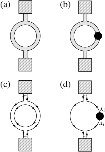
Resistance measurements have long been used as a spectroscopy of mesoscopic systems, as have other spectroscopies such as optical absorption. For example, a measurement of the tunneling current through a quantum dot as a function of temperature, voltage, and magnetic field, yields information about the electronic many-body states present there. Unfortunately, important information is lost in conventional tunneling spectroscopy because only the amplitude $|t|$ of the complex-valued transmission coefficient $t=|t|e^{i\phi}$ is measured. In a recent series of beautiful experiments, Yacoby et al. [1], Buks et al. [2], and Schuster et al. [3] have succeeded in measuring both the phase and amplitude of the transmission coefficient for tunneling through a quantum dot. The phase was measured by inserting a quantum dot into one arm of a mesoscopic interferometer ring and observing the shift in the Aharonov-Bohm (AB) magnetoconductance oscillations, thereby converting a phase measurement to a multi-probe conductance measurement. The experiments done in weak magnetic field used a ring-shaped semiconductor interferometer as shown schematically in Fig.ย 1a. AB oscillations in the conductance occur as the flux $\Phi$ enclosed by the ring varies. In Fig.ย 1b a phase-coherent scatterer with transmission coefficient $t=|t|e^{i\phi}$ is inserted into one arm of the interferometer, resulting in a shift of the phase of the magnetoconductance oscillations.

The properties of a ring interferometer in a strong magnetic field are strikingly different than that in weak field because of the formation of edge states. Under conditions in which the quantum Hall effect is observed, namely, when the Fermi energy in the bulk of the sample is in a mobility gap, the extended states responsible for transport lie at the device boundaries [4]. A bare interferometer in the quantum Hall regime is shown schematically in Fig.ย 1c. The source and drain contacts, denoted by the hatched regions, are assumed to be completely phase decoherent. Even in the absence of inserted scatterers, the chirality of the edge states dramatically changes the nature of the underlying AB interference: First, if there is no coherent transport between the left and right outer edge states, there will be no magnetoconductance oscillations at all, because the electrons will travel from source to drain without circling flux [5]. Therefore, weak phase-coherent tunneling points are introduced in Fig.ย 1c (denoted by dashed lines) to make a viable interferometer, although in a real system the coherence length in the contacts might be large enough to observe oscillations. Second, in a chiral system the AB oscillations are caused by interference between the direct path from source to drain along one edge of the ring and paths containing any number of windings around the ring having a given chirality. Whereas in the weak-field case the AB effect leads to both constructive and destructive interference (poles and zeros in the probability to propagate around the ring), the AB effect in a chiral system therefore leads to constructive interference (poles) only [6].

We are now in a position to understand the effect of inserting a mesoscopic phase-coherent scatterer, such as a quantum point contact or a quantum dot, into one arm of the strong-field interferometer. Elastic scattering between the inner and outer edge states is now possible, coupling them together in a phase-coherent fashion. Because the coupling to the inner edge state occurs in one arm only, electrons scattered to the inner edge state must eventually return to the outer edge state of that same arm. Therefore, the effect of any inserted scatterers is to introduce an equivalent scatterer with transmission coefficient $t$, shown as a black circle in Fig.ย 1d. Usually, $t$ results from the transmission through an inserted mesoscopic structure in parallel with the inner edge state of the ring. Comparing the equivalent circuits (b) and (d) in Fig.ย 1, we see that they are distinguished by the chiral nature of the latter. I shall therefore refer to the strong-field ring as a chiral interferometer. An immediate consequence of the chirality is that current conservation requires $t$ in case (d) to be a pure phase $e^{i\phi}$.

The purpose of this paper is to present a brief summary of the rich physics of the chiral interferometer. The model I shall adopt here for the interferometer is as follows: Two mesoscopic filling factor $g=1/q$ (with $q$ an odd integer) edge states are coupled to source and drain contacts. Weak phase-coherent tunneling points with reflection coefficient $\Gamma_{\rm c}$ (with $|\Gamma_{\rm c}|\ll 1$) couple the left and right edge states near the contacts to mimic the residual coherence necessary for strong-field interferometry, as discussed above. Because these couplings are assumed to occur in the contacts, the coefficients $\Gamma_{c}$ are assumed not to be renormalized by electron-electron interactions. The edges of the two-dimensional electron gas are assumed to be sharply confined, and the interaction short-ranged, so that the low lying collective excitations consist of a single branch of edge-magnetoplasmons with linear dispersion $\omega=vk$. Then the conductance at zero temperature is simply $G=g\big{(}1-2|\Gamma_{\rm c}|^{2}[1+\cos(\theta_{\rm out}+\phi)]\big{)}{e^{2}\over h},$ where $\theta_{\rm out}$ is the field-dependent phase accumulated by an electron after traversing the outer edge state. I have chosen this model for the bare interferometer because it is the simplest one that allows for a measurement of the phase $\phi$; more sophisticated models, including ones where $\Gamma_{\rm c}$ is renormalized by interactions, have been studied in a different context elsewhere [6, 7].

The dynamics of edge states in the fractional quantum Hall effect regime is governed by Wenโ€™s chiral Luttinger liquid (CLL) theory [8]

$$S_{\pm}={1\over 4\pi g}\int_{0}^{L}\!\!dx\int_{0}^{\beta}\!\!d\tau\ \partial_{x}\phi_{\pm}\big{(}\pm i\partial_{\tau}\phi_{\pm}+v\partial_{x}\phi_{\pm}\big{)},$$ (1)

where $\rho_{\pm}=\pm\partial_{x}\phi_{\pm}/2\pi$ is the charge density fluctuation for right (+) or left (โ€“) moving electrons. Canonical quantization in momentum space is achieved by decomposing the chiral scalar field $\phi_{\pm}$ into a nonzero-mode contribution $\phi_{\pm}^{\rm p}$ satisfying periodic boundary conditions, and a zero-mode part $\phi_{\pm}^{0}$. Imposing periodic boundary conditions on the bosonized electron field $\psi_{\pm}(x)\equiv(2\pi a)^{-{1\over 2}}e^{iq\phi_{\pm}(x)}e^{\pm iq\pi x/L}$ ($a$ is a microscopic cutoff length) leads to the requirement that the charge $N_{\pm}\equiv\int_{0}^{L}dx\ \rho_{\pm}$ be an integer multiple of $g$.

The study of mesoscopic effects in the CLL requires a careful treatment of the zero-mode dynamics. I shall make extensive use here of the retarded electron propagator Gยฑโ€‹(x,t)โ‰กโˆ’iโ€‹ฮ˜โ€‹(t)โ€‹โŸจ{ฯˆยฑโ€‹(x,t),ฯˆยฑโ€ โ€‹(0)}โŸฉsubscript๐บplus-or-minus๐‘ฅ๐‘ก๐‘–ฮ˜๐‘กdelimited-โŸจโŸฉsubscript๐œ“plus-or-minus๐‘ฅ๐‘กsuperscriptsubscript๐œ“plus-or-minusโ€ 0G_{\pm}(x,t)\equiv-i\Theta(t)\langle\{\psi_{\pm}(x,t),\psi_{\pm}^{\dagger}(0)\}\rangle for the finite-size CLL. In the presence of an AB flux $\Phi=\varphi\ \!\Phi_{0}$ (with $\Phi_{0}\equiv hc/e$) and additional charging energy $U$, the grand-canonical zero-mode Hamiltonian corresponding to (1) is $H^{0}_{\pm}={1\over 2}q\Delta\epsilon\big{(}N_{\pm}\pm g\varphi)^{2}+{1\over 2}UN_{\pm}^{2}-\mu N_{\pm},$ where $\Delta\epsilon\equiv 2\pi v/L$. I then obtain $\phi_{\pm}^{0}(x,t)=\pm 2\pi N_{\pm}(x\mp vt)/L-g\ \!\chi_{\pm}+g(\mu\mp\varphi\Delta\epsilon)t-gUN_{\pm}t,$ where $[\chi_{\pm},N_{\pm}]=i,$ and (at $T=0$)

$$G_{\pm}(x,t)=\pm\big{(}{\textstyle{i\over L}}\big{)}^{q}\ \!(\pi a)^{q-1}\ \!\Theta(t)\ \!e^{\pm iq\pi(x\mp vt)/L}\ \!e^{i(\mu\mp\varphi\Delta\epsilon)t}\big{\langle}e^{\pm 2\pi iqN(x\mp vt)/L}\ \!e^{-iUNt}\big{\rangle}\ {\rm Im}\ \!\bigg{(}{e^{-iUt/2}\over\sin^{q}\pi(x\mp vt\pm ia)/L}\bigg{)}.$$ (2)

The Fourier transform $G_{\pm}(x,\omega)$ is particularly interesting: For the case $U=0$, it is simply related to the Greenโ€™s function for noninteracting ($q=1$) chiral electrons [9],

$$G_{\pm}(x,\omega)=G_{\pm}^{q=1}(x,\omega)\times{\epsilon_{\rm F}^{1-q}\over(q-1)!}\prod_{j=1}^{q-1}\big{(}\omega-\omega_{j}\big{)}.$$ (3)

Here $\omega_{j}\equiv[j+{\rm frac}({\mu\over\Delta\epsilon}\mp\varphi)]\ \!\Delta\epsilon$, where ${\rm frac}(x)$ is the difference between $x$ and its closest integer, and $\epsilon_{\rm F}\equiv v/a$ is an effective Fermi energy. Whereas in the $q=1$ case the propagator has poles at each of the $\omega_{j}$, in the interacting case the first $q-1$ poles (above $\mu$) are removed. This effect, which can be regarded as a remnant of the Coulomb blockade for particles with short-range interaction, is a consequence of the factor $q$ in the first term of the zero-mode Hamiltonian $H_{\pm}^{0}$. Unlike an ordinary Coulomb blockade, however, the energy gap here, equal to $(q-1)\Delta\epsilon$, is exactly quantized. At higher frequencies or in the large $L$ limit where $\omega\gg\Delta\epsilon,$ the additional factor becomes $\omega^{q-1}/(q-1)!\ \!\epsilon_{\rm F}^{q-1}$. Upon turning on $U$ a conventional Coulomb blockade develops, with a gap given by $U+(q-1)\Delta\epsilon$.

The transmission coefficient for the equivalent scatterer in Fig.ย 1d can be shown to be given by the ratio of retarded propagators $t(\epsilon)\equiv G(x_{\rm f},x_{\rm i},\epsilon)/G_{\rm bare}(x_{\rm f},x_{\rm i},\epsilon),$ with $G_{\rm bare}$ referring to the bare interferometer, which is the appropriate generalization of the Fisher-Lee result [10] to this interacting system. The proof involves deriving an expression for the source-drain conductance of the interferometer with an arbitrary inserted scatterer, and extracting the phase shift caused by the latter. For the purpose of calculating $t$ we may neglect finite-size effects in the leads and assume $G_{\rm bare}(x_{\rm f},x_{\rm i},\epsilon)=G_{\rm bare}(d,\epsilon),$ where $d$ is the size of the inserted scatterer. I turn now to a summary of transmission coefficients for the configurations shown in Fig.ย 2; details of the calculations shall be given elsewhere.

(A) Single weak tunneling point.โ€”I begin with the simple case of one weak tunneling point at $x=x_{0}$ connecting the inner and outer edge states as shown schematically in Fig.ย 2A. In the fractional regime, quasiparticle tunneling, which is allowed in this configuration, diverges at low temperature, driving the system to the configuration shown in Fig.ย 2B [11]. In the integer regime $S=S_{0}+\delta S$, where $S_{0}=S_{\rm in}+S_{\rm out}$ is the sum of actions of the form (1) for the inner and outer edge states, respectively, and $\delta S=\int_{0}^{\beta}d\tau\ \![v\Gamma\psi_{\rm out}(x_{0},\tau){\bar{\psi}}_{\rm in}(x_{0},\tau)+{\rm c.c.}]$ is the weak coupling between them. To leading nontrivial order perturbation theory yields $t=1+v^{2}|\Gamma|^{2}G_{\rm in}(0,\epsilon)G_{\rm out}(a,\epsilon)$, where $d$ has been taken to be of the order of $a$. The Greenโ€™s function $G_{\rm in}(x,\omega)$ diverges at resonances associated with the inner edge state, invalidating low-order perturbation theory. However, it is possible to sum the perturbation expansion to all orders, resulting in

$$t={1+v^{2}|\Gamma|^{2}G_{\rm in}(0,\epsilon)\big{[}G_{\rm out}(a,\epsilon)-G_{\rm out}(0,\epsilon)\big{]}\over 1-v^{2}|\Gamma|^{2}G_{\rm in}(0,\epsilon)G_{\rm out}(0,\epsilon)}.$$ (4)

Note that in the CLL it is necessary to distinguish between $G_{\pm}(a,\epsilon)$ and $G_{\pm}(0,\epsilon)$, because $G_{\pm}(x,\omega)$ is proportional to the unit step function $\Theta(\pm x)$. At zero-temperature (and $U=0$) a simple expression for the phase shift in this configuration is possible, namely $\tan\phi=-{\textstyle{1\over 2}}|\Gamma|^{2}{\rm cot}(\theta_{\rm in}/2)\ \![1-{1\over 16}|\Gamma|^{4}\ {\rm cot}^{2}(\theta_{\rm in}/2)]^{-1},$ where $\theta_{\rm in}$ is the phase accumulated by an electron after circling the inner edge state [12].

(B) Single strong tunneling point.โ€”Next I consider the strong coupling limit of a single quantum-point-contact, as shown in Fig.ย 2B. In this case there is no quasiparticle tunneling. The interferometer is described by a single CLL, $S_{0}=S_{+}$, taken to be right-moving, and $\delta S=\int_{0}^{\beta}d\tau\ \![v\Gamma\psi_{+}(x_{1},\tau){\bar{\psi}}_{+}(x_{2},\tau)+{\rm c.c.}]$. Perturbation theory yields

$$t={G_{+}(L_{\rm in},\epsilon)-v\Gamma\ \!G_{+}(a,\epsilon)^{2}-v\Gamma^{*}\ \!G_{+}(L_{\rm in},\epsilon)^{2}\over G_{+}(d,\epsilon)},$$ (5)

and, at zero temperature (and $U$ = 0),

$$\tan\phi=\big{[}1+2\Gamma(\epsilon/\epsilon_{\rm F})^{q-1}{\rm csc}\ \!(\theta_{\rm in})/(q-1)!\big{]}\tan\theta_{\rm in},$$ (6)

where $L_{\rm in}$ is the length of the inner edge state. [For simplicity I have assumed in Eqn.ย (6) that $\Gamma$ is real and that $d$ is again of the order of $a$.] This expression shows that for $\Gamma=0$, $\phi$ varies linearly with $\epsilon/\epsilon_{\rm in}$ ($\epsilon_{\rm in}\equiv 2\pi v/L_{\rm in}$) with slope $2\pi$; for finite $\Gamma$ the phase oscillates about this linear variation as shown in Fig.ย 3.

(C) Two weak tunneling points.โ€”This configuration is similar to that in case A, and to leading order

$$t=1+v^{2}\big{(}\sum_{i}|\Gamma_{i}|^{2}\big{)}\ \!G_{\rm in}(0,\epsilon)G_{\rm out}(a,\epsilon)+v^{2}\Gamma_{1}\Gamma_{2}^{*}\ \!{G_{\rm in}(L_{\rm in}\!-d,\epsilon)\ \!G_{\rm out}(a,\epsilon)^{2}\over G_{\rm out}(d,\epsilon)}+v^{2}\Gamma_{1}^{*}\Gamma_{2}\ \!G_{\rm out}(d,\epsilon)\ \!G_{\rm in}(d,\epsilon),$$ (7)

where $d$ is now the distance between the two quantum point contacts.

(D) Quantum dot.โ€”Finally I consider the case of tunneling through a quantum dot weakly coupled to the interferometer edge states, as shown in Fig.ย 2D. In this configuration quasiparticle tunneling is not allowed, but Coulomb blockade effects are important in the quantum dot. The interferometer is described by $S_{0}=S_{+}+S_{\rm D}$, where $S_{\rm D}$ is the CLL action for the edge state in the quantum dot that includes an additional charging energy $U$, and the weak coupling of the quantum dot to the leads is described by $\delta S=\sum_{i}\int_{0}^{\beta}d\tau\ \![v\Gamma_{i}\psi_{+}(x_{i},\tau){\bar{\psi}}_{\rm D}(x_{i},\tau)+{\rm c.c.}]$, with $i=1,2.$ To leading nontrivial order (suppressing the $\epsilon$ dependence of the Greenโ€™s functions),

$$t={G_{+}(L_{\rm in})\over G_{+}(d)}+v^{2}\big{(}\sum_{i}|\Gamma_{i}|^{2}\big{)}\ \!{G_{\rm+}(a)\ \!G_{+}(L_{\rm in})\ \!G_{\rm D}(0)\over G_{+}(d)}+v^{2}\Gamma_{1}\Gamma_{2}^{*}\ \!{G_{+}(a)^{2}\ \!G_{\rm D}(L_{\rm D}/2)\over G_{+}(d)}+v^{2}\Gamma_{1}^{*}\Gamma_{2}\ \!{G_{+}(L_{\rm in})^{2}\ \!G_{\rm D}(L_{\rm D}/2)\over G_{+}(d)},$$ (8)

where $L_{\rm D}$ is the circumference of the quantum dot edge state. The first term in (8) describes transmission via the inner edge state; the order $|\Gamma_{i}|^{2}$ contributions describe the same, apart from an additional tunneling event on and back off the quantum dot at point $x_{i}$. The term proportional to $\Gamma_{1}\Gamma_{2}^{*}$ describes a direct tunneling through the dot, and the order $\Gamma_{1}^{*}\Gamma_{2}$ term describes transmission via the inner edge state, then backwards through the quantum dot, and finally around the inner edge state again. The propagator $G_{\rm D}(x,\omega)$ diverges at the quantum dot resonances, invalidating (8), and it is again necessary to sum the perturbation expansion to all orders; the result (for equal $\Gamma_{i}$) is

$$t={G_{+}(L_{\rm in})+v^{2}|\Gamma|^{2}\big{[}G_{+}(a)^{2}\ \!G_{\rm D}(L_{\rm D}/2)+2\ \!\Delta\ \!G_{+}(L_{\rm in})\ \!G_{\rm D}(0)\big{]}+v^{4}|\Gamma|^{4}\ \!\Delta^{2}\ \!G_{+}(L_{\rm in})\ \!\big{[}G_{\rm D}(0)^{2}-G_{\rm D}(L_{\rm D}/2)^{2}\big{]}\over G_{+}(d)\big{\{}1-v^{2}|\Gamma|^{2}\ \!\big{[}2\ \!G_{+}(0)\ \!G_{\rm D}(0)+G_{+}(L_{\rm in})\ \!G_{\rm D}(L_{\rm D}/2)]+v^{4}|\Gamma|^{4}\ \!G_{+}(0)^{2}\big{[}G_{\rm D}(0)^{2}-G_{\rm D}(L_{\rm D}/2)^{2}\big{]}\big{\}}},$$ (9)

where $\Delta\equiv G_{+}(a,\epsilon)-G_{+}(0,\epsilon).$ The energy-dependent phase for typical quantum dot parameters is shown in Fig.ย 3.

The non-Fermi-liquid nature of the transmission coefficient $t(\epsilon)$ in each configuration manifests itself as follows: At a fixed energy $\epsilon$, the phase shift $\phi$ as a function of magnetic field is the same as in a Fermi liquid ($q=1$), but the effective coupling constants depend on $\epsilon$. However, the energy dependence of $t(\epsilon)$ at fixed field (see Fig.ย 3), which can be probed by varying the temperature or bias voltage, is dramatically different than in the Fermi liquid case.

It is a pleasure to thank Hiroshi Akera, Eyal Buks, Zachary Ha, Jung Hoon Han, Jari Kinaret, Paul Lammert, Daniel Loss, Charles Marcus, Andy Sachrajda, Amir Yacoby, and Ulrich Zรผlicke for useful discussions.

REFERENCES

  • [1] A. Yacoby et al., Phys. Rev. Lett. 74, 4047 (1995).
  • [2] E. Buks et al., Phys. Rev. Lett. 77, 4664 (1996).
  • [3] R. Schuster et al., Nature 385, 417 (1997).
  • [4] B. I. Halperin, Phys. Rev. B 25, 2185 (1982).
  • [5] J. K. Jain, Phys. Rev. Lett. 60, 2074 (1988).
  • [6] M. R. Geller and D. Loss, Phys. Rev. B 56, 9692 (1997).
  • [7] C. de C. Chamon et al., Phys. Rev. B 55, 2331 (1997).
  • [8] X. G. Wen, Adv. Phys. 44, 405 (1995).
  • [9] M. R. Geller and D. Loss (unpublished).
  • [10] D. S. Fisher and P. A. Lee, Phys. Rev. B 23, 6851 (1981).
  • [11] C. L. Kane and M. P. A. Fisher, Phys. Rev. B 46, 15233 (1992).
  • [12] The phase subjected to an electron of energy $\epsilon$ after an orbit in the $\pm$ direction is $\theta_{\pm}(\epsilon)\equiv\oint{\bf p}\cdot d{\bf l}$. I take the single-particle dispersion to be $\pm v(k+2\pi\varphi/L)$, which leads to $\theta_{\pm}(\epsilon)=2\pi[(\epsilon/\Delta\epsilon)\mp\varphi]$.
Refer to caption
FIG.โ€„1.: (a) Semiconductor interferometer in zero field. A two-dimensional electron gas (shaded region) is connected to source and drain contacts. (b) Phase-coherent scatterer (solid black circle) with transmission coefficient $t$ inserted into one arm. (c) Interferometer in the quantum Hall effect regime, where edge states (solid lines) are formed. The dashed lines represent weak tunneling points. With no scatterers inserted the inner edge state is disconnected from the outer one and does not affect transport properties. (d) General configuration of the interferometer in the strong field case. The solid black circle denotes the transmission coefficient $t$ resulting from a coupling to the inner edge state caused by the insertion of an arbitrary phase-coherent scatterer. By unitarity, $t$ is a pure phase. Comparing cases (b) and (d) suggests the designation โ€œchiral interferometerโ€ for the latter.
Refer to caption
FIG.โ€„2.: Four configurations of the chiral interferometer: (A) One weak tunneling point connecting the inner and outer edge states. (B) One strong tunneling point. (C) Two weak tunneling points. (D) A quantum dot weakly connected to the incident edge states.
Refer to caption
FIG.โ€„3.: Phase of the transmission coefficient as a function of energy for configurations B and D. Here $\Delta\phi\equiv\phi-2\pi\epsilon/\epsilon_{\rm in}$, with $\epsilon_{\rm in}\equiv 2\pi v/L_{\rm in}$. The thin curves show the case $q=1$ and the thick ones $q=3$. The phase in configuration D is similar to that in B except for abrupt shifts caused by the quantum dot resonances; in the $q=3$ case the lowest resonances are blocked by interactions [see discussion following Eqn.ย (3)].