Kinetics of phase ordering on curved surfaces

Oliver Schoenborn and Rashmi C. Desai

   An interface description and numerical simulations of model A kinetics are used for the first time to investigate the intra-surface kinetics of phase ordering on corrugated surfaces. Geometrical dynamical equations are derived for the domain interfaces. The dynamics is shown to depend strongly on the local Gaussian curvature of the surface, and can be fundamentally different from that in flat systems: dynamical scaling breaks down despite the persistence of the dominant interfacial undulation mode; growth laws are slower than $t^{1/2}$ and even logarithmic; a new very-late-stage regime appears characterized by extremely slow interface motion; finally, the zero-temperature fixed point no longer exists, leading to metastable states. Criteria for the existence of the latter are derived and discussed in the context of more complex systems.    Key words: numerical simulations, interface description, kinetics, phase ordering, relaxation, dynamical scaling, model A, curved surface, lipid bilayer, dominant length scale

1 Introduction

Many two-dimensional surfaces exhibit internal degrees of freedom which allow for phase ordering or phase separation to occur within the static or dynamic surface. Examples are lipid bilayer membranes[1], crystal growth on curved surfaces[2], and thin film deposition[3]. Interaction between the shape and internal degrees of freedom of the surface are believed to play an important role in such systems, initiating, modifying or eliminating chemical or physical intra-membrane domain-ordering processes. The dynamics can be induced not only by varying the temperature, but also by changing such variables as the pH or ionic concentration of an aqueous embedding solution (in the case of lipid bilayers), or the lattice mismatch and deposition rate (film growth). Experimentally[4], both spinodal decomposition in binary mixtures and phase ordering in one-component systems have been observed. Phase ordering is more relevant to non-fluid phases and, in the case of biological lipid membranes, is possibly involved in the control of enzyme adsorption and protein-enzyme interaction on the surface of a bilayer.

For curved surfaces, the consequences of the interplay between surface shape and intra-surface pattern formation are at present largely unexplored in literature. The small amount of experimental results are rudimentary, and most of the theoretical work has been limited, due to the mathematical and numerical challenges involved, to equilibrium models and shape-perturbation calculations around equilibrium. Many of the theories assume that the domains are already formed (see, for instance, [5]). Typically, some form of bilinear coupling between an intra-membrane order parameter and the local geometry of the surface, such as mean curvature, is used. When kinetics are considered, one obtains a dynamical equation of state similar to that of the Random-Field Ising model with long-range correlations[6], but with the long-range correlations entering through the gradients of the intra-surface order-parameter[7]. One result has been the creation of shape phase-diagrams[1, 8]. Recently, some researchers have done simulations to investigate shape change in surfaces made of two types of lipids[9, 10]. These simulations, relying on Monte Carlo and bulk Langevin equations, are extremely computer intensive, limiting the possible complexity of the surfaces or the run time of the simulations to experimentally irrelevant cases.

Any dynamics occurring in curved spaces invariably introduces new and non-trivial concepts and effects which require considerable care and exploration. The problem of how the dynamical shape of a surface and an intra-membrane ordering process may affect each other is complicated. We therefore first consider the simplest case where there is no explicit coupling between the two, and new correlations arise through the geometry of the curved surface. Thus, rather than inquiring about the shape-change when the membrane is inhomogeneous, we investigate the influence of non-euclidean geometry on pattern formation and phase ordering kinetics when it occurs on a static curved surface. By comparing the results with known results for model A kinetics within a flat (euclidean) surface, we identify the sole effects arising from surface curvature. We hope that this will subsequently allow for a systematic extension of the problem in which the surface is not static and the explicit coupling between the intra-membrane order parameter and the local geometry of the surface is also included.

More explicitly, we report in this paper novel results of a ground-up study of relaxational pattern-formation occurring within static two-dimensional surfaces, using model A[11] as a starting point, without any explicit coupling to the local geometry other than through diffusion[7]. In section 2, we setup the analytical framework for the intra-surface phase ordering kinetics on curved surfaces. The bulk kinetics are described by the Non Euclidean Model A equation, Eq.(1). Systems with phase ordering instabilities, with homogeneous initial state and small random fluctuations, often evolve to form domains separated by sharp interfaces. The bulk part of the domains equilibrates rapidly and the interface width saturates within a very short time. Further time evolution involves only interface dynamics in which interfacial widths hardly change, but the total interfacial length decreases in order to minimise the system free energy. In order to take advantage of this type of kinetics, we deduce in section 2, a set of equations [Eqs. (2), (13) and (28)], which are equivalent to the bulk Non Euclidean Model A Eq.(1). In this interface description, local geodesic curvature of the interface, local velocity of the interface and total interfacial length $L(t)$ play a central role. One of the novel quantities that we investigate in detail in this paper (apparently for the first time in literature) is the Geodesic Curvature Autocorrelation Function. Equation (2) is the generalization of the well-known Allen-Cahn equation for intra-surface interface dynamics in curved surface systems. Equations (13) and (28) couple to Eq.(2) due to the geometry of interfaces on a curved surface.

In section 3, we explain how the numerical simulations were carried out: the interface description became pivotal to the feasibility of simulations, providing gains of 50 – 100 in runtime with regards to the standard bulk description, for the system sizes that were explored. We also describe the checks on the numerical algorithm that we performed for special cases where analytic results are known.

For all the results described in sections 4 to 7, we first integrated the bulk Non Euclidean Model A Eq.(1) for a short time to generate sharp interfaces on a variety of surfaces, extracted the interfaces, and then evolved them in time using three coupled interface equations. Three important quantities used in these sections are ${\vec{K}},{\vec{K}}_{g}$, and $K_{G}$, which must not be confused: the intra-surface interfaces can be characterized locally by their total interface curvature ${\vec{K}}$ or by their geodesic curvature ${\vec{K}}_{g}$, while a curved surface, on which those interfaces move, can be described locally by its Gauss curvature radius $K_{G}$[12]. These simulation results discuss how $K_{G}$ affects interface evolution and what are some of the new features of Non Euclidean Model A dynamics on corrugated surfaces, such as non-power-law domain growth, a new dynamical regime characterized by extremely slow interface motion, breakdown of dynamical scaling, time-dependence of various dynamical lengths not relevant in flat systems, and metastable interface configurations and activated hopping. Two measurements of interest for characterizing the domain morphology are introduced, namely the autocorrelation functions for ${\vec{K}}_{g}$ and ${\vec{K}}$. We give some quantitative and qualitative analytical explanations for these results while pointing to some others which require further study.

2 Interface Equations

It was shown in [7] that on curved surfaces, the equation for model-A kinetics (sometimes refered to also as the time-dependent Ginzburg-Landau equation, or TDGL for short) must be written as

$$M^{-1}{\partial\phi\over\partial t}=\phi-\phi^{3}+\xi^{2}{\boldsymbol{\nabla}^{2}_{\!\mbox{\tiny{LB}}}}\phi$$ (1)

where $M$ and $\xi$ are positive phenomenological constants, $t$ is time and $\phi$ is the intra-surface order parameter, while ${\boldsymbol{\nabla}^{2}_{\!\mbox{\tiny{LB}}}}$ is the Laplace-Beltrami operator[13]. Some phenomenological parameters have been eliminated by appropriately rescaling space, time, and $\phi$[14]. We refer to Eq. (1) as the Non-Euclidean Model A equation. The order parameter could be for instance the local magnetization at the surface of a corrugated anisotropic Ising ferromagnet, following a quench from a high-temperature, disordered (i.e. paramagnetic) state in thermal equilibrium, to a low-temperature, thermodynamically unstable region of the temperature-magnetization phase-diagram.. In this equation, there is no constraint on the average order parameter per unit area as a function of time. This differs from the well known model B which describes spinodal decomposition in binary mixtures[14], and for which the order parameter is conserved. From Eq. (1) we derived in [7] a Non-Euclidean Interface Velocity equation for interfaces on curved surfaces,

$${\vec{\nu}}=M\xi^{2}{\vec{K}}_{g}$$ (2)

where ${\vec{\nu}}$ is the local interface velocity and ${\vec{K}}_{g}$ is the local geodesic curvature of the interface on the surface. Equation (2) reduces to the well-known Allen-Cahn equation in the Euclidean limit[15]. Note that the derivation of Eq. (2) given in [7], although concise, is not as geometrically transparent as the different one given in [16].

Further insight into the interface dynamics can be gained by considering the evolution of ${\vec{K}}_{g}$ in time. We give here a parameterization-invariant derivation of geometrical dynamical equations valid for any model-A interface on any Riemannian surface. To do this, it is necessary to parameterize the interface.

Because, as indicated by Eq. (2), the interface moves normal to itself, it is convenient to use a parameterization of interfaces which exploits this feature: the normal gauge[17]. This dynamical constraint defines the gauge, whose units of length are therefore not physical units, and change both in time and space. We denote the parameter of the normal gauge by $\alpha$. Physical measurements, on the other hand, are always done using real (hence constant) units of distance. The parameterization which satisfies this is the arclength gauge, whose parameter we denote by $s$.

The two gauges are linked by a metric which we denote $\sqrt{g}$. Denote the curvilinear coordinate system on the surface by $(u^{1},u^{2})\equiv(u,v)$. The surface is described by a series of three-dimensional vectors ${\vec{X}}=[x(u,v),y(u,v),z(u,v)]$, while the interface is described by a series of two-dimensional “vectors” ${\tilde{R}}(\alpha)\equiv[u(\alpha),v(\alpha)]$ or equivalently by a series of three-dimensional vectors ${\vec{R}}(\alpha)\equiv[x(\alpha),y(\alpha),z(\alpha)]$. We use the convention of an arrow to denote a three-dimensional vector, and a tilde a two-dimensional vector in the tangent space of the surface.

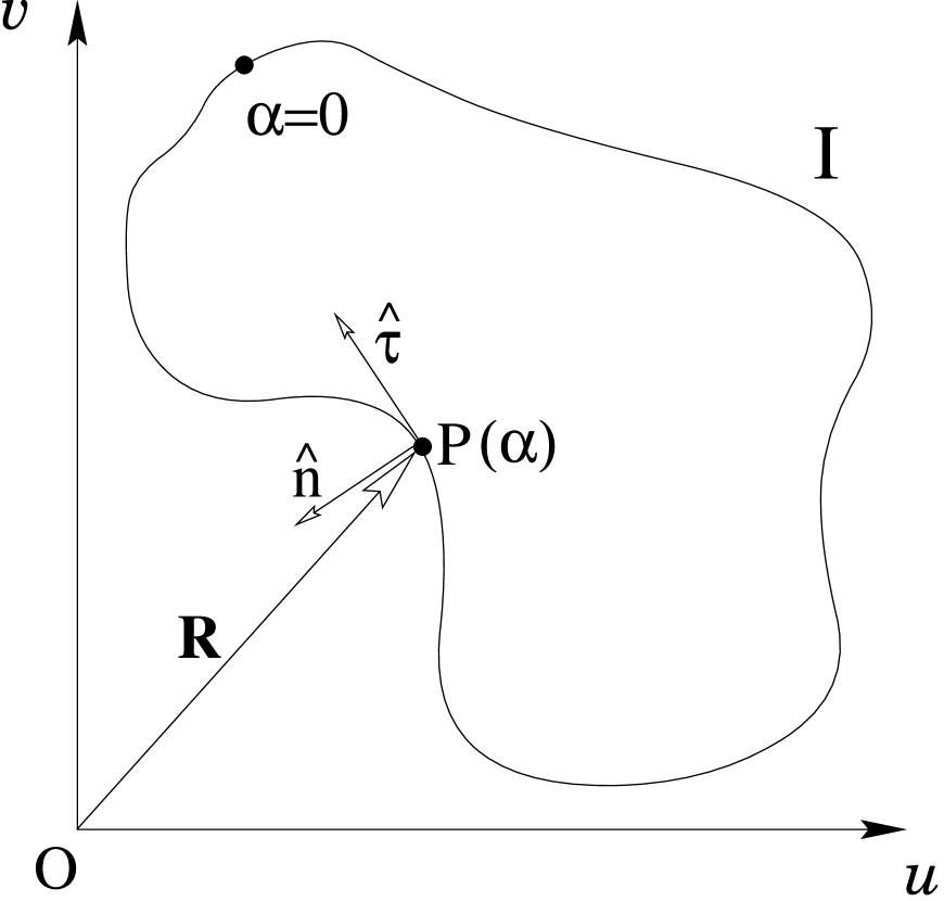
Figure 1: An interface $I$ in the $(u,v)$ space of the surface. A point $P$ of the interface has parameter $\alpha$ and is given by a vector ${\vec{R}}(P)$ (bold $R$ in figure). ${\hat{\tau}}$ and ${\hat{n}}$ are the tangent and normal vectors to $I$ at $P$.

A typical model-A interface, labelled $I$, is shown in Fig. 1, along with the vector ${\vec{R}}$ going from some arbitrary origin on the surface to a point $P(\alpha)$ on $I$, and the tangent ${\hat{\tau}}$ and normal ${\hat{n}}$ to the interface at $P$. Every point of an interface corresponds to a unique $\alpha$ which does not change in time, since the interface moves normal to itself.

The relationship between the differential elements of length $\mbox{d}s$ and $\mbox{d}\alpha$ is given by

$$\mbox{d}s=\sqrt{g}\;\mbox{d}\alpha.$$ (3)

where the metric is defined by

$$g(\alpha,t)\equiv\left|{\partial{{\vec{R}}}\over\partial\alpha}\right|^{2}.$$ (4)

Because $\mbox{d}\alpha$ is constant in time while $\mbox{d}s$ is not, $g$ changes in time. Its evolution equation must be determined, making use of the requirement that a point of coordinate $\alpha$ moves only perpendicularly to the interface. This can be done in the following way.

First note that ${\hat{\tau}}$ and ${\vec{\nu}}$ are defined as:

$${\hat{\tau}} \equiv {\partial{{\vec{R}}}\over\partial s}=(u^{\prime},v^{\prime})$$ (5)

$${\vec{\nu}} \equiv {\left({\partial{{\vec{R}}}\over\partial t}\right)_{\!\!\alpha}},$$ (6)

where a prime denotes differentiation relative to the arclength $s$. Taking the time derivative at constant $\alpha$ on both sides of Eq. (4), we have

$${\left({\partial{g}\over\partial t}\right)_{\!\!\alpha}} = 2{\partial{\vec{R}}\over\partial\alpha}\cdot{\left({\partial\over\partial t}{\left({\partial{\vec{R}}\over\partial\alpha}\right)}\right)_{\!\!\alpha}}$$ (7)

$$= -2{\partial^{2}{{\vec{R}}}\over\partial\alpha^{2}}\cdot{\vec{\nu}}.$$

Now since

$$\alpha^{\prime} \equiv {\partial{\alpha}\over\partial s}={{1}\over{\sqrt{g}}}$$ (8)

$$\alpha^{\prime}{}^{\prime} \equiv {\partial^{2}{\alpha}\over\partial s^{2}}={-1\over 2g^{2}}{\partial{g}\over\partial\alpha},$$ (9)

the Laplacian in arclength $s$ is

$${\partial^{2}{}\over\partial s^{2}}={1\over g}{\partial^{2}{}\over\partial\alpha^{2}}+\alpha^{\prime}{}^{\prime}{\partial{}\over\partial\alpha}$$ (10)

so that from the definition of the (three-dimensional) interface curvature vector ${\vec{K}}\equiv{\partial^{2}{{\vec{R}}}\over\partial s^{2}}$,

$${\partial^{2}{{\vec{R}}}\over\partial\alpha^{2}}=g\left({\vec{K}}-{\hat{\tau}}\alpha^{\prime}{}^{\prime}\sqrt{g}\right).$$ (11)

Substituting Eq. (11) in Eq. (7), using the orthogonality between ${\vec{\nu}}$ and ${\hat{\tau}}$ and rewriting Eq. (7) in terms of $\sqrt{g}$ rather than $g$ one obtains

$${\left({\partial{\sqrt{g}}\over\partial t}\right)_{\!\!\alpha}}=-\sqrt{g}{\vec{K}}\cdot{\vec{\nu}},$$ (12)

which further reduces to

$${\left({\partial{\sqrt{g}}\over\partial t}\right)_{\!\!\alpha}}=-\sqrt{g}{\vec{K}}_{g}\cdot{\vec{\nu}},$$ (13)

when one notes that ${\vec{\nu}}$ is parallel to ${\hat{n}}$ and lies within the surface, whereas ${\vec{K}}$ has a component parallel to ${\vec{\nu}}$ and one normal to the surface. I.e., if the normal to the surface is denoted by $\hat{N}$, then ${\vec{K}}=|{\vec{K}}_{g}|{\hat{n}}+|{\vec{K}}_{n}|\hat{N}$, with ${\vec{K}}_{n}$ the three-dimensional curvature of a geodesic tangent to $I$ at $P$. Equation (2) and the evolution equation for $g$, Eq. (13), are two of the three interface equations that are used in our interface description.

Now we proceed with a similar but lengthier derivation for $(\partial K_{g}/\partial t)_{\alpha}$. The dot product of ${\hat{n}}$ with Eq. (11) yields

$${{\hat{n}}\over g}\cdot{\partial^{2}{{\vec{R}}}\over\partial\alpha^{2}}=|{\vec{K}}_{g}|.$$ (14)

Applying the time derivative and using the chain rule,

$${\left({\partial{|{\vec{K}}_{g}|}\over\partial t}\right)_{\!\!\alpha}}={{\hat{n}}\over g}\cdot{{\partial^{2}\over\partial\alpha^{2}}{{\left({\partial{{\vec{R}}}\over\partial t}\right)_{\!\!\alpha}}}}-{{\hat{n}}\over g^{2}}\cdot{\partial^{2}{{\vec{R}}}\over\partial\alpha^{2}}{\left({\partial{g}\over\partial t}\right)_{\!\!\alpha}}+{1\over g}{\left({\partial{{\hat{n}}}\over\partial t}\right)_{\!\!\alpha}}\cdot{\partial^{2}{{\vec{R}}}\over\partial\alpha^{2}}.$$ (15)

The second term is simplified via Eq. (14) and Eq. (13). The third one is simplified by using Eq. (11) and noting that ${\hat{n}}$ can only change in direction, hence ${\left({\partial{{\hat{n}}}\over\partial t}\right)_{\!\!\alpha}}$ is oriented along ${\hat{\tau}}$. With those simplifications one gets

$${\left({\partial{|{\vec{K}}_{g}|}\over\partial t}\right)_{\!\!\alpha}}={{\hat{n}}\over g}\cdot{\partial^{2}{{\vec{\nu}}}\over\partial\alpha^{2}}+2|{\vec{K}}_{g}|{\vec{K}}_{g}\cdot{\vec{\nu}}-{\sqrt{g}}\alpha^{\prime}{}^{\prime}{\hat{\tau}}\cdot{\left({\partial{{\hat{n}}}\over\partial t}\right)_{\!\!\alpha}}$$ (16)

The second derivative of ${\vec{\nu}}$ is

$${\partial^{2}{{\vec{\nu}}}\over\partial\alpha^{2}}\equiv{{\partial^{2}\over\partial\alpha^{2}}{(\nu{\hat{n}})}}={\partial^{2}{{\hat{n}}}\over\partial\alpha^{2}}\nu+2{\partial{{\hat{n}}}\over\partial\alpha}{\partial{\nu}\over\partial\alpha}+{\hat{n}}{\partial^{2}{\nu}\over\partial\alpha^{2}}.$$ (17)

The first term is simplified by writing the second derivative of ${\hat{n}}$ in terms of arclength via Eq. (3), applying the chain rule and using the two Frenet equations for curves in Riemannian spaces[13]

$${\partial{{\hat{\tau}}}\over\partial s} = |{\vec{K}}_{g}|{\hat{n}}={\vec{K}}_{g}$$ (18)

$${\partial{{\hat{n}}}\over\partial s} = -|{\vec{K}}_{g}|{\hat{\tau}}.$$ (19)

This yields

$${\partial^{2}{{\hat{n}}}\over\partial\alpha^{2}}=-\sqrt{g}{\hat{\tau}}{{\partial\over\partial s}{(|{\vec{K}}_{g}|\sqrt{g})}}-g|{\vec{K}}_{g}|{\vec{K}}.$$ (20)

The second term of Eq. (17) vanishes when dot-multiplied with ${\hat{n}}$ given the second Frenet equation. After substitution of Eq. (17) and (20) in (16), we have

$${\left({\partial{|{\vec{K}}_{g}|}\over\partial t}\right)_{\!\!\alpha}}={1\over g}{\partial^{2}{\nu}\over\partial\alpha^{2}}+|{\vec{K}}_{g}|{\vec{K}}_{g}\cdot{\vec{\nu}}-\sqrt{g}\alpha^{\prime}{}^{\prime}{\hat{\tau}}\cdot{\left({\partial{{\hat{n}}}\over\partial t}\right)_{\!\!\alpha}}.$$ (21)

Finally we show that $\sqrt{g}{\hat{\tau}}\cdot{\left({\partial{{\hat{n}}}\over\partial t}\right)_{\!\!\alpha}}$ in the last term of Eq. (21) satisfies

$$\sqrt{g}{\hat{\tau}}\cdot{\left({\partial{{\hat{n}}}\over\partial t}\right)_{\!\!\alpha}} = -\sqrt{g}{\partial{\nu}\over\partial s}$$ (22)

$$= -{\partial{\nu}\over\partial\alpha}$$ (23)

It is easiest to show this by first deriving ${\partial{\nu}\over\partial s}$. The norm of the velocity is

$$\nu={\hat{n}}\cdot{\left({\partial{{\vec{R}}}\over\partial t}\right)_{\!\!\alpha}}$$

Taking the arclength derivative and using the chain rule,

$${\partial{\nu}\over\partial s} = {{\hat{n}}\over\sqrt{g}}\cdot{{\partial\over\partial\alpha}{{\left({\partial{{\vec{R}}}\over\partial t}\right)_{\!\!\alpha}}}}+{\left({\partial{{\vec{R}}}\over\partial t}\right)_{\!\!\alpha}}\cdot{\partial{{\hat{n}}}\over\partial s}$$ (24)

$$= {{\hat{n}}\over\sqrt{g}}\cdot{\left({\partial\over\partial t}{\left({\partial{{\vec{R}}}\over\partial\alpha}\right)}\right)_{\!\!\alpha}}$$ (25)

since ${\vec{\nu}}$ is orthogonal to ${\partial{{\hat{n}}}\over\partial s}$. Using ${\hat{\tau}}={\partial{{\vec{R}}}\over\partial s}$ and the chain rule again yields

$${\partial{\nu}\over\partial s} = {\hat{n}}\cdot{\left({\partial{{\hat{\tau}}}\over\partial t}\right)_{\!\!\alpha}}$$ (26)

$$= -{\hat{\tau}}\cdot{\left({\partial{{\hat{n}}}\over\partial t}\right)_{\!\!\alpha}}$$ (27)

where the second equality is obtained by using $\mbox{d}({\hat{\tau}}\cdot{\hat{n}})/\mbox{d}t=0$, completing the demonstration.

Thus, substituting Eq. (23) into Eq. (21) and using Eq. (10), we get the last of the three curvature equations:

$${\left({\partial{|{\vec{K}}_{g}|}\over\partial t}\right)_{\!\!\alpha}}={\partial^{2}{\nu}\over\partial s^{2}}+|{\vec{K}}_{g}|{\vec{K}}_{g}\cdot{\vec{\nu}}$$ (28)

The three equations, Eq. (2), Eq. (13) and Eq. (28), are a coupled set of curvature equations describing the evolution of interfaces in the Non Euclidean Model A. Note that in these equations, if two-dimensional vectors are used, the scalar product must be properly defined via the surface’s covariant metric tensor $g_{ij}\equiv{\partial{\vec{X}}\over\partial u^{i}}\cdot{\partial{\vec{X}}\over\partial u^{j}}$, i.e. $\tilde{a}\cdot\tilde{b}\equiv a_{i}g^{ij}b_{j}=a^{i}g_{ij}b^{j}$, where an implicit sum over alternate repeated indices is assumed. Equation (28) and Eq. (13) are purely geometric but only valid in the normal gauge and when ${\vec{\nu}}$ is parallel to ${\hat{n}}$.

The first term on the right hand side of Eq. (28) is diffusive and causes all modes of $K_{g}$ to dissipate, except the zeroth mode ($K_{g}=0$) which is not affected by it. The diffusive term thus seeks to shrink interfaces either into straight lines (on a curved surface, geodesics) which have zero $K_{g}$, or perfect (i.e. geodesic) circles which have constant $K_{g}$. On the other hand, due to the Non-Euclidean Interface Velocity equation, the second term on the right hand side of Eq. (28) is cubic in $K_{g}$. It seeks to increase the curvature and dominates when the diffusive term is negligible, i.e. for straight lines and circular domains. Hence it causes circular domains to shrink in radius, as is indeed the case in Euclidean model A. If the circular domain is also a geodesic, so that $K_{g}=0$ everywhere along the interface, the domain will not change in shape. When the model-A dynamics proceeds from a quench of a system from a high temperature, such that the domains are initially very disordered, the diffusive term of Eq. (28) dominates, broadly speaking, during the early stages of interface motion, whereas the cubic term dominates only in interfaces which have become circular. However, this was verified in numerical simulations to be only approximately true.

Another interesting aspect of the geometric equations is that substitution of Eq. (2) into Eq. (13) shows how ${\left({\partial{\sqrt{g}}\over\partial t}\right)_{\!\!\alpha}}$ is always negative. Therefore the distance between close-by interface points always decreases in time, and by extension also the total length of an interface, which is given by $L=\int\!\sqrt{g}\mbox{d}\alpha$:

$${\left({\partial{L}\over\partial t}\right)_{\!\!\alpha}}=-M\xi^{2}\int\!\!|{\vec{K}}_{g}|^{2}\;\mbox{d}s.$$ (29)

Without these results it is difficult to ascertain whether Eq. (2) is consistent with the physical nature of the bulk equation for model A kinetics, where the quantity of order-parameter gradients (equivalent to the total length of interface in the system) should monotonically decrease in time.

The apparent simplicity of the Non-Euclidean Interface Velocity equation can be misleading. The geodesic curvature of a line on a curved manifold depends both on the position of that line and its orientation on the surface. Therefore, $K_{g}$ introduces into the dynamics a new, position- and orientation-dependent length scale. This strongly suggests that Non Euclidean Model A dynamics cannot be self-similar as it is in flat systems, and therefore that dynamical scaling will not be observed on curved surfaces, except perhaps on self-affine surfaces, such as found over a certain range of length scales in lipid bilayer membranes. Different surfaces should show different phase-ordering kinetics. This is further evidenced in Eq. (29) where $L$ — proportional to the reference length scale of the dynamics, if it is present[18] — depends on $\int|K_{g}|^{2}\mbox{d}s$.

Nonetheless, a study of Non Euclidean Model A on the torus manifold, reported in [7], revealed no clear signature of the non-Euclidean nature of the surface when investigated through the evolution of the interface density (quantity of interface per unit area) and the $\lambda$-structure factor [19] of the order parameter. The latter is a two-dimensional order parameter structure factor which depends only on the intrinsic geometry of the surface and the order-parameter configurations. This absence of signature may be due not only to the coarse-grained nature of the $\lambda$-structure factor, but also to finite size effects, since domains feel the geometry only when their size becomes comparable to the torus size. This suggests that surfaces with geometrical features closer to those of model-A domains at early times should be investigated. Indeed, as we show in section 6, interfaces can get caught around certain surface bumps, causing a drastic slowing down and even immobilization of the model-A dynamics. Before investigating this, we outline the numerical methods used in the simulations.

3 Numerical method

It is customary to simulate equation for model A kinetics by discretizing them and evolving the order-parameter configurations via an Euler integration scheme. The main limitation of such discretization schemes is that the time step for evolving the system is limited by the smallest space mesh in the system. On curved surfaces, this can be — and most often is — a severe impediment, as the surface mesh can rarely be optimized so as to be homogeneous. Doing this involves computational challenges in its own right. Slightly more sophisticated methods such as spectral, predictor-corrector and implicit schemes are possible but the stiffness of the model-A kinetic equation still induces strong dependencies on spatial mesh which make them unappealing.

We have found that using Eq. (2) as the basis for an interface description has many advantages over a bulk description as given by a model A equation. Namely, the quantity of information to manipulate at every time step is an order of magnitude smaller at the beginning of the simulation than with a bulk description, and rapidly decreases in time, while for the bulk description it remains constant in time, even if the order-parameter configuration has become completely homogeneous. Secondly, the surface can be discretized independently from the interfaces so that numerical instabilities associated with the surface mesh disappear. Thirdly, the interfaces being one-dimensional, the integration algorithms remain fairly simple and more sophisticated algorithms are much easier to implement. Finally, certain quantities of interest, which we introduce below, are far easier and faster to compute from the interfaces than from the bulk configurations.

One inevitable drawback of an interface description is that it cannot describe how interfaces form from the small order-parameter fluctuations present just after the quench. Therefore, the initial interface configurations must be obtained independently. The easiest way to do this is of course to use the bulk description to evolve the order parameter for only the relatively short time necessary for interfaces to become established, and then extract the interfaces from the resulting configurations. Even for short integration times, this suffers from the drawbacks mentioned above. We give one alternative, in appendix C of [16], devoid of any bulk steps and dependent only on the statistical properties of interfaces.

For this reason, initial interface configurations are always obtained by integrating the bulk equation (1) from $t=0^{+}$ to $t=17$, when the domains have fully formed and interfaces can be extracted. For integration of bulk equations on curved surfaces, [20] has proved invaluable. Once the bulk configurations are obtained, the interface extraction is done with a program which we refer to as geninterf. A full-length run, done by a program we refer to as IFinteg, then takes the interface configurations from $t=17$ to $t=10000$. Such long runs were necessary in Non Euclidean Model A due to the slowing down of the dynamics at later times. A typical initial interface configuration is shown in Fig. 2, as would be seen in flat systems and in surfaces whose geometric features are much larger than the size of the initial interface convolutions.

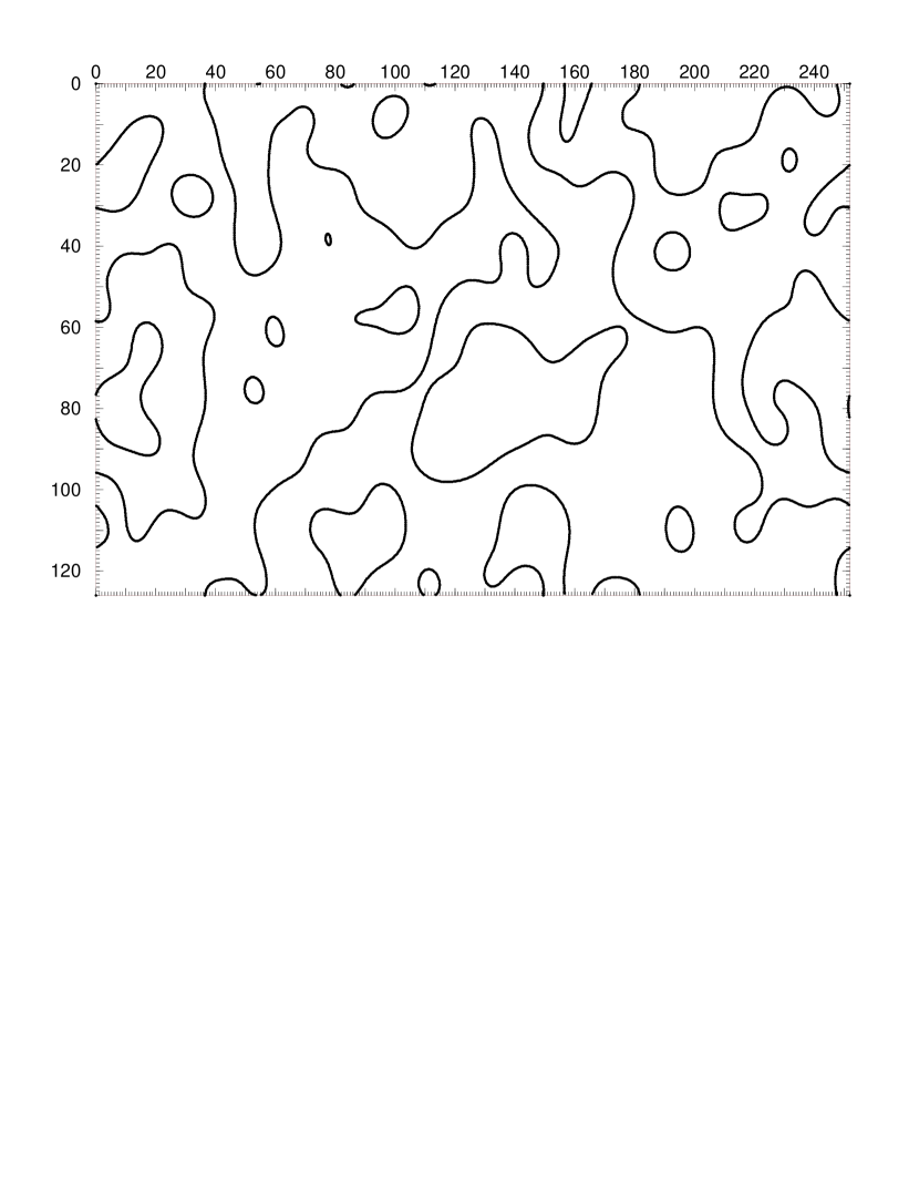
Figure 2: A typical early-time configuration of interfaces in a flat system.

An interface represented by its ordered set of coordinate points ${\tilde{R}}(\alpha)$ is evolved in the tangent space $(u^{1},u^{2})(\equiv(u,v))$ of the surface via the Non-Euclidean Interface Velocity equation by writing the latter in the form

$${\left({\partial{u^{i}}\over\partial t}\right)_{\!\!\alpha}}=M\xi^{2}K_{g}n^{i}$$ (30)

where $n^{i}$ is the $i^{th}$ component of the interface normal ${\tilde{n}}$, and $K_{g}$ is given, in compact notation, by

$$K_{g}=\epsilon_{ij}u^{i}{}^{\prime}(u^{j}{}^{\prime}{}^{\prime}+\Gamma^{j}_{kl}u^{k}{}^{\prime}u^{l}{}^{\prime})$$ (31)

where again implicit summation over repeated indices $\{i,j=1,2\}$ is assumed. The prime denotes differentiation with respect to arclength. Arclength is always the physical length of the curve as measured in the Euclidean embedding space of the surface. $\epsilon_{ij}$ is $(j-i)\sqrt{g_{m}}$, with ${g_{m}}=g_{11}g_{22}-g_{12}g_{12}$ the determinant of the metric of the manifold rather than that of the interface, which is $\sqrt{g}$. Equation (31) defines $K_{g}$ as a signed scalar, therefore ${\tilde{n}}$ is defined as ${\tilde{\tau}}$ rotated by $\pi/2$ counterclockwise and requiring ${\tilde{n}}\cdot{\tilde{\tau}}=0$, leading to

$${\hat{n}}={1\over\sqrt{g_{m}}}(-v^{\prime}g_{22}-u^{\prime}g_{12},u^{\prime}g_{11}+v^{\prime}g_{12}).$$ (32)

The numerical integration of Eq. (30) for the $j^{\mbox{\scriptsize th}}$ interface point is done by first computing $\sqrt{g_{m}}$ and $\sqrt{g}$ at the point, using these to obtain $K_{g}$ from Eq. (31) and ${\tilde{n}}$ from Eq. (32), and then by moving the point via the time map

$$u^{i}(j,t+\Delta t)=u^{i}(j,t)+\Delta tM\xi^{2}K_{g}(j,t)n^{i}(j,t);i=1,2$$ (33)

This Euler scheme becomes unstable if the discrete time step $\Delta t$ is too large. With the $\alpha$ parameter equal to the index of a point along the interface, $\sqrt{g}$ is the physical distance between points. Therefore, each interface is evolved with its own time step $\Delta t=0.4{\Delta t_{\mbox{\scriptsize{max}}}}$, with

$${\Delta t_{\mbox{\scriptsize{max}}}}\equiv{\scriptstyle\frac{1}{2}}(\sqrt{g}_{\mbox{\scriptsize{min}}})^{2}$$ (34)

and $\sqrt{g}_{\mbox{\scriptsize{min}}}$ is the smallest distance between two neighboring points of the discrete interface. As the integration proceeds, $\sqrt{g}_{\mbox{\scriptsize{min}}}$ decreases, which forces a decrease of $\Delta t$. For this reason, the interface is remeshed with all points separated by a distance of 1 unit whenever $\sqrt{g}_{\mbox{\scriptsize{min}}}<0.5$. The remeshing algorithm can be made very efficient, one remeshing requiring barely more than a few integration steps. In flat systems, the interface description is roughly 5 times faster than the bulk description. On curved surfaces, the gain increases dramatically: it was 50 or 100-fold in the simulations reported here, and will be much higher for more complex surfaces. Simulations using only the bulk description require, for a batch of 40 runs on the type of surfaces used here, on the order of 60 to 80 days on an HP9000s735.

The integration algorithm was verified for correctness and accuracy through several independent checks. Notably, the Non-Euclidean Interface Velocity equation can be solved exactly for a circular domain in a flat system. The simulation of such a domain yielded a curve indistinguishable from the theoretical prediction. Statistical runs starting from random initial order-parameter configurations were done with both bulk and interface descriptions and compared by measuring the amount of interface per unit area and comparing interface configurations and curvatures. Differences smaller than the interface width were found for the configurations, while the dynamical growth exponent of domains in flat systems was found to be $0.48\pm 0.01$ with the interface description, closer to the theoretical prediction of 1/2 than the bulk numerical integration result of $0.45\pm 0.02$. The interface description is hence favored if only in accuracy.

Simulations were also done on the torus manifold with both the bulk and interface descriptions and found to be once more identical apart from the similar difference in the dynamical exponents. In general, the interface description provides more accurate results than the bulk description, as seen by repeating the simulation of a band domain on a torus manifold[7, 16] for different surface mesh coarseness. The interface velocity from the bulk description converges towards the Non-Euclidean Interface Velocity theoretical prediction as the surface mesh is refined, while that from the interface description falls exactly on the theoretical prediction for all surface meshes used. This is shown in Fig. 3 where $\nu(t)$ is the interface velocity, and $\theta_{I}$ the Interface position on the torus (the torus manifold with its coordinate system and manifold are shown below in Fig. 5).

Figure 3: Interface velocity of stripe domain as a function of $\theta_{I}$ on the torus; $R=40,r_{0}=20$. Numerical simulation with $\Delta\theta=0.5$ (circles) and 1 (squares), and analytical prediction (line) are shown. At $t=0$ both top and bottom interfaces are near the outside equator of the torus.

Finally, as a further accuracy check, a circular domain on a surface consisting of one circular bump was simulated as the interface equations can be solved analytically. With the surface defined by

$${\vec{X}}=\left[u,v,Ae^{-(u^{2}+v^{2})/2\sigma^{2}}\right],$$ (35)

with $A$ the amplitude of the bump and $\sigma$ its half-width, the relationship between $K_{g}$ and the radius $R$ of the domain is

$$K_{g}R={1\over\sqrt{1+\left({A\over\sigma}\right)^{2}\left({R\over\sigma}\right)^{2}e^{R^{2}/\sigma^{2}}}}$$ (36)

The comparison of the theoretical prediction and numerical simulation is shown in Fig. 4 where the product $K_{g}R$ is plotted vs $R$. Two different surface meshes were used, showing what kind of surface coarseness is sufficient for accurate results: the longest surface tether should be around 0.7 units long for best results, though 1.3 units gave satisfactory results as well, as seen in the figure.

Figure 4: $K_{g}R$ of a circular domain as a function of its radius $R$, as given by numerical integration on 2 different grid sizes; also shown is analytical prediction eq. (36). Error bars too small to be seen.

4 Effects of surface curvature on domain growth

A naive interpretation of the Non-Euclidean Interface Velocity equation may suggest that Non Euclidean Model A dynamics should always be slower than Euclidean dynamics: $|{\vec{K}}_{g}|$ is always less than or equal to the total interface curvature $|{\vec{K}}|$. However diffusion occurs faster (slower) in regions of negative (positive) surface Gaussian curvature $K_{G}$[12], because there is more (less) area available for a given interface length in a region of negative (positive) $K_{G}$[21]. This suggests that interfaces arising from the Non Euclidean Model A equation should disappear more slowly where $K_{G}>0$, but faster where $K_{G}<0$. Yet, simulations of the Non Euclidean Model A on the torus manifold, starting from random initial order-parameter configurations, showed no dependence whatsoever on Gaussian curvature[7]. This may have been due to the use of the $\lambda$-structure factor [19] as the measure of the two-dimensional Order Parameter Structure Factor or to the combination of the topology of the torus with the percolating domains.

To settle the matter, one ovoid interface was therefore simulated in the $K_{G}>0$ region of the torus manifold, another in the $K_{G}<0$ region and again in a flat system ($K_{G}=0$). The torus manifold is convenient for many reasons discussed in [7], most importantly that two well-separated regions of oppositely signed Gaussian curvature can be defined on the torus. A drawing of part of a torus surface with coordinates and parameters is shown in Fig. 5.

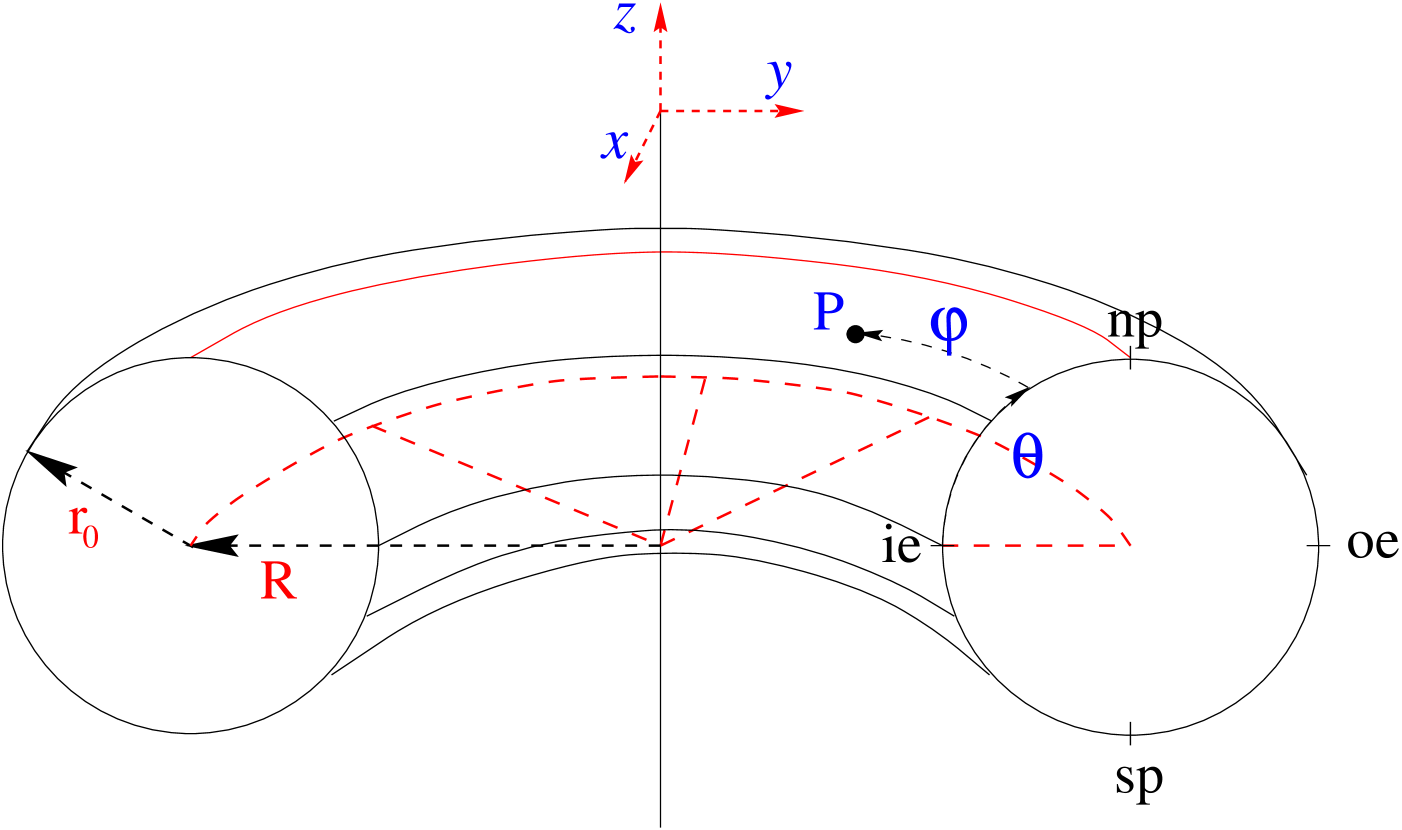
Figure 5: Torus manifold of long radius $R$ and small radius $r_{0}$. Point $P$ on manifold has coordinates $(u^{1},u^{2})\equiv(\theta,\varphi)$. $\theta=0$ and 1 are at inner equator (labelled “ie”), $\theta=\pi r_{0}$ is at the outer equator (labelled “oe”).

The small radius of the torus is denoted $r_{0}$ and the large one $R$. The initial radius of the ovoid is such that it is completely included in the appropriate region of the torus, i.e. $\pi r_{0}/2$ as measured in $(\theta,\varphi)$ space (see Fig. 5).

Figure 6 shows a log-log plot of $-\mbox{d}L/\mbox{d}t$ as a function of $1/L$, where $L(t)$ is the time-dependent length of the ovoid interface in the system.

Figure 6: Log-log plot of $-\mbox{d}L/\mbox{d}t$ vs $1/L$. Straight line is for simulation of flat system. The scatter for nonzero $K_{G}$ is due to numerical discretization of the surface.

A straight line is obtained in the flat system, as expected for Euclidean model A. However, differences as large as a factor of two can be seen at early times with the curved regions, when the domains are large (roughly 20% of system area). The difference remains substantial until the domains are very small. This suggests that the absence of visible non-Euclidean effects reported in [7] could be a characteristic of the $\lambda$-structure factor. Note that the oscillations for the $K_{G}\neq 0$ curves are due to the numerical discretization of the torus manifold.

The above simulation result can be understood analytically with the help of Eq. (13) by considering surfaces of constant Gaussian curvature (i.e., a sphere, a flat plane, and a hyperbolic plane). In this case, a circular domain remains circular, as indicated by Eq. (28), i.e. the geodesic curvature is constant everywhere along the interface at any given time (but changes in time). Integrating both sides of Eq. (13) along the interface then yields $-\mbox{d}L/\mbox{d}t\sim LK_{g}^{2}$, where $K_{g}$ is a function of time (note also Eq. (29)). It is useful to express $K_{g}$ in terms of $K_{G}$. In a flat system $K_{g}^{2}=4\pi^{2}/L^{2}$ when the domain boundary has length $L$. For small $K_{G}\neq 0$, dimensional analysis indicates the first order correction to $K_{g}^{2}$ when in a curved surface should be of the form $\gamma K_{G}$, with $\gamma$ a dimensionless geometrical factor of the order of 1. Moreover, when $K_{G}$ is increased from 0 (i.e. the surface is a sphere of decreasing radius) while keeping $L$ constant, the geodesic curvature monotonically decreases, until it eventually becomes 0 when $K_{G}=(2\pi/L)^{2}$. On the other hand, when $K_{G}$ is increased negatively from 0 (i.e. the surface is a hyperbolic plane), the area available to the circular domain increases, such that in order to keep $L$ constant, the radius of the domain must be decreased, increasing the geodesic curvature. This leads to the first order approximation for the time change of the circular domain’s interface length,

$$-{\mbox{d}L\over\mbox{d}t}\sim{4\pi^{2}\over L}\left(1-{\gamma L^{2}K_{G}\over 4\pi^{2}}\right),$$ (37)

with $\gamma>0$, providing a qualitative explanation the difference in growth laws for the ovoid domains in regions of different Gaussian curvature.

Given the physical origin of the influence of the surface Gauss curvature $K_{G}$ on domain growth in the Non Euclidean Model A, much the same can be expected in non-Euclidean model B as well as in other systems where diffusion and interfaces are present on curved surfaces. This slowing down for positive $K_{G}$ was not observed in numerical simulations of pure model B on the static sphere[9], because of the short run times used. However, similar (though not identical) Gauss curvature effects were seen in simulations of crystal growth on toroidal geometries[2]. In the context of phase-ordering kinetics and phase-separation in lipid bilayers, where diffusion is known to play a very important role biologically, this dependence on $K_{G}$ could be of use in controlling the rate of such processes as protein diffusion via membrane shape change, or inducing enzyme-protein interaction in limited parts of a cell.

5 Simulations on sinusoid surfaces

When the initial order-parameter configuration is one of complete disorder, the non-linear regime of Euclidean model A is characterized by the relatively slow motion of sharp, convoluted interfaces delimiting domains of $\phi=\pm 1$ phases. There are two characteristics of Euclidean-model-A dynamics which are particularly important here. First is the self-similarity of the dynamics, leading to dynamical scaling: system configurations at a time $t_{1}$ look statistically identical to configurations at an earlier time $t_{0}$, if they are rescaled lengthwise by an appropriate factor. Hence all dynamical lengths in the system have the same time dependence, so that they can all be expressed in terms of one arbitrarily chosen reference length scale $L(t)$. The numerical value of $L$ is not as important as its time dependence, which is the second characteristic of relevance: $L(t)\sim t^{1/2}$.

It is common to refer to $L$ as a dominant or typical length scale in the dynamics, but the order parameter structure factor for Euclidean-model-A systems shows a peak at zero wavenumber, indicating model-A dynamics does not have a dominant length scale, only a unique time dependence for all dynamical lengths. We have shown for the first time[16, 18], by considering the curvature correlations along the interface, that Euclidean-model-A systems exhibit a dominant undulation mode not present in the order-parameter structure factor. If one is to talk of a dominant dynamical length in model A, it is the wavelength of this undulation, not the width of the order parameter structure factor. This suggests it has a different nature from that of Euclidean model B, where the dynamical length is visible in the order parameter structure factor. Notably, the absence of the dominant dynamical length in model A’s order parameter structure factor may be due to the absence of any phase information in it.

Now consider a surface consisting of a large array of bumps:

$${\vec{X}}=\left[x,y,A\sin\left({2\pi x\over\lambda}\right)\sin\left({2\pi y\over\lambda}\right)\right].$$ (38)

Experimentally, fluid as well as crystalline lipid bilayers are known to adopt a similar shape (called “egg carton”) under certain conditions[22]. Also, more complex surfaces such as self-affine surfaces common to fluctuating lipid bilayer membranes share many of the qualitative features of sinusoid surfaces.

Simulations of Non Euclidean Model A on sinusoid surfaces, starting with random initial order-parameter configurations, were done for several values of $A$ and $\lambda$, but here we focus on the $\lambda=20,A/\lambda=0.2$ surface, with system sizes of $100\times 100$ to $300\times 300$.

The normalized geodesic curvature autocorrelation function is defined by

$${G_{\!\mbox{\tiny$K_{g}$}}(s,t)}={\langle K_{g}(s_{0},t)K_{g}(s_{0}+s,t)\rangle\over\langle K_{g}(s_{0},t)^{2}\rangle},$$ (39)

where $\langle\ldots\rangle$ denotes an ensemble average with an average over all interface points $s_{0}$. It is plotted in Fig. 7,

Figure 7: ${G_{\!\mbox{\tiny$K_{g}$}}(s,t)}$ at various times from $t=35$ (long dashed) to $t=400$ (short dashed), vs $s/L(t)$. Sinusoid surface used is eq. (38) with $A=4,\lambda=20$. Inset: Variance of Gaussian part of ${G_{\!\mbox{\tiny$K_{g}$}}(s,t)}$ vs time (times between 17 and 700).

where the horizontal axis has been rescaled with $L(t)$, defined here as first zero of the geodesic curvature autocorrelation function, and the error bars (not shown for clarity[23]) are much smaller than the vertical offsets of the curves. In flat systems, as explained in [16, 18], all such geodesic curvature autocorrelation functions fall on top of one another, due to dynamical scaling. Figure 7 thus shows that for the non-Euclidean case, dynamical scaling breaks down, as expected from our discussion of Eq. (2) but contrary to runs on the torus manifold. The other important feature is that as time increases, the dominant interface undulation mode monotonically decreases in intensity, signifying the system’s degree of order decreases as the interfaces explore ever larger length scales. This is sensible given that when the dominant length is much smaller than the geometrical features of the surface, the interface correlations decay fast enough to become negligible. As the undulation wavelength increases, the correlations become negligible at increasing distances, introducing geometrical variations in the interface shape, thus increasing the degree of disorder in the system.

These two features — breakdown of dynamical scaling and existence of a dominant dynamical length — further confirm that the presence of a dominant dynamical length does not guaranty dynamical scaling.

Figure 7 also indicates that the first zero of the geodesic curvature autocorrelation function can no longer be used as a reference dynamical length. Two well-defined dynamical lengths valid for interfaces on curved surfaces are the width $\sigma$ of the Gaussian part of the geodesic curvature autocorrelation function, and the inverse interface density. Though ${G_{\!\mbox{\tiny$K_{g}$}}(s,t)}$ is found to remain Gaussian on short length scales, the time dependence of its width is no longer a $t^{1/2}$ power law, contrary to flat systems. For the sinusoid surface used here, it was found to be logarithmic. The logarithmic law is shown in the inset graph to Fig. 7, where linear regression gives $\sigma^{2}\simeq(63\pm 3)\log_{10}(t/t_{0})$, with $t_{0}=6\pm 2$. This logarithmic time dependence is not a universal feature, as sinusoid surfaces with smaller values of $A/\lambda$ showed power-law growth but slower than $t^{1/2}$. It seems likely that a sub-logarithmic growth law will be seen for larger $A/\lambda$, similarly to results reported in [24] on the related Random-Field Ising Model. The width $\sigma$ can be used as the reference length scale $L(t)$ to rescale the geodesic curvature autocorrelation function, as shown in Fig. 8. The inset shows the result for flat systems, exhibiting dynamical scaling, within error bars. The main graph shows the result for the sinusoid surface. There the curves superpose only on short length scales, while at long length scales they systematically become wider, with the drift being much larger than the error bars.

Figure 8: Main graph: Same as main graph of Fig. 7 but using $L(t)=\sigma(t)$ to rescale ${G_{\!\mbox{\tiny$K_{g}$}}(s,t)}$. Inset: Same as main graph but for flat systems.

While the width of the geodesic curvature autocorrelation function is a short-length-scale characteristic of the dynamics, the interface density is more sensitive to large-scale features. It is defined as $l(t)\equiv L(t)/A_{s},$ where $L(t)$ is the total length of interfaces at time $t$ and $A_{s}$ is the system area (constant in time). Measurements of $l(t)$ for the sinusoid surface were done and compared with those in flat systems of various sizes. This is shown in Fig. 9, where $-d(\ln l)/dt$ is plotted as a function of $1/l^{2}$.

Figure 9: Logarithmic plot of $\mbox{d}\ln(l)/\mbox{d}t$ as a function of $1/l^{2}$, for sinusoid surface $A=4$ and $\lambda=20$ (circles). Points for flat system are triangles and squares, lines are linear regressions. Error bars (not shown) are approximately same size as symbols.

This scale produces one unique curve for all flat systems, independent of system size or quantity of interface. Any straight line on this plot indicates a power law in time for $\ell(t)$. If the slope of the line is denoted $m$, the intercept $b$ and $\ell_{0}\equiv\ell(0)$, then straightforward integration yields

$$\ell(t)=\left(\ell_{0}^{2m}-2m10^{b}t\right)^{1\over 2m},$$ (40)

indicating $\ell\sim t^{1/2m}$ at late times. More negative $m$ thus corresponds to slower interface dynamics. The interface density has units of one over length, while the dominant length scale in Euclidean model A grows as $t^{1/2}$. Hence the scaling assumption valid for flat systems predicts $\ell\sim t^{-1/2}$, i.e. $m$ should be equal to -1 in flat systems. The linear regressions for the flat system curve (where bulk integration was used rather than the interface description) gives $m=-1.07\pm 0.01$, which means a power law of $-0.46\pm 0.01$ instead of -1/2.

At early times (small values of $1/\ell^{2}$), model-A dynamics on the sinusoid surface also follows the same power law. At later times however, one can distinguish a fairly long time regime, extending from $t\simeq 250$ to $t\simeq 1600$, almost a full decade of time, during which $m$ is more negative. The dynamics has therefore substantially slowed down. Linear regression in this time domain gives $m=-1.70\pm 0.04$, corresponding to a power law behavior for $\ell$ of $t^{-0.3}$. A batch of runs for a smaller system of size $100\times 100$ gave $m=-2.0\pm 0.1$, suggesting the statistical error on the slope could be as large as 20 to 30%.

A very interesting characteristic of this plot is the presence of a very late time regime, where the dynamics is extremely slow, with the slope $m=-8\pm 2$. This starts at $t\simeq 2000$, independent of system size and discretization. Real-time animation of moving interfaces in this regime shows that the geodesic curvature is zero almost everywhere, but not in sufficiently many places to completely halt the dynamics. The interfaces, which waver between the bumps, are very slowly hopping the bumps one by one.

6 Metastable states

Corrugated surfaces (such as given by Eq. (38)) allow for local minima to appear in the configuration space of interfaces and therefore to trap the latter in metastable states, because Eq. (29) implies that Non Euclidean Model A interfaces can only decrease their length. The simplest example of this would be an ovoid interface circumventing two bumps on the sinusoid surface, as pictured in Fig. 10.

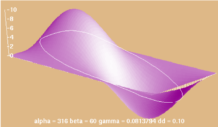
Figure 10: Three-dimensional view of the 2-bumps surface with the ovoid interface (white line). System size $40\times 20,A=10,\lambda=40$. Surface is shown as transparent to interface.

Consider the interface as it shrinks in length. It is forced to tilt itself, slowly moving on the outside towards the extremum of each bump. The total curvature at a point of the interface is the curvature as measured in three-dimensional embedding space. Recall that the total curvature vector ${\vec{K}}$ of a geodesic line on the surface is normal to the surface since $K_{g}=0$ for a geodesic. Therefore a necessary condition for the interface to become stationary is for a configuration to exist where ${\vec{K}}$, near both ends of the ovoid domain, is normal to the surface. A side view ($x-z$ projection) of the bumps with the interface is pictured in Fig. 11 and a top view ($x-y$ projection) in Fig. 12.

Figure 11: Side view of surface shown in Fig. 10 with projection of ovoid interface on $xz$ plane, at a later time when the interface is almost stationary, i.e. $\hat{n}$ and $\hat{K}$ are almost parallel.

Figure 12: Top projectional view for Fig. 11. Interface is thick line. $K$ is curvature vector, other symbols correspond to those in Fig. 11. Line $AB$ is “pivot” line for interface. Circles are contours for the surface.

This is not a sufficient condition however since all points along the interface must satisfy this criterion, but it does provide a minimal condition.

We now denote the vector going from $O$ to $P$ in Fig. 11 as ${\vec{R}}=[x,A\sin(kx)]$. The tangent to the surface in $P$ is therefore ${\hat{\tau}}=[1,Ak\cos(kx)]$, and the condition is ${\vec{R}}\cdot{\hat{\tau}}=0$, leading to the transcendental equation $2x=-A^{2}k\sin(2kx)$. With the substitution $x^{\prime}=2kx$ and $\gamma=Ak$ this is written

$$-{1\over\gamma^{2}}={\sin x^{\prime}\over x^{\prime}}.$$ (41)

This equation has a solution only when $\gamma$ is larger than a certain value, for when $\gamma\rightarrow 0$ the left hand side tends to $-\infty$ while the right hand side is bounded between 1 and roughly $-0.22$. The condition is therefore $-1/\gamma^{2}\gtrsim-0.22$, or

$${A\over\lambda}\gtrsim 0.34.$$ (42)

This was tested numerically for fixed $\lambda=40$. Simulations give a threshold of $0.42\pm 0.02$. This is an error of 20%, surprisingly good considering that the approximation uses a one-dimensional projection of the interface on the surface: it is not unusual for the presence of a second dimension to give a system more freedom, thereby softening constraints such as Eq. (42).

It is important to note that Eq. (42) is a necessary (minimal) condition for interfaces to get blocked around two bumps, and that blockage around a larger number of aligned bumps occurs at similar or larger values of $A/\lambda$. This can be seen by considering three aligned bumps instead of two. The middle bump constrains the interface to belong to the $xy$ plane in its vicinity, so that point $O$ of Fig. 11 still lies between bumps rather than, say, at the center of the middle bump. The condition Eq. (42) therefore still holds for any number of aligned bumps larger than or equal to two. This is sensible since what matters is $\lambda$, not the number of bumps.

However the situation is the reverse for bumps that are not aligned, which is more relevant with regards to the results of the Non Euclidean Model A simulations on sinusoid surfaces. Consider 4 bumps in a $2\times 2$ array, and an interface that circumnavigates the four bumps. A top projectional view is shown in Fig. 13.

Figure 13: Top projectional view for interface around four bumps. Same conventions are used as in Fig. 12. The pivot point is now $O^{\prime}$ rather than $O$.

Point $O$, one of the interface pivot points on segment $AB$, is still halfway between bumps, near the system boundary. The maximum-curvature director however no longer lies along $x$ but along the line $x=y$. Therefore, the pivot point normal to the interface at $P$ is at $O^{\prime}$ rather than $O$, decreasing the apparent wavelength by a factor of $\sqrt{2}$, so that smaller amplitudes (by the same factor) are sufficient to trap the interface. In this case the threshold decreases to 0.24, with simulations giving $0.270\pm 0.006$. The proximity to this threshold of $A/\lambda=0.2$ in the sinusoid simulations of the last section explains the existence of the very-late-stage, extremely-slow regime evidenced on Fig. 9.

The same kind of argument can be extended to, say, 6 bumps in a hexagonal configuration, bringing $O^{\prime}$ yet closer to $P$. For a large surface consisting of a great number of bumps, gradually increasing $A$ from zero should cause interfaces to become stationary first around very large conglomerates of bumps. However the larger the conglomerate must be, the rarer the occurrence. As $A$ is increased further, smaller conglomerates of bumps trap closed interfaces, until an $A$ is reached where the domains stop growing when the dominant interface undulation length becomes comparable to the surface $\lambda$, leading to long-range disorder.

The metastability thresholds can be generalized to more complex surfaces. For instance, lipid bilayer membranes are usually characterized by their bending rigidity $\kappa$. Such membranes form random self-affine surfaces whose average square width $W^{2}$ is given by[25]

$$W^{2}={L_{s}^{2}k_{B}T\over 4\pi^{3}\kappa}$$ (43)

where $L_{s}$ is the size of the membrane as projected on the $xy$ plane. The amplitude $A$ can be approximated by the width $W$ for a given size, while the wavelength $\lambda$ can be approximated by $L_{s}$. As a consequence of Eq. (42), phase ordering may not occur at all if $\kappa\lesssim k_{B}T/8$, as in this case Eq. (42) is satisfied on all length scales $L_{s}$. As $\kappa$ is decreased towards $k_{B}T/8$, the Non Euclidean Model A dynamics should gradually slow down. When $\kappa<k_{B}T/8$, domains might still form but freeze in their early disordered state.

For real systems the hopping condition on $\kappa$ is not likely to be as simple, since for such small values of $\kappa$ the surface tension $\sigma$ will usually be non negligible. The main difference is that the threshold involves $\kappa,\sigma$ and the length scale of interest, without introducing any new difficulty. This suggests that domains could order for some time, until their dominant interface undulation length becomes larger than a certain threshold value.

In flat systems, it was shown by Bray[26] that model A exhibits a zero-temperature strong-coupling fixed point. The existence of metastable interface configurations on corrugated surfaces implies that thermal noise changes the quality of the dynamics once the domain interface undulations are on the same scale as the surface corrugations, thereby eliminating the fixed point. Consequently, in the very-late-stage (i.e. extremely slow) regime observed on sinusoid surfaces, interfaces will move predominantly via thermally-activated hopping. Similar conclusions should be valid for model B. Effect of thermal noise needs to be carefully considered.

7 Total curvature correlations

There is a second form of curvature autocorrelation involving the total curvature ${\vec{K}}$ of the interface, i.e. the curvature of the interface measured in three-dimensional space rather than in the two-dimensional space of the manifold. In three dimensions, a curvature scalar can not be well defined. The vector of curvature is the only way to properly represent the curvature of the interface, so a dot product must be used in this case:

$${G_{\!\mbox{\tiny$\vec{K}$}}(s,t)}\equiv{\langle{\vec{K}}(0,t)\cdot{\vec{K}}(s,t)\rangle\over\langle{\vec{K}}(0,t)^{2}\rangle}.$$ (44)

Note that for flat systems, where the scalar product of two ${\vec{K}}_{g}$ is straightforward, both definitions of curvature autocorrelation, the total and the geodesic one, give the same function. It is only in curved surfaces that they differ in very important ways. In the curved case, when an interface is stationary, it is so only because $K_{g}$ is 0 everywhere and the interface is perfectly autocorrelated, from a two-dimensional point of view. This perfect autocorrelation stems from the fact that if two-dimensional observers within the manifold knew the position and orientation of the interface at one point of the interface, they would know the complete shape of the interface by solving the equations defining geodesics[13] with the appropriate initial values. The only disorder remaining in the system is that arising from the relative position of the domains and from the extrinsic geometry of the geodesic lines on the surface. This is not measurable via a geodesic curvature autocorrelation function.

On the other hand, the total curvature of a convoluted interface at early times, when the domains are much smaller than any geometric length scale of the surface, is equal to the geodesic curvature of the interface, in modulus. Under this condition the total and geodesic curvature autocorrelation function are nearly identical at early times (analytically they are rigorously equal). At late times, when an interface has become stationary, the total curvature at a point of the interface is the curvature of the surface along the direction of that interface. This total curvature autocorrelation function will therefore give information about the curvature autocorrelations of the surface along geodesic lines. This information is part of the extrinsic geometry of the surface and does not enter the geodesic curvature autocorrelation function. The two autocorrelation functions are therefore complementary for interface dynamics on curved surfaces.

When the interface correlations decay faster in space than the wavelength of the surface, ${G_{\!\mbox{\tiny$\vec{K}$}}(s,t)}$ is, as discussed earlier, qualitatively very close to ${G_{\!\mbox{\tiny$K_{g}$}}(s,t)}$. Both correlation functions are not exactly equal as the scalar product in ${G_{\!\mbox{\tiny$\vec{K}$}}(s,t)}$ produces a slightly stronger dip amplitude by about 20%, and the error bars are substantially smaller in ${G_{\!\mbox{\tiny$\vec{K}$}}(s,t)}$. Near the minimum they are as much as 3 times smaller. However, while the average $K_{g}$ decreases in time, the ${\vec{K}}$ eventually starts increasing until it reaches values compatible with the surface $\lambda$. Therefore, ${G_{\!\mbox{\tiny$\vec{K}$}}(s,t)}$ becomes very different from ${G_{\!\mbox{\tiny$K_{g}$}}(s,t)}$ at late times.

Figure 14 shows ${G_{\!\mbox{\tiny$\vec{K}$}}(s,t)}$ for the runs on the sinusoid surface, Eq. (38) with $A=4$ and $\lambda=20$, at times between 17 and 10000 (17, 35, 50, 100, 150… 400, 500, 700, 1000, 1200, 1450, 1750, 2100, 2500, 3000, 4000… 10000). The curves for $t=17$ and 10000 are labelled, with curves at intermediate times moving gradually and monotonically from the former to the latter.

Figure 14: ${G_{\!\mbox{\tiny$\vec{K}$}}(s,t)}$ for the sinusoid surface $A=4,\lambda=20$

For this surface, the wavelength of the bumps is not much larger than the initial dominant length scale of the interfaces in Euclidean systems, so that a cross-over regime is not seen. The correlations simply increase in time, as more and more interfaces coarsen while being pushed between the bumps and adopting the surface’s wavelength. At late times, the interfaces can be approximated by a random sequence of straight lines of length $\lambda/2$ and arcs of radius $\lambda/4$ and arclength $(\pi/4)\lambda/2$ . This explains the peak positions in ${G_{\!\mbox{\tiny$\vec{K}$}}(s,t)}$ being roughly at integer multiples of $(\pi/4)\lambda/2$. At early times, only two peaks can be seen, with a third peak starting to appear. The emergence of the peaks at larger distances seems to coincide with the Euclidean regime in Fig. 9. During the slow regime ($250\lesssim t\lesssim 1600$), no more peaks appear. Those that have formed grow slowly in amplitude and saturate. Figure 15 shows ${G_{\!\mbox{\tiny$\vec{K}$}}(s,t)}$ for a sinusoid surface consisting of two wavelengths rather than one:

$${\vec{X}}=[x,y,4\sin(2\pi k_{1}x)\sin(2\pi k_{1}y)+6.25\sin(2\pi k_{2}x)\sin(2\pi k_{2}y)]$$ (45)

where $\lambda_{1}=2\pi/k_{1}=40$ and $\lambda_{2}=2\pi/k_{2}=50$. Hence both have $A/\lambda\simeq 0.1$ and the undulations of this surface are of longer wavelength than the previous one.

Figure 15: ${G_{\!\mbox{\tiny$\vec{K}$}}(s,t)}$ for the bimodal sinusoid surface, eq. (45) with $\lambda_{1}=40$ and $\lambda_{2}=50$. Times are $t=17,24,35,60,100$ with the remaining times at same values as in Fig. 14.

In this case, the earliest curve looks exactly like $G_{\!\mbox{\tiny$K$}}^{2}(s,t)$ in flat systems and even has the dip positioned at roughly the same value, namely $s\simeq 10$. Already at $t=24$ the interfaces are being pulled into the valleys between the bumps. This is the crossover regime. The curvature correlations settle into their definitive value around $t=100$, close to $(\pi/4)\lambda/2$ with $\lambda$ around $40$. Much longer wavelengths would be necessary to distinctly show the three regimes: a scaling regime at early times during which the amplitude of the minimum would not change, then the cross-over during which the dominant length scale saturates to a dominant mode of the surface, and finally the late-time regime where the interfaces move more slowly and hop the bumps. Note that contrary to the $A=4,\lambda=20$ case, the very-late-stage regime of Fig. 9 never occurs because $A/\lambda$ is not large enough.

8 Summary and conclusions

In summary, the non-Euclidean model A was used as a starting point for the more complex, Random-Field Ising Model like[6, 27, 24] models used in some lipid membrane[28] and related surface problems. By deriving a set of geometric dynamical equations, using the non-Euclidean interface velocity equation ${\vec{\nu}}=M\xi^{2}{\vec{K}}_{g}$ and developing an interface description, numerical simulations of this difficult system could be carried out and the results analyzed and understood qualitatively. Moreover, the techniques should be applicable without major impediments to dynamical surfaces and model B on curved surfaces.

Whereas Random-Field Ising Model systems exhibit decelerated growth in the form of logarithmic growth laws of various kinds, here we have shown how model A on curved surfaces exhibit similar richness of dynamics without a bilinear coupling to the surface: (i) the time dependence of the amount of interface is strongly affected by the local Gaussian curvature of the surface, (ii) different dynamical lengths have different and even logarithmic time-dependencies leading to the breakdown of dynamical scaling without the disappearance of the dominant interface undulation mode, and (iii) metastable states exist above a threshold value of $A/\lambda$, leading to thermally activated hopping in the new very-late-stage regime. A more systematic study of the effect of $K_{G}$, a better quantitative understanding of the observed time dependencies of $L$, and experimental methods to obtain the dominant interface undulation mode, would be useful at this point.

References

- [1] R. Lipowsky and E. Sackmann, editors, Structure and Dynamics of Membranes: From Cells to Vesicles, volume 1A and 1B of Handbook of Biological Physics, Elsevier Science B. V., North-Holland, 1st edition, 1995.
- [2] P. Peczak, G. S. Grest, and D. Levine, Phys. Rev. E 48, 4470 (1993).
- [3] P. Petroff and G. Medeiros-Ribeiro, MRS Bulletin 21, 50 (1996).
- [4] C. Gebhardt, H. Gruler, and E. Sackmann, Z. Naturforsch. C 32, 581 (1977).
- [5] S. Leibler and D. Andelman, Journal de Physique 48, 2013 (1987); T. Taniguchi, K. Kawasaki, D. Andelman, and T. Kawakatsu, Journal de Physique II France 4, 1333 (1994).
- [6] E. K. Hobbie, Am. J. Phys. 64, 151 (1996).
- [7] O. Schönborn and R. C. Desai, Physica A 239, 412 (1997).
- [8] G. Gompper and M. Schick, Self-assembling amphiphilic systems, volume 14, Academic Press, London, 1994; S. A. Safran, Statistical thermodynamics of surfaces, interfaces, and membranes, volume 90 of Frontiers in Physics, Addison-Wesley Pub., 1994.
- [9] T. Taniguchi, Phys. Rev. Lett. 76, 4444 (1996).
- [10] P. B. S. Kumar and M. Rao, Phys. Rev. Lett. 80, 2489 (1998).
- [11] P. C. Hohenberg and B. I. Halperin, Rev. Mod. Phys. 49, 435 (1977).
- [12] See references [13] and [21] for further discussion of these notions. The total interface curvature is the curvature at a point of a line interface in three-dimensional space. Its geodesic curvature at that point is that component of the total curvature which lies within the surface. On the other hand, a surface has two orthogonal radii of curvature at every point on it, which can be of the same or opposite sign. The Gauss curvature is the product of these two curvatures. vanishes for a flat region of a surface, is positive in regions where the surface looks locally spherical, and is negative if the region is locally saddle-like.
- [13] D. Laugwitz, Differential and Riemannian Geometry, Academic Press, New York and London, 1965.
- [14] J. D. Gunton, M. S. Miguel, and P. S. Sahni, The dynamics of first-order phase-transitions, in Phase Transitions and Critical Phenomena, edited by C. Domb and J. L. Lebowitz, volume 8, chapter 3, pages 267–466, Academic Press, London, 1983.
- [15] S. M. Allen and J. W. Cahn, Acta Metall. 27, 1085 (1979).
- [16] O. Schoenborn, Phase-ordering kinetics on curved surfaces, Ph.D. thesis, University of Toronto, 60 St-George St., Toronto, ON, M5S 1A7, 1998. Web access via http://www.physics.utoronto.ca/department/faculty/desai.html
- [17] R. C. Brower, D. A. Kessler, J. Koplik, and H. Levine, Physical Review A 29, 1335 (1984).
- [18] O. Schönborn and R. C. Desai, European Physical Journal B (1998), submitted.
- [19] The -structure factor is a generalization, for patterns on curved surfaces, of the order parameter structure factor in flat systems. The latter can be computed by first Fourier transforming in space, multiplying the result by its complex conjugate, and performing a circular average over wavevectors of equal norm. The generalization uses eigenfunctions of the diffusion operator () on the surface instead of plane waves, and an average over equal eigenvalues instead of the circular average. It is defined in references [7] and [16].
- [20] J. F. Thompson, Z. U. A. Warsi, and C. W. Mastin, Numerical Grid Generation: Foundations and Applications, Elsevier Science Publishing Co., Inc., 52 Vanderbilt Avenue, New York, New York 10017, 1985.
- [21] F. David, Geometry and field theory of random surfaces and membranes, in Statistical Mechanics of Membranes and Surfaces, edited by D. Nelson, T. Piran, and S. Weinberg, volume 5, pages 157–223, New Jersey, 1988, Jerusalem Winter School for Theoretical Physics, World Scientific.
- [22] R. Goetz and W. Helfrich, J. Phys. II (France) 6, 215 (1996), and first 6 references therein.
- [23] The vertical error bar is 0 at and increases roughly linearly to a little under 0.02 at the minimum of .
- [24] E. Oguz, A. Chakrabarti, R. Toral, and J. D. Gunton, Phys. Rev. B 42, 704 (1990).
- [25] L. Peliti, Amphiphilic membranes, in Fluctuating Geometries in Statistical Physics and Field Theory, Les Houches, 1994, NATO ASI.
- [26] A. J. Bray, Phys. Rev. Lett. 62, 2841 (1989).
- [27] S. Puri, D. Chowdhury, and N. Parekh, J. Phys. A: Math. Gen. 24, L1087 (1991).
- [28] S. Leibler, Journal de Physique Paris 47, 507 (1986).