Appeared in Euro. Phys. J. B9, 719-724 (1999).

Curvature autocorrelations in domain
growth dynamics

Oliver L. Schönborn and Rashmi C. Desai (¹)

(¹) Department of Physics, University of Toronto, Toronto, Ontario M5S 1A7 CANADA; e-mail: desai@physics.utoronto.ca

(Received April 21, 1998)

PACS.05.20.-y – Statistical mechanics

PACS.82.20.Mj – Nonequilibrium kinetics

PACS.71.45.G – Correlation functions (collective effects)

PACS.02.60.Cb – Numerical simulation; solution of equations

Abstract. —We show how the interface curvature autocorrelation function (ICAF) and associated structure factor (ICSF), of relevance in non-equilibrium pattern-formation problems where sharp interfaces are present, provide new and interesting information on domain structure, as yet not visible via the order-parameter structure factor (OPSF). This is done by discussing numerical simulations of model A (non-conserved relaxational phase-ordering kinetics) in two-dimensional systems. The ICAF is Gaussian over short distances and exhibits dynamical scaling and $t^{1/2}$ power-law growth. We use it to show what the typical length-scale in the model A dynamics corresponds to physically and how it can be obtained uniquely, rather than simply within a multiplicative constant. Experimental methods to measure the ICAF and/or ICSF are still needed at this point.

1 Introduction

Dynamics of pattern-formation in non-equilibrium systems is a very challenging problem [2]. It is ubiquitous in nature and its understanding is of interest and importance in physical and biological sciences. It is customary to use light or particle scattering experiments on such systems to measure the spatial or temporal correlations, yielding a scattering function or structure factor. In systems which can be described by an order-parameter, the order-parameter structure factor (OPSF) has traditionally been the quantity of interest, as it is easily measurable experimentally and is well-defined mathematically, making comparison between theory and experiment possible. In principle, the OPSF contains much of the structural information of the system’s state at a given time. However, simulations of the well-known [2] model A system, described below, show that some fundamental configurational information is not readily (if at all) visible with the OPSF. Experimental methods for measuring the ICAF or ICSF do not seem to exist at present. Results discussed here show a clear need for such experimental measurement methods.

Hohenberg and Halperin in the late 70’s proposed a classification for several types of pattern-forming dynamics for which a field-theoretic description existed [3]. One of the classes, labeled model A, is that of dissipative dynamics for a single uncoupled non-conserved order-parameter $\phi$. The order-parameter could be for instance the local magnetization in an Ising ferromagnet, i.e. an idealized ferromagnet in which the magnetization of any molecule can take only two values, either $+1$ (up) or $-1$ (down). Model A is described by a Time-Dependent Ginzburg-Landau (TDGL) equation relating the temporal and spatial variations of the order-parameter of the system:

$$M^{-1}{\partial\phi\over\partial t}=\phi-\phi^{3}+\xi^{2}{\boldsymbol{\nabla}^{2}}\phi$$ (1)

where $M$ and $\xi$ are positive phenomenological constants determining the time-scale and interface length-scale of the dynamics, respectively. Some phenomenological parameters have been scaled out. In this equation, there is no constraint on the average order-parameter per unit area as a function of time. This differs from the well known model B which describes spinodal decomposition in binary mixtures [2], and for which the order parameter is conserved.

Under appropriate conditions, such as a critical quench, model A dynamics is characterized by the formation of convoluted, interpenetrating domains of two phases. The domains are separated from one another by sharp interfaces, i.e. sharp on the length-scale of the domains but smooth and of finite-width on the length-scale of the molecules of the system [4]. Once the interfaces have formed, the system enters the so-called scaling (i.e. late stage) regime, where the dynamics is strongly non-linear. Note that the width of interfaces remains approximately constant throughout the late-stage regime, and is roughly $5\xi$. In this regime, the system seeks to decrease the amount of interface via interface motion.

There are several interesting aspects to the dynamics during the late-stage regime, but for the purposes of this article we recall only two of them. First, experiments and numerical simulations observe self-similar dynamics, whereby the system state at a given time is statistically the same as that at a later time, if space is properly rescaled. The minimal condition for this is that the dynamics must have the same time-dependence on all length-scales, so that all dynamical lengths can be expressed in terms of one arbitrarily chosen reference length-scale $L(t)$ which encompasses the unique time-dependence. The second important characteristic of model A dynamics is that $L(t)\sim t^{1/2}$.

Mathematically, the OPSF is written

$${S_{\phi}(\vec{k},t)}\equiv{1\over A}\left<\hat{\phi}(\vec{k},t)\hat{\phi}(-\vec{k},t)\right>$$ (2)

where $A$ is the system area, $\hat{\phi}(\vec{k},t)$ is the Fourier transform of the order-parameter $\phi(\vec{x},t)$ at time $t$, and the angle brackets denote, as usual, an ensemble average over all possible initial system configurations. $S_{\phi}(\vec{k},t)$ gives the statistical intensity of each mode of the order parameter field $\phi$, i.e. the importance of domains whose coarse size is $2\pi/|\vec{k}|$. ${S_{\phi}(\vec{k},t)}$ itself is the Fourier transform of the two-point equal-time order-parameter correlation function

$$G_{\phi}(\vec{x},t)\equiv\left<\phi(\vec{x}_{0}+\vec{x},t)\phi(\vec{x}_{0},t)\right>,$$ (3)

which is a measure of the spatial correlations in the order-parameter field at a given time. The main characteristics of $S_{\phi}(\vec{k},t)$ for model A are a maximum at $\vec{k}=0$, and for large $\vec{k},S_{\phi}\sim|\vec{k}|^{-(d+1)}$, where $d\equiv$ dimensionality of space. This power-law tail is known as Porod’s law and is a direct consequence, as shown by Porod [5], of the sharpness of interfaces. The $\vec{k}=0$ dominant mode indicates that the probability of finding larger domains increases with the (coarse) size of the domain, and hence there is no $typical$ coarse size for the domains. This is in stark contrast to model B dynamics, where $S_{\phi}(\vec{k},t)$ shows a peak at non-zero $\vec{k}$.

The most important consequence of self-similar dynamics is that $S_{\phi}(\vec{k},t)$ taken at different times during the scaling regime can be rescaled in amplitude and $\vec{k}$, using $L(t)$ described earlier, to fall on one, universal and time-independent curve ${\mathscr{S}}_{\phi}(y)$, with $y\equiv|\vec{k}|L(t)$ (hence the denomination of “scaling” regime). $L(t)$ can be computed, for instance, from any moment of $S_{\phi}(\vec{k},t)$. Regardless of how it is computed, it will always have the same time dependence, within a multiplicative factor. The unique time dependence has lead to the conclusion that a typical, or dominant, length scale exists in model A dynamics. But the arbitrariness of the multiplicative factor has eluded attempts at computing or even identifying its physical origin from the order parameter correlation functions. Here, we solve this problem by focusing on the dynamics at the domain interfaces.

Indeed, the late time dynamics of model A is known to be dominated by the motion of interfaces which decouple from the interior of the domains. The interface dynamics is curvature driven according to the Allen-Cahn result [6]: the interface velocity at a given interfacial point is proportional to its curvature at that point; the proportionality coefficient is $M~{}\xi^{2}$ where the phenomenological constants $M$ and $\xi$ are respectively the mobility and interfacial width (assumed time independent at late times). While much has been written about this interface dynamics, it pertains only to the behaviour normal to the interface. In contrast, correlations along the interfaces as they evolve have to our knowledge not been explored. We report here for the first time some new results for the space and time dependent curvature-curvature correlations along the interface.

2 Results

An interface I in the plane can be represented parametrically by a set of vectors $\vec{R}(s)=(x(s),y(s))$ defined relative to an arbitrary origin, as in fig. 1. The parameter $s$ is the arclength along the interface. In this notation, the curvature at point $s$ is $\vec{K}\equiv{\partial^{2}{\vec{R}}\over\partial s^{2}}$.

Figure 1: Parametric representation of an interface in the plane, as a function of arclength $s$ along the interface.

The generic definition of the ICAF is

$$G_{\!\mbox{\tiny$K$}}(s,t)\equiv\left<{\vec{K}}(0,t)\cdot{\vec{K}}(s,t)\right>$$ (4)

where ${\vec{K}}(s,t)$ is the curvature of an interface as a function of arclength position $s$ along the interface and time $t$. Numerically there are at least two ways of computing $G_{\!\mbox{\tiny$K$}}(s,t)$, assuming the interfaces are discretized homogeneously with a mesh of size $\Delta s$. They both use eq. (4) for interface $i$, which takes the form

$$G_{\!\mbox{\tiny$K_{i}$}}(s,t)={1\over n_{i}(t)}\sum_{j=1}^{n_{i}(t)}{\vec{K}}_{i}(s_{j},t)\cdot{\vec{K}}_{i}(s_{j}+s,t).$$ (5)

where $s$ is assumed an integer multiple of $\Delta s$, the subscript $i$ refers to interface $i$, $n_{i}(t)$ is the number of points on the interface, and $K_{i}(s_{j},t)$ is the curvature of the interface at some point $s_{j}=j\Delta s$, at time $t$.

The first method is a simple weighted average of all $G_{\!\mbox{\tiny$K_{i}$}}(s,t)$, giving more importance to longer interfaces. We denote it by $G_{\!\mbox{\tiny$K$}}^{1}(s,t)$,

$$G_{\!\mbox{\tiny$K$}}^{1}(s,t)\equiv{1\over\sum_{i=1}^{N_{I}(t)}{}^{\prime}n_{i}(t)}\sum_{i=1}^{N_{I}(t)}\!\!\raisebox{1.72218pt}{${}^{\prime}$}\;\;n_{i}(t)G_{\!\mbox{\tiny$K_{i}$}}(s,t)$$ (6)

where the prime superscript in the sum indicates that only interfaces longer than a length of $2s$ are used and $N_{I}(t)$ is the number of interfaces used.

The second definition, which uses the same notation as $G_{\!\mbox{\tiny$K$}}^{1}(s,t)$, is

$$G_{\!\mbox{\tiny$K$}}^{2}(s,t)\equiv{1\over\sum_{i=1}^{N_{I}(t)}{}^{\prime}n_{i}(t)}\sum_{i=1}^{N_{I}(t)}\!\!\raisebox{1.72218pt}{${}^{\prime}$}\;\;n_{i}(t)\left({G_{\!\mbox{\tiny$K_{i}$}}(s,t)\over G_{\!\mbox{\tiny$K_{i}$}}(0,t)}\right),$$ (7)

i.e. $G_{\!\mbox{\tiny$K$}}^{2}(s,t)$ is a weighted average of the $normalized$ ICAF for each individual interface. Hence $G_{\!\mbox{\tiny$K$}}^{2}(s,t)\leq 1$ for all $s$, with exact equality at $s=0$, and can be interpreted as the average relative value of curvature a distance $s$ on either side of a point where the curvature is ${\vec{K}}$. Equation (6) turned out to be more suitable for analytical calculations, while eq. (7) gives smaller statistical error numerically, but both measure the same correlation of local interfacial curvature.

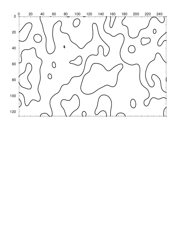
Figure 2: Domain interfaces in a typical two-dimensional model A system.

Numerical simulations of model A were done for flat Euclidean systems of sizes $100\times 100$ and $200\times 200$, with periodic boundary conditions. Forty random order-parameter configurations were generated and evolved by integrating eq. (1) using a standard Forward-in-time/Centered-in-Space Euler integration scheme [7], from $t=0^{+}$ to $t=1000$. The system mesh size $\Delta x$ used was 1, and the time step $\Delta t=0.03$. The results were checked to be independent of system-size. Average computation time required was 8 hours for the 40 runs on an HP735. A typical interface configuration is shown in fig. 2.

Computing ${\vec{K}}$ is very difficult if the bulk description (eq. (1)) is used, as it requires extracting interfaces from the order-parameter configurations by systematically scanning these and finding all interfaces, splining them for smoothness and finally computing ${\vec{K}}$ at regular intervals along an interface. An interface description, which evolves the interfaces directly via an interface equation [8], allows for direct computation of ${\vec{K}}$ and therefore $G_{\!\mbox{\tiny$K$}}(s,t)$, while the runtime can be decreased by a factor of 10 for flat systems and 50 to 100 for the curved (i.e. non-Euclidean) model A [8]. Such a discretized interface description produced results closer to the analytic predictions than did the discretized bulk description (cf. Discussion section), but both yielded otherwise identical results.

The ICAF was computed at several different times during the scaling regime, $t=17$ to $t=300$. The rescaled ICAF, denoted

$${\Xi_{\!\mbox{\tiny$K$}}^{2}(x)}\equiv G_{\!\mbox{\tiny$K$}}^{2}(L_{o}(t)^{-1}s,t),\;\;\;x\equiv L_{o}(t)^{-1}s,$$ (8)

is shown in fig. 3, where the scaling length-scale $L_{o}(t)$

Figure 3: ${\Xi_{\!\mbox{\tiny$K$}}^{2}(x)}$, from bulk configurations at various times. $L_{o}(t)$ was defined as the first zero of $G_{\!\mbox{\tiny$K$}}^{2}(s,t)$.

was arbitrarily defined as the first zero of $G_{\!\mbox{\tiny$K$}}^{2}(s,t)$. The vertical error bars, not shown for clarity, are 0 at the origin and increase roughly linearly to 0.01 in the vicinity of the minimum, then further increase to 0.02 at $s=200$. The error was computed by making an analogy between the curvature ${\vec{K}}$ and magnetization $\vec{m}$ of one-dimensional Ising magnets of different lengths [9]. The error for distance $s$ is then the weighted average of the deviation of each magnet’s value of $\langle m(0)m(s)\rangle$ from the value of $\langle m(0)m(s)\rangle$ for the ensemble of magnets. $G_{\!\mbox{\tiny$K$}}^{2}(s,t)$ corresponds to $\langle m(0)m(s)\rangle$. This was deemed the most reasonable method of error calculation, given the values of ${\vec{K}}$ along an interface, and therefore the statistical error in products of ${\vec{K}}$, are correlated.

3 Discussion

The salient features of the curves in fig. 3 are the nice superposition of the ${\Xi_{\!\mbox{\tiny$K$}}^{2}(x)}$ (within error bars), the power law for $L_{o}(t)$, the negative autocorrelation for $s>L_{o}(t)$, and finally the Gaussian form for distances much smaller than $L_{o}(t)$. The perfect dynamical scaling indicates that the ICAF correctly captures this very important characteristic of model A dynamics, and that the number of runs and system size used give an accurate and reliable measure of $G_{\!\mbox{\tiny$K$}}^{2}(s,t)$. The power law in $L_{o}(t)$ is found through linear regression to be $0.45\pm 0.02$, very close to the theoretical value [10] of 1/2 (the interface description gives a power-law even closer to the analytic prediciton of 1/2, namely $0.48\pm 0.01$, as it is less sensitive to discretization effects). $G_{\!\mbox{\tiny$K$}}^{2}(s,t)$ therefore also captures to a high accuracy the well-known power-law behavior characteristic of model A dynamics.

Over short distances (up to roughly $L_{o}(t)/2$), $G_{\!\mbox{\tiny$K$}}(s,t)$ can be checked to be Gaussian. A Gaussian form for a correlation function was shown by Porod to be a characteristic of fluctuating systems without sharp variations [5]. A plot of $K(s)$ (not shown) indeed looks very much like a snapshot of a one-dimensional fluctuating “membrane”, smooth and without any sharp variations (cf. fig. 2). A first attempt at obtaining an approximate analytical expression for $G_{\!\mbox{\tiny$K$}}^{1}(s,t)$ is exposed here, based on a method developed by T.M. Rogers in his Ph.D. thesis [11], in the context of model B, but never tested numerically.

Consider the model A curvature equations [8] in a flat system:

$${\left({\partial{K}\over\partial t}\right)_{\!\!\alpha}} = {\partial^{2}{K}\over\partial s^{2}}+K^{3}$$ (9)

$${\left({\partial{\sqrt{g}}\over\partial t}\right)_{\!\!\alpha}} = -\sqrt{g}K^{2}$$ (10)

where $s$ is the arclength along an interface, $\alpha$ is a parameterization of the interface in which every point has constant coordinate $\alpha$ (exploiting the fact that the interface moves perpendicularly to itself [8]), and $g$ is the metric on the interface, relating the elements of length in both gauges ($s$ and $\alpha$):

$$\mbox{d}s=\sqrt{g}\;\mbox{d}\alpha.$$ (11)

Now let us make the following mean-field approximation:

$${\left({\partial{\sqrt{g}}\over\partial t}\right)_{\!\!\alpha}} \simeq -\sqrt{g}h(t)$$ (12)

$$h(t) \equiv {1\over L}\int\!\!K^{2}\;\mbox{d}s$$ (13)

where $L$ is the total length of the interface. This approximation becomes exact for circular domains. Furthermore, neglect the cubic term of eq. (9). This term is dominant for circular domains. For convoluted domains, numerical testing indicates $K^{3}$ is comparable to the diffusion term for as many as half the interface points. Therefore, the two approximations work in opposite directions, one becoming exact for circular domains, the other getting better for convoluted domains. On short length-scales, however, convoluted domains are locally circular, but the $K^{3}$ term should be negligible since convoluted domains see their curvature decrease rather than increase. Equation (9) then becomes

$${\left({\partial{K}\over\partial t}\right)_{\!\!\alpha}}={1\over g(t)}{\partial^{2}{K}\over\partial\alpha^{2}}.$$ (14)

Going to Fourier space and making use of a change of variable for time, $g(t)\mbox{d}t^{\prime}=\mbox{d}t$, the integration can now be performed, and the curvature structure factor $\chi_{q}$ obtained:

$$\chi_{q}(t^{\prime})\equiv{1\over N}<K_{q}(t^{\prime})K_{-q}(t^{\prime})>={<K_{q}(0)^{2}>\over N}e^{-2q^{2}t^{\prime}}$$ (15)

where $N$ is the number of points on the interface and $q$ is the wavenumber in the reciprocal space of $\alpha$. Assuming all $K_{q}$ have equal amplitude at $t=0$, a backwards Fourier transform yields

$$G_{\!\mbox{\tiny$K$}}^{1}(\alpha,t^{\prime})=\sqrt{\pi\over 8t^{\prime}}e^{-\alpha^{2}/8t^{\prime}}.$$ (16)

Now $t^{\prime}$ must be found as a function of $t$. This can be done by noting that $h(t)$ is equal to $G_{\!\mbox{\tiny$K$}}^{1}(0,t^{\prime}(t))$, i.e. $h(t)=\sqrt{\pi\over 8t^{\prime}}$. Also,

$$t^{\prime}(t)=\int_{0}^{t}\!\!{\mbox{d}t\over g(t)}.$$

The equation for the metric is therefore

$${\left({\partial{g}\over\partial t}\right)_{\!\!\alpha}}=-2g\sqrt{\pi\over 8}\left(\int_{0}^{t}\!\!{\mbox{d}t\over g(t)}\right)^{-1/2}.$$ (17)

This has $g(t)=t^{-1}/\pi$ as solution, so that $t^{\prime}(t)=\pi t^{2}/2$. From eq. (11), $\alpha=s/\sqrt{g}=s\sqrt{\pi t}$. Substituting in eq. (16),

$$G_{\!\mbox{\tiny$K$}}^{1}(s,t)={1\over 2t}e^{-s^{2}/4t},$$ (18)

which is Gaussian, has time-dependencies consistent with power-law growth in model A dynamics (the amplitude of $G_{\!\mbox{\tiny$K$}}^{1}(s,t)$ has units length squared), and dynamically scales, but does not capture the negative autocorrelations at longer distances. Quantitatively, numerical simulations find the amplitude of the Gaussian to go as $[2(1.1\pm 0.1)t]^{-1}$, in very good agreement with eq. (18), whereas the width is smaller than the prediction (18) by about a factor of two.

Of course, the two approximations that allowed for the calculation of $G_{\!\mbox{\tiny$K$}}(s,t)$ are reasonable only on short length-scales, so it is not surprising that eq. (18) does not capture the dominant wavelength of undulations of the interfaces. Also, all $K_{q}(0)$ were assumed equal. This is obviously wrong, since even at the earliest times the curvature structure factor (the Fourier transform of the $G_{\!\mbox{\tiny$K$}}(s,t)$) shows a well-defined peak at a non-zero $q$ mode. If the correct $\chi_{q}(0)$ is used, then the analytical $G_{\!\mbox{\tiny$K$}}(s,t)$ will have a dip at least at early times. Therefore the strongest approximation may yet lie in the $\chi_{q}(0)$ rather than the mean-field and linearization approximations, though this seems unlikely.

Figure 4: The rescaled curvature structure factors ${\mathscr{S}}_{K}(y)$, as a function of $y\equiv 2\pi L(t)/s$, for the same times as in fig. 3 (joined into one curve for clarity). Fit gives $a=110,b=3/2$ and $c=4/3$ with 3% error.

The most interesting feature of the ICAF is undoubtedly the relatively large negative autocorrelation apparent at distances $s>L_{o}(t)$. Hence the rescaled ICSF ${\mathscr{S}}_{K}(y)$ (Fourier transform of eq. (8)) shows a well-defined peak at a non-zero value of wavevector $y\equiv 2\pi L_{o}(t)/s$, as seen in fig. 4. The functional form can be fitted very nicely to $ay^{b}e^{-cy}$ for $0<y\lesssim 5$, with $a=110\pm 3,b=3/2\pm 0.01$ and $c=4/3\pm 0.04$, though no theoretical justification for this is known to us at present. The maximum of this function occurs at $y=b/c=9/8\pm 0.04$, which is extremely close to 1. The null value of ${\mathscr{S}}_{K}(0)$ stems from the null area under the $G_{\!\mbox{\tiny$K$}}^{1}(s,t)$ curves, itself a direct consequence of

$$\int\!\!{\vec{K}}_{i}\;\mbox{d}s=0$$ (19)

for any interface $i$ (when the system has periodic boundary conditions), a constraint akin to a conservation law. The peak in ${\mathscr{S}}_{K}(y)$ indicates that there is a dominant wavelength for undulations of the interfaces. This dominant spatial mode is a feature which remains as yet either hidden in or inaccessible via the order-parameter structure factor. To our knowledge, it is the first time that it is clearly identified. The closeness of $y$ to 1 also indicates that the first zero of $G_{\!\mbox{\tiny$K$}}^{1}(s,t)$ corrresponds to the dominant spatial oscillation mode for curvature undulations, i.e. the typical arclength distance from a point on the interface at which the curvature changes sign.

The dominant length-scale $L_{o}(t)$ for model A dynamics thus seems to have a different nature than, for instance, that of model B dynamics, whose OPSF itself shows a peak at non-zero wavevector. In the literature on model A and B dynamics one loosely speaks of this dominant length-scale as an average or typical domain size. However the concept of domain size is well defined only when the domains are morphologically disconnected or, if not, if they have a well-defined width. As discussed earlier in this article, model B satisfies this, but for model A only sufficiently off-critical quenches create domains whose bubble morphology lends itself to the definition of a “typical domain size”. The ICAF for model A shows that a dominant length-scale is present in the spatial undulations of the interfaces rather than in the size of the domains. The difference is schematized in fig. 5. We have referred to this dominant length as $L_{o}(t)$, to differentiate it from the degenerate $L(t)$. An interesting question this raises is whether model B interfaces would exhibit not only the dominant length of domain size, but a dominant length of interface undulation as well.

Figure 5: A domain in model A. The width of the OPSF should give an indication of how often domains of size $A$ occur. The line $B$ is what the dominant length-scale is, as given by the ICAF: roughly, the dominant radius of curvature.

The presence of a dominant undulation wavelength implies that model A interfaces may be called “random” only approximately [12], since truly random interfaces have an uncorrelated ICAF rather than the one found here. Several analytical methods developed to derive the scaling function for the OPSF make use of Gaussian assumptions about the order-parameter field as well as the randomness of the interfaces [12]. Though for model A these gaussian assumptions appear to work, the non-gaussian curvature correlations may provide a clue into the break-down of gaussian assumptions for the more complex model B.

An important difference between the OPSF and the ICSF is that the latter distinguishes between the two domain morphologies of model A: bicontinuous for a critical quench, bubble for strongly off-critical quenches. Indeed, the OPSF is qualitatively the same for both morphologies, whereas for the bubble morphology the negative curvature autocorrelations in the ICAF are non-existent: the peak in the ICSF shifts to $y=0$ for sufficiently off-critical quenches. The difference may be due to the absence of phase information in the OPSF.

4 Conclusion

We discussed several features of model A interfacial dynamics via the ICAF (interface curvature autocorrelation function) $G_{\!\mbox{\tiny$K$}}(s,t)$. Two notable characteristics of the ICAF were the gaussian form near $s=0$, and the dip below zero beyond a certain distance. Though time-dependent lengths can be defined from the OPSF, and the existence of a typical and uniquely defined dynamical length $L_{o}(t)$ can be infered from the universality of the OPSF, the peak at zero wavenumber prevents us from uniquely deducing $L_{o}(t)$ and identifying its physical meaning. However the ICAF, through the existence of a zero, or equivalently the ICSF, through the location of its maximum, clearly answers both questions. The scaling length-scale for model A systems is hence in the interface undulations of the domains. This suggests that the scaling length-scale in model A dynamics is of a different nature than the domain-size length-scale of model B dynamics, where the order-parameter is conserved. It is also clear that the OPSF hides some interesting characteristics of model A interface dynamics and its domain morphology. Experimental methods for measuring the interface curvature autocorrelations could become useful in better characterizing the dynamics of some pattern forming systems where sharp interfaces are present.

References

- [1]
- [2] J. D. Gunton, M. S. Miguel, and P. S. Sahni, The dynamics of first-order phase-transitions, in Phase Transitions and Critical Phenomena, edited by C. Domb and J. L. Lebowitz, volume 8, chapter 3, pages 267–466, Academic Press, London, 1983; D. Walgraef, Spatio-temporal pattern-formation: with examples from Physics, Chemistry and Materials Science, Partially ordered systems, Springer-Verlag, New York, 1997.
- [3] P. C. Hohenberg and B. I. Halperin, Rev. Mod. Phys. 49, 435 (1977).
- [4] Y. Oono and S. Puri, Physical Review Letters 58, 836 (1987).
- [5] G. Porod, Small Angle X-ray Scattering, chapter 2, pages 17–51, Academic Press Inc., 111 Fifth Ave., New York, New York 10003, 1982.
- [6] S.M. Allen and J.W. Cahn, Acta Metall. 27, 1085 (1979); M. Grant and J.D. Gunton, Phys. Rev. B28, 5496 (1983).
- [7] W. H. Press, B. P. Flannery, S. A. Teukolsky, and W. T. Vetterling, Numerical Recipes in C: the art of scientific computing, Cambridge Unversity Press, 2nd ed. edition, 1992.
- [8] O. Schönborn and R. C. Desai, Kinetics of phase ordering on curved surfaces, submitted (1998); O. Schoenborn, Phase-ordering kinetics on curved surfaces, Ph.D. thesis, Dept. of Physics, University of Toronto, 60 St-George St., Toronto, ON, Canada, M5S 1A7 (1998).
- [9] H. Müller-Krumbhaar and K. Binder, Journal of Statistical Physics 8, 16 (1973).
- [10] A. Bray, Adv. Phys. 43, 357 (1994).
- [11] T.M. Rogers, Domain Growth and Dynamical Scaling during the late stages of Phase Separation, Ph.D. thesis, Dept. of Physics, University of Toronto, 60 St-George St., Toronto, ON, Canada, M5S 1A7 (1989).
- [12] C. Yeung, Y. Oono, and A. Shinozaki, Physical Review E 49, 2693 (1994); H. Toyoki, Physical Review B 38, 11904 (1988); T. Ohta, D. Jasnow, and K. Kawasaki, Phys. Rev. Lett. 49, 1223 (1982).