Phase Diagram of High-T_c Superconductors from a Field Theory Model

Abstract

The renormalization group approach to correlated fermions is used to determine the phase diagram of the oxide cuprates modeled by the $t-t^{\prime}$ Hubbard model at the Van Hove filling. Spin–dependent interactions give rise to instabilities corresponding to ferromagnetic, antiferromagnetic and d-wave superconducting phases. Antiferromagnetism and d-wave superconductivity arise from the same interactions, and compete in the same region of parameter space.

I Introduction

Ten years after their discovery, the study of the high-T_c superconductors[1] continues being a major puzzle for theoreticians. Despite the accumulation and accuracy of experimental data now at hand, the theoretical situation has not improved much since the early days of high-T_c, and many of the models proposed then are still at work with very few new ideas available [2]. The problem is tough because the cuprates are a system of highly correlated electrons interacting at an intermediate to strong coupling regime.

The paradigm of the metallic behavior, the Landau Fermi liquid theory, [3] fails to describe the “normal” state above the critical temperature, and the BCS theory of superconductivity even in its strong coupling formulation can not account for the high temperatures reached by these compounds. It is clear that, even if phonons do play some role, we must look for a pairing attraction of a different nature – electronic or magnetic – in the cuprates.

As it is known, all the copper-oxide high-T_c materials come from an insulating antiferromagnetic “father” compound (a Mott insulator) which becomes superconducting upon either electron or hole doping. This metal-insulator transition inspired Anderson [4] to propose the two-dimensional Hubbard model close to half filling as a starting point to model the correlations in the cuprates. The importance of antiferromagnetic fluctuations led to the early proposal of the t-J model [5]. Most of the theoretical efforts in the field are devoted to study the various extended Hubbard models with the available techniques numerical or perturbative [6]. The issue of whether or not the Hubbard model supports superconducting instabilities and at which range of temperature and doping is one of the most active areas of research on the field.

One of the most prominent features in the physics of the cuprates is the many different energy scales where interesting phenomena occur. From the beginning it was clear that the pair formation takes place at a different energy scale than the superconducting transition [7]; recent – as well as early – photoemission experiments on hole-doped materials have confirmed the existence of a pseudogap in the underdoped regime (below the doping at which the highest transition temperature occurs or optimal doping) at an energy scale much higher than the transition temperature. On the other hand we have the various magnetic scales. In order to reach the physics responsible for a given phenomenon, we must be able to integrate away irrelevant degrees of freedom.

A related feature is the existence of different kinds of coexisting and possibly competing instabilities within a certain range of the parameters. In particular, one of the proposed pairing mechanism in the cuprates relays on the competing spin density-wave and superconducting instabilities, the pairing would be induced by an incipient instability of the spin density-wave type. Besides, weak coupling approaches to the Hubbard model have shown that it is more likely to develop a spin-density-wave instability than superconductivity at half-filling [8, 9, 10]. Inclusion of a next-to nearest neighbors coupling, the so–called Hubbard t–t’ model, enlarge the possible instabilities of the system and opens the door for d–wave pairing instabilities.

The renormalization group (RG) approach to interacting fermions proposed in [11, 12] is an optimal framework to deal with this problem.

In recent years great effort has been devoted to study the role of Van Hove singularities (VHS) in two-dimensional electron liquids [13, 8, 9, 14, 15, 16, 17, 18]. Most part of the interest stems from the evidence, gathered from photoemission experiments, that the hole-doped copper oxide superconductors tend to develop very flat bands near the Fermi level [19, 20]. Near a Van Hove singularity the fermion density of states diverges so even very weak interactions can produce large effects. A Van Hove singularity is a saddle point in the dispersion relation of the electron states $\varepsilon({\bf k})$. In its vicinity, the density of states diverges logarithmically in two dimensions, and shows cusps in three dimensions. The logarithmic divergence leads to a singular screening of the interactions, in the same way as for the 1D Luttinger liquid [21].

Van Hove singularities have been largely ignored in the past mostly because they do not arise in three dimensions where they can be integrated to give a finite density of states. Their influence in two–dimensional systems was minimized on the following basis: under a theoretical point of view it was argued that i) they are isolated points in a Fermi line, hence a zero measure set; ii) the shape of the Fermi surface is a relevant parameter in the RG sense that gets renormalized by the interaction hence fixing the Fermi surface at a VHS appeared as a fine-tunning condition; finally, there was no anomalous behavior whose explanation could be helped by invoking the existence of VHS. It has also been argued that disorder effects would spoil the d–wave pairing predicted by the Van Hove model.

The physics of the cuprates has changed the above points in various respects. First of all, there are photoemission spectra showing the existence of very flat bands close to the Fermi level in most underdoped cuprates what suggests a Fermi surface very close to a VHS. Then, different approaches including a RG study [16] have shown that the Fermi surface of the two dimensional Hubbard model has a tendency to be pinned near the VHS. It was shown in [16] that for open systems, the renormalization of the chemical potential is such that the VHS filling is an attractive fixed point of the renormalization group. For a range of initial dopings close to the singularity the renormalized system flows towards it. This result obviates the major theoretical objection refering the fine tunning. Finally, it has been shown in a recent publication [22], that disorder effects may reduce but do not eliminate the electronic pairing induced by the VHS’s.

Even if the VHS’s are not responsible for the normal state anomalies of the cuprates, it is worth studying them as their presence can substantially alter the behavior of any model. In the case of the Hubbard model on the square lattice, the existence of two independent VHS’s also provides new scattering channels for the low-energy modes what reinforces the possibility of anisotropic pairing of electronic origin.

In addition to the phenomenological interest in condensed matter physics, the study of the Hubbard model filled up to the level of the VHS, poses very interesting questions to the RG procedure applied to a quantum statistical model which would not arise in a standard renormalizable quantum field theory and that deepens our understanding of the RG physics.

In previous works [16, 17] a superconducting instability was found in a simplified model of VHS with two singularities and spin-independent interactions. In this paper we look for the instabilities of the repulsive $t-t^{\prime}$ Hubbard model, filled up to the level of the Van Hove singularity, following the RG program of Refs. [11, 12]. Preliminary results on this work can be found in [23].

The organization of the paper is as follows. First we introduce the model as comes from the continuum limit of the one-band Hubbard model, identify the VHS’s and classify all possible couplings. Next we briefly review the RG procedure as applied in condensed matter physics. In the next section we study the renormalization of the bare couplings for the case of a local interaction. Section 4 is devoted to the physical implications of this work. We study the response functions of the system and get the phase diagram that they lead to. Section 5 contains a summary of the results, discussions and future work.

II The model

The RG properties of the Hubbard model at the Van Hove filling have been presented in [16, 17]. We will here review its most prominent features. As it is known, the Hubbard model was designed to reproduce the Mott transition [24] found in some metals. It is originally defined in a lattice by the hamiltonian:

$$H_{Hub}=-B\sum_{<ij>,\sigma}c^{+}_{i,\sigma}c_{j,\sigma}+U\sum_{i}n_{i,\uparrow}n_{i,\downarrow}\;\;\;,$$ (1)

where B is the band width without correlation, that is, in the absence of U, U is the intra-atomic energy, $\;U=<e^{2}/r_{12}>\;\;,\;\;c^{+}_{i,\sigma}\;$ creates an electron at site $i$ with spin $\sigma$, and $n_{i}$ is the particle density at site $i$, $n_{i,\uparrow}=c_{i,\uparrow}^{+}c_{i,\uparrow}$. Hubbard showed that with this hamiltonian the spectrum of quasiparticles splits into two bands which overlap when the lattice spacing $a$ is $\;a<a_{0}=B/U=1.15\;$ describing an antiferromagnetic metal while it describes an antiferromagnetic insulator for larger values of $a$. Nagaoka pointed out that the system would only be insulating exactly at half filling when the number $n$ of electrons equals the number of lattice sites being metallic for any other filling (doping). He also noticed that it would show ferromagnetic behavior in the limit of small values of $B/U$.

We shall here use the simple one-band Hubbard model which has proven to be a good starting point for the description of the band properties of most cuprate materials. In a tight-binding approximation, (1) is written as

$$H=\sum_{{\bf k},\sigma}\varepsilon({\bf k})\;c^{+}_{{\bf k},\sigma}c_{{\bf k},\sigma}\;+\;U\sum_{i}n_{{\bf k},\uparrow}n_{{\bf k},\downarrow}\;\;\;.$$

When defined on a square lattice which is appropriate for the $Cu-O$ planes of the cuprates, and for nearest–neighbor hoping, the dispersion relation $\varepsilon({\bf k})$ is

$$\varepsilon({\bf k})=-2t\;[\cos(k_{x}a)+\cos(k_{y}a)]\;\;\;,$$

where $a$ is the lattice constant. The Fermi surface at half filling has a diamond shape with saddle points located at the four corners of the Brillouin zone $(0,\pm\pi)\,,\,(\pm\pi,0)\;$. It shows perfect nesting [11], i.e. two parts of the Fermi surface run parallel over an entire edge separated by a common vector ${\bf Q}$. This nesting induces a peak in the joint density of states

$$J({\bf Q})=\int d^{2}kN(\varepsilon_{{\bf k}})N(\varepsilon_{{\bf k}+{\bf Q}})$$

even when the individual single particle density of states (DOS) is featureless. In contrast, near a VHS, the DOS has already a strong peak such that if ${\bf Q}$ joins two VHS’s, a large peak in J is assured. This will show up in the spin or charge susceptibilities to be discussed later.

The global nesting property is not observed in the photoemission experiments. The saddle points observed in [19] can be incorporated into the metallic regime of the Hubbard model by introducing a next-nearest neighbor interaction [26] which modifies the dispersion relation as

$$\varepsilon({\bf k})=-2t\;[\cos(k_{x}a)+\cos(k_{y}a)]-2t^{\prime}\cos(k_{x}a)\cos(k_{y}a)-\mu-2t^{\prime}\;\;\;,$$ (2)

where we have included the chemical potential $\mu+2t^{\prime}\;$.

FIG. 1.: Different shapes of the Fermi line for the $t-t^{\prime}$ Hubbard model about the Van Hove filling.

Different constant-energy lines for (2) are shown in fig. 1. $\mu=0$ corresponds to the Fermi surface sitting at the Van Hove singularities denoted A and B in the figure. The $t^{\prime}$ interaction, besides destroying the perfect nesting of the Hubbard model, allows to fit the phenomenology observed in the hole-doped cuprates for which the Fermi level lies close to the saddle point at a doping of 0.15 to 0.25. $t^{\prime}$ controls the shape and curvature of the Fermi surface. For the hole-doped materials, $t^{\prime}<0$ and in all cases, $t^{\prime}<t/2$. The suppression of conventional nesting greatly reduces the possibility of a charge density wave (CDW) or a spin density wave (SDW) instability while retaining a strong superconducting (SC) instability [25, 26]

We construct a continuum model by assuming that for fillings such that the Fermi line lies close to the singularities, the majority of states participating in the interactions will come from regions in the vicinity of the points A, B of fig. 1. We then perform a Taylor expansion of (2) around A and B and shift the origin of momenta to obtain the following dispersion relation to be used as the kinetic term in the field theory model:

$$\varepsilon_{A,B}({\bf k})\approx\mp(t\mp 2t^{\prime})k_{x}^{2}a^{2}\pm(t\pm 2t^{\prime})k_{y}^{2}a^{2}$$ (3)

where the momenta $k_{x},k_{y}$ meassure small deviations from $A,B$. As we see, the parameter $t^{\prime}$ controls the angle between the two separatrices of the hyperbolae of constant energy, $\varphi=2\arctan[(t+2t^{\prime})/(t-2t^{\prime})]$.

Knowing that scattering among the two singularities plays an essential role in enhancing the superconducting instabilities of the system, we will map the problem onto a model of electrons with two flavors A and B denoting the electrons close to each of the VHS’s. Interactions will take place among electrons of the same and of different flavors. We shall apply RG techniques to the model based on the fact that our physical system contains two natural energy scales. One is the bandwidth of the order of some electron volts and the other is the temperature or the energy of the elementary excitations over the vacuum, several orders of magnitude smaller. We will then establish an energy cutoff of the order of the band width and renormalize it towards the Fermi surface $\varepsilon({\bf k})=0$.

In the RG approach we write down a low-energy effective action which is scale invariant at tree level and check where is it driven by the marginal and relevant perturbations. We will obtain RG equations by integrating virtual states of two energy slices above and below the Fermi level in an energy range given by the cutoff $E_{c}$, $E_{c}-|dE_{c}|<|E|<E_{c}$. We are interested in the scaling behavior of the interactions and correlations under a progressive reduction of the cutoff, which leads to the description of the low-energy physics about the Fermi level.

Integrating over a differential energy slice in the computation of a given vertex function allows to extract the differential equation that governs the scaling of the given coupling. The procedure should be equivalent to the one used in quantum field theory where the integration is performed over the entire cutoff range and the derivative with respect to the cutoff is taken afterwards. In our case, the differential approach has the advantage that allows us to discuss scaling properties without getting too close to the Fermi line ($E_{c}=0$) where single–particle properties can become unreliable. We will insist on that later in connection with the study of the response functions of the system.

Let us now proceed to the building of the model. The free part of the low-energy effective action in momentum space is

$$S_{0}=\int d\omega d^{2}k\sum_{\alpha,\sigma}\;[\omega-\varepsilon_{\alpha}({\bf k})]\;a^{+}_{\alpha,\sigma}({\bf k},\omega)a_{\alpha,\sigma}({\bf k},\omega)$$ (4)

where $a_{\alpha,\sigma}\;\;(a^{+}_{\alpha,\sigma})$ is an electron annihilation (creation) operator and $\alpha$ labels the Van Hove point. The scaling behavior of (4) has been analyzed in detail in [17]. It is clear that it is scale-invariant provided that under a rescaling of the energy $\;\omega\rightarrow s\omega\;\;,\;\;s<1\;\;$, we have

$${\bf k}\rightarrow s^{1/2}{\bf k}\;\;\;,\;\;\;a_{\alpha,\sigma}({\bf k},\omega)\rightarrow s^{-3/2}\;a_{\alpha,\sigma}({\bf k},\omega)\;\;\;.$$ (5)

Next we discuss the interaction. In order to mimic a continuum analogue of the Hubbard interaction U in (1) we will write down in the effective action an interaction of current–current type among currents of opposite spin:

$$S_{{\rm int}}=-\frac{U}{2}\int d\omega d^{2}k\;\left(\rho_{\uparrow}({\bf k},\omega)\>V({\bf k})\>\rho_{\downarrow}(-{\bf k},-\omega)\right)$$ (6)

where $\rho_{\sigma}({\bf k},\omega)$ are the Fourier components of the density operator

$$\rho_{\sigma}({\bf k},\omega)=\frac{1}{(2\pi)^{3}}\int d\omega_{p}d^{2}p\;a^{+}_{\sigma}({\bf p}-{\bf k},\omega_{p}-\omega)a_{\sigma}({\bf p},\omega_{p})$$ (7)

In the spirit of the Wilson effective action, U encodes all the possible couplings compatible with the symmetries of the problem that are marginal at tree level with the only extra requirement of been among currents of opposite spin. We will not allow spin flip interactions. As mentioned before, the interaction parameter $U$ of the Hubbard model represents a point-like interaction of the fermions in the lattice. The direct interpretation of it in the continuum limit would be a delta–function interaction in real space, i.e. a constant $V({\bf k})$ in Fourier space, or, else, we can interpret $U$ as a short–range interaction between the fermions having a finite support. It turns out that this two possibilities give rise to differences in the diagrammatics but do not alter the physical realization of the model as we shall later see.

Here we will classify and analyze all spin-dependent local interactions fixing $V({\bf k})=1$. From the scaling behavior (5) we see that for this choice, the interaction is a marginal operator. Any analytical function $V({\bf k})$, once expanded in powers of ${\bf k}$, would leave the constant term as a marginal operator and the rest would be irrelevant operators. Notice that an interaction of the type discussed above, say $V({\bf r})=1/r^{2}$ could also arise as the continuum limit of a local Hubbard interaction. In momentum space this is a logarithmic interaction of the kind that has been invoked before in the context of the Van Hove model [17] as a cure for the squared logarithms that appear in the renormalization of some diagrams. Such a logarithmic interaction is also scale invariant at tree level and should, in principle, be taken into account. The non–local character of the $1/r^{2}$ interaction would exclude it from appearing in a quantum field theory analysis where the locality of the operators is linked to the property of causality. In a non–relativistic model this consideration does not take place. We are then confronted to study the renormalization of two different operators with the same quantum numbers and the same scaling dimensions. We shall take them as independent and will try not to mix them upon renormalization. We will come to that later.

The RG analysis for the case of a spin-independent interaction with a finite support in $k$-space and within a single singularity was done in detail in [17] while the spin-independent case but allowing intersingularity scattering was studied in [16]. The analysis presented here is the most complete one performed within the RG and should show all the possible instabilities of the repulsive t–t’ Hubbard model for local interactions at moderate values of U.

At this point it is worth noticing that the marginal character of the four–fermion interaction in the two–dimensional Van Hove model proposed here, marks already a difference with the isotropic Fermi liquid model in two dimensions. There, the four–fermion interaction is generically irrelevant being marginal only for processes with a particular kinematics [11]. This is due to the constraint that momentum conservation imposes on the different processes, very severe in the case of an isotropic Fermi line. In particular only forward and backward scattering gives rise to a –finite– renormalization of the four–Fermi interaction in the standard model. The reason is that these processes realize a kind of “dimensional reduction” and have the naive scaling dimensions of the D=1 situation.

In the Van Hove model, the four–Fermi coupling is generically marginal due to the particular scaling of the integration meassure (5) dictated by the free dispersion relation. Although in the Fermi–liquid case the integration messure also has the naive dimension of the D=1 case, there it is due to the kinematical decomposition of the momenta into perpendicular and parallel to the Fermi line and the choice that only the perpendicular component scales with the energy. In the Van Hove case, the dimensional reduction of the integration meassure has its origin in the particular form of the Fermi line at the singularity very much as happens in D=1.

Next, unlike what happens in the marginal couplings of the Fermi liquid, the renormalization of the couplings in the Van Hove model is nontrivial due to the logarithmic divergence of the density of states dictated again by the dispersion relation. All that will become clear in what follows.

The complete classification of the interactions including the two flavors A and B follows exactly the one that occurs in the g-ology of one–dimensional systems [21, 27] where the role of the two Fermi points is here played by the two singularities. We will see nevertheless that the one–dimensional parallelism stops at the classification level as kinematical constraints in two dimensions make the evolution of the couplings very different from that of one-dimensional systems.

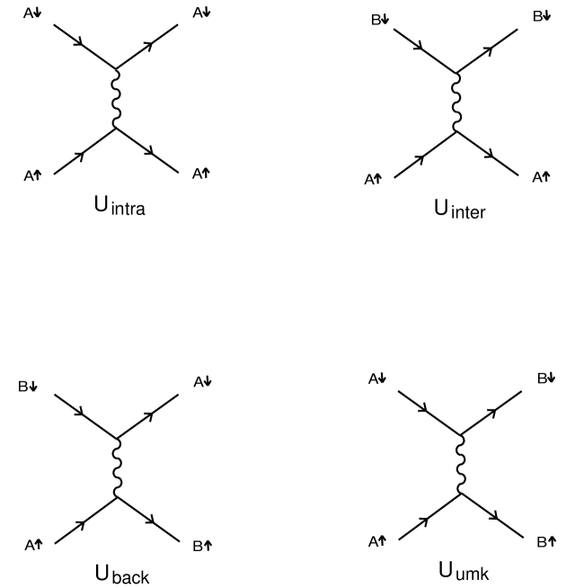
FIG. 2.: Different interaction terms arising from the flavor indices A and B .

In general there are four types of interactions that involve only low-energy modes. They are displayed in fig. 2 where the interaction is represented by a wavy line to clarify the process it refers to. In the model that we are considering, the wavy lines should be shrank to a point giving rise to couplings typical to the $\Phi^{4}$ quantum field theory. The spin indices of the currents are understood to be opposite in all cases. The interactions are classified as follows. Intrasingularity interactions , $U_{{\rm intra}}$ occur around the same singularity. Low energy implies for that case low momentum transfer, the logarithmic singularities will occur at zero momentum transfer.

Intersingularity interactions occur when a type A current exchanges momenta with a type B current (or viceversa) as displayed in fig. 2. The momenta exchanged in these processes is again low.

A different kind of process occur when two electrons close to the singularities A, B, are excited to the vicinity of the opposite singularity. This is a low–energy process that involves a momentum transfer of order ${\bf Q}$, the vector joining the two singularities, and the logarithmic singularities will appear for ${\bf Q}=(\pi,\pi)$. The corresponding graph is called $U_{{\rm back}}$

The last interaction called $U_{{\rm umk}}$ deserves some comment. It describes a process in which two electrons of opposite spin near the singularity $A$ jump together to the singularity $B$. In the continuum, due to momentum conservation, such a process would not be allowed or else would have a very high energy. In the presence of a lattice however the momentum needs only to be conserved modulo one vector of the reciprocal lattice. In the $U_{{\rm umk}}$ interaction, the momentum transfer ${\bf P}=(2\pi,2\pi)$ coincides with a lattice vector and is such that $\varepsilon({\bf k}+{\bf P})=-\varepsilon({\bf k})$. Such interaction processes are called umklapp. As we will see, they play a major role in our model as they are responsible for the antiferromagnetic and superconducting instabilities.

III Renormalization of the couplings.

The interaction $V({\bf k})$ can be renormalized to second order in perturbation theory by the diagrams despicted in fig. 3 where the spin indices have been omited. The bare couplings of fig. 2 are by now to be considered as vertex functions $i\Gamma({\bf k},\omega)$ i.e. the part of the interaction without the external legs.

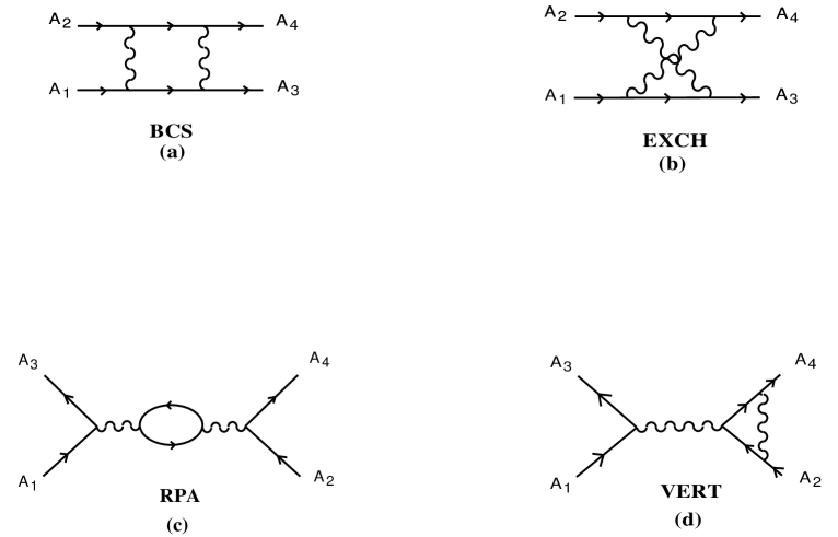
FIG. 3.: Diagrams contributing to the one-loop order correction to the interaction potential.

They are two types of corrections in fig. 3: direct (BCS) and exchange (EXCH) particle–particle interactions (fig. 3 (a), (b)), particle–hole interactions called RPA in fig. 3 (c), and vertex corrections called VERT in fig. 3 (d).

Once the interactions are shrinked to a point, they turn into the diagrams despicted in fig. 4 which are the ones to be computed in the one-loop calculation. We must keep in mind that, according to fig. 3, the correction induced by the BCS diagram (fig. 3 (c)) has a minus sign relative to the others as it carries a closed fermion loop.

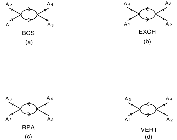
FIG. 4.: Diagrams of fig. 3 with the interaction shrinked to a point.

The first thing to notice from fig. 4 is that the particle–hole diagrams (c), (d), when inserted into a coupling function, will provide exactly the same correction but with an opposite sign due to the fact that there is a closed fermionic loop in the original RPA coupling which is absent in the diagram called VERT. This cancellation that, to our knowledge, was first noticed in the original work of ref. [29], occurs to all orders in perturbation theory. It has important consequences as it elliminates the RPA graphs which are the typical screening processes for repulsive interactions considered in most of the papers. It should be noticed however that the cancellation only takes place for contact interactions of the Hubbard type. Any k-dependence of the interaction would restore the prevalence of the RPA graphs for small momentum transfer. Moreover, diagrams (c) and (d) of fig. 3 do not exist if the interaction is restricted to currents of opposite spins as in our case. In what this work is concerned, we are then restricted to study the vertex corrections provided by the particle–particle diagrams of fig. 4 (a), (b).

The BCS diagram of fig. 4 (a) is only singular for definite values of the external momenta and hence is not to be taken into account in the renormalization of the vertex functions. Nevertheless, it will play an important role in the study of the instabilities of the system through the response functions to be done in the next section. The analysis of the renormalization induced by this coupling is similar to the one done for an isotropic Fermi line [11]. The resulting logarithmic singularity is of the form $\log\;({\bf k_{1}}+{\bf k_{2}})$ which diverges only for the BCS kinematics, i.e. if the total incoming momentum adds to zero. In the differential approach that we are using, this is best seen graphycally as despicted in fig. 5.

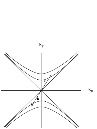
FIG. 5.: Two energy slices used in the computation of the BCS graph.

Two energy integration slices contributing to the computation of the BCS graph are shown in fig. 5. It is clearly seeen that, unless the total momentum of the incoming particles adds to zero, the area of the intercept of the two bands, which meassures the cutoff dependence of the diagram is of order $(dE_{c})^{2}$. This is different from what happens in one dimension, where the BCS graph contributes to the renormalization of all quartic couplings. In the Van Hove model, the divergence of the BCS graphs at the kinematical singularity has a logarithm squared singularity but the kinematical dependence remains the same.

This leaves us with the diagram of fig. 4 (b) as the only contribution to the renormalization of the couplings at the one loop level. In terms of the fermion propagator $G^{(0)}_{\sigma}({\bf k},\omega)$ for each respective spin orientation, the vertex function at the one loop level $\>i\Gamma^{(2)}({\bf k},\omega)\>$ is computed as

$$i\Gamma^{(2)}({\bf k},\omega)=-\frac{U^{2}}{(2\pi)^{3}}\int_{-\infty}^{\infty}d\omega_{q}\int^{\Lambda}d^{2}q\sum_{\sigma}G^{(0)}_{\sigma}({\bf q}+{\bf k},\omega_{q}+\omega)G^{(0)}_{\sigma}({\bf q},\omega_{q})\;\;\;,$$ (8)

where the momentum transfer in the vertices is such that $\Delta k_{2\rightarrow 3}=\Delta k_{1\rightarrow 4}$. The momentum integrals are restricted to modes within the energy cutoff, $|\varepsilon_{\alpha}\;({\bf k})|\leq E_{c}$ as the ones represented graphycally in fig. 5 where now one of the slices is, as before, in the particle zone and the second one is at the empty side of the Fermi sea. It can be seen graphycally that the intercept of the two slices for this case has always a linear contribution in $E_{C}$ for small momentum transfer.

The fermion propagator to be used in our model is

$$G^{(0)}_{\sigma}({\bf q},\omega_{q})=\frac{1}{\omega_{q}-\varepsilon({\bf q})+i\epsilon\>\rm{sgn}\>\epsilon_{q}}\;\;\;.$$ (9)

Near a Van Hove point, e.g. $\;A=(\pi,0)\;$, we have

$$\varepsilon({\bf q})=-u_{0}\;(q_{x}^{2}-\beta^{2}\;q_{y}^{2})\;\;,$$ (10)

where

$$u_{0}=2(t+2t^{\prime})a^{2}\;\;\;,\;\;\;\beta^{2}=\frac{t-2t^{\prime}}{t+2t^{\prime}}\;\;\;.$$

Perfect nesting will be absent as long as $\beta$ stays different from one ($t^{\prime}\neq 0$).

Due to the sign of the imaginary part in (9), the poles of the two propagators will be in a different half–plane only if the particles involved come from opposite sign regions of $\varepsilon({\bf q})$. This means that the virtual states in the loop always involve a particle (hole) on the filled $\varepsilon({\bf q})\;>0$ (empty) side of the Fermi sea, been scattered to a hole $\varepsilon({\bf q}+{\bf k})\;<0$ (particle) on the opposite region.

Due to the presence of the two flavors, two types of loops (polarizations) have to be computed: particle-hole processes around the same singularity and processes in which the particle and the hole live near two different singularities, the last involve a momentum transfer of order ${\bf Q}=(\pi,\pi)\;$.

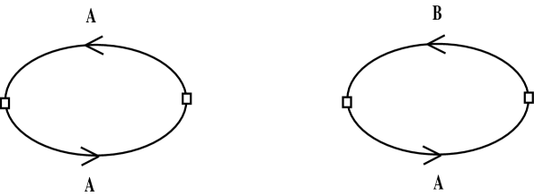
FIG. 6.: The two polarizabilities used in the paper.

The two polarizabilities shown in fig. 6 have been computed in [16, 17]. Their dependence on the cutoff is

$${\rm Re}\>\Gamma^{(2)}_{{\rm intra}}(\omega)\sim\frac{c}{2\pi^{2}t}U^{2}\log(E_{c}/\omega)$$ (11)

$${\rm Re}\>\Gamma^{(2)}_{{\rm inter}}(\omega)\sim\frac{c^{\prime}}{2\pi^{2}t}U^{2}\log(E_{c}/\omega)\;\;,$$ (12)

where

$$c\equiv 1/\sqrt{1-4(t^{\prime}/t)^{2}}\;\;\;,\;\;\;c^{\prime}\equiv\log\left[\left(1+\sqrt{1-4(t^{\prime}/t)^{2}}\right)/(2t^{\prime}/t)\right]\;\;\;.$$ (13)

As mentioned before, the logarithmic divergences of the vertex functions here are due to the divergent density of states near the Van Hove singularity. The same graphs do not have a logarithmic dependence on the cutoff in the case of the two–dimensional isotropic model for generic values of the momenta. Only forward or backward scattering at zero momentum are enhanced in that case [3]. The bare susceptibility defined at this order in perturbation theory as $\chi({\bf q})=\Gamma({\bf q},\omega=0)$, diverges at both ${\bf q}=0$ where it coincides with the density of states, and at ${\bf q}=(\pi,\pi)$, due to intersingularity scattering. The latter has a squared logarithm singularity when the Fermi surface is nested, $t^{\prime}=0$, a situation that was treated in ref. [17]. This squared logarithm singularity is cutoff to a usual logarithm when $t^{\prime}\not=0$.

The corrections to each of the couplings of fig. 2 are obtained by “opening up” the graph and inserting the polarizabilities in such a way that the resulting graph is of the type of fig. 4 (b) and the vertices are made up of the tree–level interactions of fig. 2.

Let us first discuss the behavior of any coupling, say $U_{{\rm inter}}$. $U_{{\rm inter}}$ is renormalized by the diagrams shown in fig. 7.

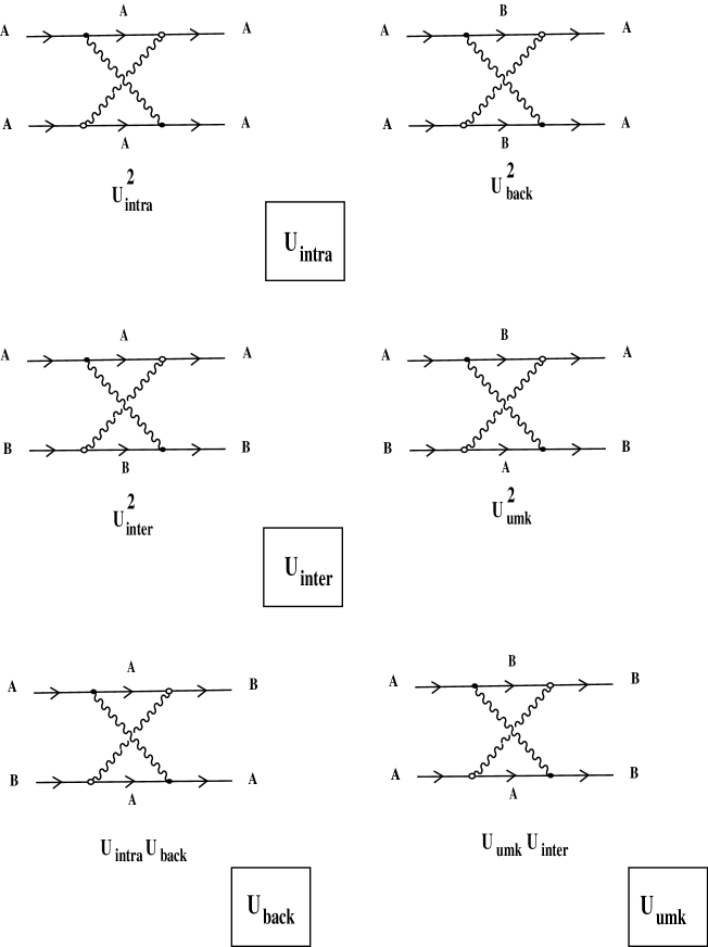
FIG. 7.: Renormalization of the different couplings described in the text.

Adding up the one–loop correction to the bare coupling we find the vertex function at this order

$$\Gamma_{{\rm inter}}({\bf k},\omega)=U_{{\rm inter}}+\frac{c^{\prime}}{2\pi^{2}t}(U_{{\rm inter}}^{2}+U_{{\rm umk}}^{2})\log\left|\frac{E_{c}}{\Lambda}\right|\;\;\;E_{c}<\Lambda\;\;.$$ (14)

Following the usual procedure [28], we shall define the dressed coupling constant at this level in such a way that the vertex function be cutoff independent what implies the RG equation

$$E_{c}\frac{d\;U_{{\rm inter}}(E_{c})}{d\;E_{c}}=\frac{c^{\prime}}{2\pi^{2}t}(U_{{\rm inter}}^{2}+U_{{\rm umk}}^{2})\;,$$ (15)

were the polarizability involved is the interparticle polarizability and the sign of the beta function is positive as corresponds to the “antiscreening” diagram of fig. 3 (b). The same equation (15) is obtained by integrating over a differential energy slice as we mentined earlier.

The growth of the coupling will eventually produce an instability in the system to be discussed later.

We now apply the same procedure to the rest of the couplings. The diagrams that induce non–trivial renormalization are represented graphycally in fig. 7, where the spin polarizations of the currents have been omited and should be seen as opposite in all cases. We obtain the following set of coupled differential equations for the couplings:

$$E_{c}\frac{\partial U_{{\rm intra}}}{\partial E_{c}} = \frac{1}{4\pi^{2}t}c\left(U_{{\rm intra}}^{2}+U_{{\rm back}}^{2}\right)$$ (16)

$$E_{c}\frac{\partial U_{{\rm back}}}{\partial E_{c}} = \frac{1}{2\pi^{2}t}c\left(U_{{\rm intra}}U_{{\rm back}}\right)$$ (17)

$$E_{c}\frac{\partial U_{{\rm inter}}}{\partial E_{c}} = \frac{1}{4\pi^{2}t}c^{\prime}\left(U_{{\rm inter}}^{2}+U_{{\rm umk}}^{2}\right)$$ (18)

$$E_{c}\frac{\partial U_{{\rm umk}}}{\partial E_{c}} = \frac{1}{2\pi^{2}t}c^{\prime}\left(U_{{\rm inter}}U_{{\rm umk}}\right)$$ (19)

where $c,c^{\prime}$ are the prefactors of the polarizabilities at zero and ${\bf Q}$ momentum transfer, respectively given in (13).

The RG equations (16)-(19) describe a flow that drives the couplings to large values as the cutoff is sent to the Fermi line. The growth of the couplings is to be understood as the tendency of the system to flow towards a strongly coupled system with different physical properties. Although the RG looses predictive power as we approach the frequency where the couplings diverge, the physical properties of this regime can be qualitatively studied by means of the response functions as will be described in the next chapter.

We will compute the flow dictated by the RG equations starting with all the couplings set to a common value $U$. This assumption is not relevant in what concerns the subsequent flow as long as the couplings start being positive. It can be easily seen that the flow described by (16)(17) is attracted towards a region in which $U_{intra}\sim U_{back}$ and that both diverge at the same critical scale. The same applies to $U_{inter}$ and $U_{umk}$. The only relevant feature may be a significant difference between $U_{intra}$ and $U_{inter}$ at the starting point of the RG flow. Under the change of variables

$$U_{1\pm}=U_{intra}\pm U_{back}\;\;\;,\;\;\;U_{2\pm}=U_{inter}\pm U_{umk}\;\;\;,$$

(16)–(19) turn into

$$\frac{\partial U_{1\pm}}{\partial\log E_{C}}=\frac{c}{2\pi^{2}t}U_{1\pm}^{2}\;\;\;;\;\;\;\frac{\partial U_{2\pm}}{\partial\log E_{C}}=\frac{c^{\prime}}{2\pi^{2}t}U_{2\pm}^{2}\;\;\;,$$

what shows that the above initial difference may be reinterpreted in terms of an equivalent model with $U_{intra}=U_{inter}$ and different values of the constants c and c’.

Under the initial condition that all couplings are equal to $U$ it is clear that $U_{{\rm intra}}=U_{{\rm back}}$ and $U_{{\rm inter}}=U_{{\rm umk}}$, all along the flow.

A scaling analysis of the equations (16)–(19) trading the cutoff dependence by a dependence on the momentum at which we are probing the system, allows us to write down the following equations

$$U_{{\rm intra}}(\omega) = \frac{U}{1+U\>c/(2\pi^{2}t)\>\log(\omega/E_{c})}$$ (20)

$$U_{{\rm inter}}(\omega) = \frac{U}{1+U\>c^{\prime}/(2\pi^{2}t)\>\log(\omega/E_{c})}$$ (21)

The flow of the two couplings is despicted in fig. 8.

FIG. 8.: Schematic view of the flow of the couplings discussed in the text.

We shall end this section with the discussion of a fine point that arises in the renormalization of the couplings at the one loop level. In the study of the one–dimensional case, most references make a distinction between couplings among currents with different spin orientation as the one considered here, called $U_{\perp}$, and currents with the same spin orientation, called $U_{\parallel}$. We have neglected the last set because we made the decision of discussing a continuum model as close as possible to the original Hubbard model (1). We could have, in principle, enlarged the model with the inclusion of two extra couplings of the type $U_{{\rm inter}\parallel}$ and $U_{{\rm back}\parallel}$. The other two parallel couplings $U_{{\rm intra}\parallel}$ and $U_{{\rm umk}\parallel}$, would be forbidden at tree level by the Pauli exclusion principle and the point–like character of the interaction.

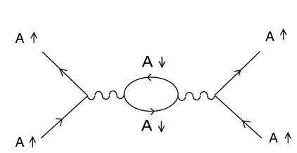
FIG. 9.: A diagram which generates a parallel coupling at one loop level.

The point is that by joining up the external legs of two couplings, say of the $U_{{\rm intra}\perp}$ type as shown in fig. 9 , we can generate at one loop a parallel coupling of the type $U_{{\rm intra}\parallel}$ not present in the tree level lagrangian. Generation of new couplings at higher orders in perturbation theory is usually protected in quantum field theory (QFT) by symmetry principles — unless the theory is non–renormalizable — but it is a well known phenomenon in condensed matter systems responsible for physically relevant effects such as the Kondo effect or the attractive coupling among electrons induced by the electron–phonon interaction. The usual treatment in QFT would be to add to the lagrangian at tree level the coupling whose renormalization is being established at one loop. We can not do that in this case for the reasons mentioned before, and we must interpret the whole phenomena as the fact that, in the process of renormalization, extended interactions of the type $1/r^{2}$ are generated, i.e. the point–like character of the interaction can not be maintained in the renormalized theory. To construct a model fully consistent we must then include momentum–dependent couplings which will eventually mix up in the renormalization of the local interaction.

A detailed study of these new couplings will be the object of a subsequent paper [31]. To make plausible the phase diagram that we obtain in this paper, we mention the fact that the new couplings being momentum–dependent, they will be mostly renormalized by the screening diagram of fig. 3c which drives them to zero if they start being repulsive as was shown in [16]. Their influence on the phase diagram will be discussed in the next section.

IV The RG phases of the system.

We now turn to the question of the phenomenological consequences of the RG flow of fig. 7. We interpret the divergences of the vertices in the same way as in the RPA, as signalling the development of an ordered phase in the system. The precise determination of the instability which dominates for given values of $U$ and $t^{\prime}$ is accomplished by analyzing the response functions of the system. The procedure is similar to that followed in the study of one-dimensional electron systems[21, 27].

The nature of the ground state of the system is studied by means of the linear response functions or generalized susceptibilities. They describe the response of the system to an external perturbation; a singularity in the response is an indication that spontaneous distorsion or ordering can occur in the system. They are defined as the vacuum expectation value of the correlation function of the given operator. A non-zero value signals the spontaneous breakdown of the symmetry associated to the corresponding operator.

The response function related to a given charge, spin or superconductivity pairing operator ${\cal O}$ is defined by

$$R(\omega,{\bf k})=-i\int dte^{i\omega t}<{\cal O}(t,{\bf k}){\cal O}^{+}(0,{\bf k})>\;.$$ (22)

The operators of interest in our case will be the following:

$${\cal O}_{CDW}(t,{\bf k}+{\bf Q})=\sum_{{\bf p},s}\left[a^{+}_{p+k+Q,s}(t)b_{p,s}(t)+h.c.\right]\;\;,$$

$${\cal O}_{AFM}(t,{\bf k}+{\bf Q})=\sum_{\bf p}\left[a^{+}_{p+k+Q\uparrow}(t)b_{p\uparrow}(t)-a^{+}_{p+k+Q\downarrow}(t)b_{p\downarrow}(t)\right]\;\;$$ (23)

$$\;\;\;\;=\rho_{\uparrow}({\bf Q},t)-\rho_{\downarrow}({\bf Q},t)\;,$$

$${\cal O}_{FM}=\rho_{\uparrow}(0,t)-\rho_{\downarrow}(0,t)\;,$$

$${\cal O}_{SCS}(t,{\bf k})=\sum_{{\bf p}}\left[a_{p+k\uparrow}(t)a_{-p\downarrow}(t)+b_{p+k\uparrow}(t)b_{-p\downarrow}(t)+h.c.\right]\;,$$

$${\cal O}_{SCd}(t,{\bf k})=\sum_{{\bf k}}\left[a_{p+k\uparrow}(t)a_{-p\downarrow}(t)-b_{p+k\uparrow}(t)b_{-p\downarrow}(t)+h.c.\right]\;,$$

where $a^{+},b^{+}$ are creation operators for the particles at A, B respectively.

${\cal O}_{CDW}$ is the order parameter associated to the formation of a charge density wave instability with the wave vector ${\bf Q}$ joining the two VH singularities. ${\cal O}_{AFM}$ is associated with the formation of a spin density wave inducing an antiferromagnetic order in the system. It will also expected to be singular at the value ${\bf Q}$ of the external momentum. The operators ${\cal O}_{SCS}$, ${\cal O}_{SCd}$ are the order parameters associated to singlet pairing with S and d–wave symmetry respectively; ${\cal O}_{FM}$ describes ferromagnetic order. These later operators are expected to be singular at zero momentum.

We will study the response functions using the same procedure as described in [8] for D=1. Let us choose as an example the antiferromagnetic response function ${\cal R}_{AFM}$. At a given value of the cutoff, the perturbation series for the the AFM response function ${\cal R}$ has the general structure represented graphycally in fig. 10.

FIG. 10.: Perturbation series of the AFM response function truncated at order U.

In our case, due to the absence of parallel couplings, the second class of diagrams in the first line of fig. 10 do not participate in the first order correction. The first perturbative term for ${\cal R}_{AFM}$ is built from a couple of one-loop particle-hole diagrams linked by the interaction. Each particle-hole bubble has a logarithmic dependence on the cutoff $E_{c}$, with the prefactor c’ of (12). The iteration of bubbles can be taken into account by differentiating with respect to $E_{c}$ and writing a self-consistent equation for ${\cal R}$ where the couplings and ${\cal R}$ are to be taken as the renormalized values obtained after integrating out a stripe of high–energy modes. In the case of the AFM response function we obtain the equation

$$\frac{\partial R_{AFM}}{\partial E_{c}}=-\frac{c^{\prime}}{\pi^{2}t}\frac{1}{E_{c}}+\frac{c^{\prime}}{2\pi^{2}t}\left(U_{back}+U_{umk}\right)\frac{1}{E_{c}}R_{AFM}\;\;,$$ (24)

The couplings involved in this case are shown in fig. 11 to be $\;U_{AFM}=U_{back}+U_{umk}$.

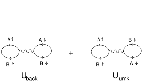
FIG. 11.: The effective coupling constant involved in the AFM response function.

These couplings are the renormalized couplings given by (20), (21). In the derivation of (24) we have substituted the value of ${\cal R}_{0}$ by its renormalized value ${\cal R}$.

At this stage it is worth to notice the difference of this procedure with a usual RPA computation. In view of fig. 10, we could be tempted to write down an integral equation for the complete response function of the type

$${\cal R}={\cal R}_{0}-U{\cal R}_{0}{\cal R}={\cal R}_{0}(1-U{\cal R})\;\;,$$

which can be summed up to give the RPA result. This procedure relies strongly upon the knowledge of the response function in the absence of interaction and on the assumption that the interacting quantities can be obtained adiabatically from the non–interacting ones. This is correct in the case of Fermi–liquid like systems where the single–particle properties of the full system are connected adiabatically with the vacuum of the free system. Such a procedure breaks down completely in the D=1 case where the interaction renormalizes strongly the single–particle properties. The Van Hove system that we are studying resembles the D=1 case in the respect that quasiparticles cease to make sense once we get too close to the Fermi line, i.e, when the cutoff is taken to zero. The particle–hole buble computed in this case does not make sense and can not be used as a starting point of a perturbative computation. What we do instead, similar to what is done in the D=1 case, is to rely upon the values of the naked response function for an energy close to the value of the cutoff $E_{c}$ where the Fermi–liquid behavior of the system can be assumed. We compute the scaling evolution of the response function upon integration of a strip of high–energy modes well above the Fermi line where the free Fermi propagator does make sense and obtain a differential equation for the response functions which can describe the physical properties of the system for energies below the critical frequencies where the couplings diverge.

The study of the ferromagnetic response function can be done following the same steps. It is given by the correlation of the uniform magnetization, $\rho_{\uparrow}(0,\omega)-\rho_{\downarrow}(0,\omega)$. The particle-hole bubble in this case has the prefactor $c=1/\sqrt{1-4(t^{\prime}/t)^{2}}$. The equation for $R_{FM}$ is

$$\frac{\partial R_{FM}}{\partial E_{c}}=-\frac{c}{\pi^{2}t}\frac{1}{E_{c}}+\frac{c}{2\pi^{2}t}\left(U_{intras}+U_{inters}\right)\frac{1}{E_{c}}R_{FM}\;\;\;.$$ (25)

It is easily seen that the operators related to charge-density-wave and s-wave superconducting instabilities do not develop divergent correlations at small $\omega$. The scaling equation for the response function ${\cal R}_{CDW}$ computed with the previous techniques is

$$\frac{\partial R_{CDW}}{\partial E_{c}}=-\frac{c^{\prime}}{\pi^{2}t}\frac{1}{E_{c}}-\frac{c^{\prime}}{2\pi^{2}t}\left(U_{back}+U_{umk}\right)\frac{1}{E_{c}}R_{CDW}\;\;\;,$$ (26)

and goes to zero as the couplings grow large. The same happens with ${\cal R}_{SCS}$.

The phase diagram in the $t^{\prime}-U$ plane is drawn by looking at the competition among ferromagnetic, antiferromagnetic and d-wave superconducting instabilities.

We recall that $U_{intras}+U_{inters}$ and $U_{back}+U_{umk}$ have the same flow, within the present model. Therefore, we may discern at once that whenever $c>c^{\prime}$ the ferromagnetic response function $R_{FM}$ prevails over $R_{AFM}$.

The study of the d–wave superconducting response function differs from the previous ones in various respects. First, as can be seen from the definition of ${\cal R}_{SCD}$, it is the second kind of diagrams in the first line of fig. 10 what contributes to the renormalization of the response function at first order in U. This implies that the effective coupling constant in this case has a relative minus sign being $U_{SCd}=U_{umk}-U_{intra}$. Next and more important, the dependence on the cutoff of the correlator $R^{0}_{SCD}$ given by the diagrams at strictly zero total momentum has a log squared singularity of the form $\log^{2}(E_{c}/\omega)$. We can still derive scaling equations in this case due to the fact that the dependence of the equation on the energy and the cutoff maintains the same same functional form what allows us to trade the cutoff by the energy.

The equation for $R_{SCd}$ reads then

$$\frac{\partial R_{SCd}}{\partial E_{c}}=-\frac{c}{2\pi^{2}t}\frac{\log(E_{c}/\omega)}{E_{c}}-\frac{c}{2\pi^{2}t}\left(U_{intra}-U_{umk}\right)\frac{\log(E_{c}/\omega)}{E_{c}}R_{SCd}$$ (27)

This equation also shows a homogeneous scaling of $R_{SCd}$ on $\omega/E_{c}$, like in the previous cases.

We shall interpret the previous equations in the sense that, for a given t’ and U, the system will be in a phase given by the response function that divergest first – or grows larger – at the largest frequency. The frequencies can be obtained by integrating the RG equations under the initial conditions that, at energies of the order of the cutoff, the response functions are finite. This gives us the following equations. In the region where $c>c^{\prime}$ where the ferromagnetic response function dominates, neglecting the constant term in (25), and taking the renormalized couplings as given by (20), (21), we have

$$\frac{\partial{\cal R}_{FM}}{\partial E_{c}}\sim\frac{c}{2\pi^{2}t}\;\;\left[\frac{U_{0}}{1+U_{0}\>c/(2\pi^{2}t)\>\log(\omega/E_{c})}\;+\;\frac{U_{0}}{1+U_{0}\>c^{\prime}/(2\pi^{2}t)\>\log(\omega/E_{c})}\right]\;\frac{1}{E_{c}}{\cal R}_{FM}\;\;,$$ (28)

whose integration gives

$${\cal R}_{FM}\sim{\cal R}_{0}\;\frac{1}{1+c/2\pi^{2}t\;U_{0}\log\omega/E_{c}}\left(\frac{1}{1+c^{\prime}/2\pi^{2}t\;U_{0}\log\omega/E_{c}}\right)^{c/c^{\prime}}\;\;.$$ (29)

The integration of the AFM response function following the same steps gives in the region $c^{\prime}>c$ :

$${\cal R}_{AFM}\sim{\cal R}_{0}\;\frac{1}{1+c^{\prime}/2\pi^{2}t\;U_{0}\log\omega/E_{c}}\left(\frac{1}{1+c/2\pi^{2}t\;U_{0}\log\omega/E_{c}}\right)^{c^{\prime}/c}\;\;.$$ (30)

The divergent flow of the superconducting response function is given by

$${\cal R}_{SCd}\sim{\cal R}_{0}\;\left(1+\frac{U_{0}c}{2\pi^{2}t}\log(\omega/E_{c})\right)^{2\pi^{2}t/U_{0}c}\frac{1}{\left(1+\frac{U_{0}t}{2\pi^{2}t}\log(\omega/E_{c})\right)^{2\pi^{2}t\frac{c}{c^{\prime 2}U_{0}}}}\;\;.$$ (31)

Putting the previous results all together, we arrive at the phase diagram shown in fig. 12.

FIG. 12.: Phase diagram in the (t’,U) plane. The dotted lines are contour lines corresponding to the critical frequencies shown in the figure.

From inspection of Eq. (27), it is clear that divergent correlations in the d-wave channel arise for $U_{intras}-U_{umk}<0$. According to the above results, this only happens for $c<c^{\prime}$, that is, outside the region of the phase diagram where $R_{FM}>R_{AFM}$. This confirms that a ferromagnetic regime sets in for values of $t^{\prime}$ above the critical value $t_{c}^{\prime}\approx 0.276t$ at which $c=c^{\prime}$. For values below $t_{c}^{\prime}$, there is a competition between $R_{AFM}$ and $R_{SCd}$, which requires the analysis of the respective behaviors close to the critical frequency at which the response functions diverge. As a general trend, the response function $R_{SCd}$ dominates over $R_{AFM}$ in the regime of weak interaction, the strength being measured with regard to both the bare coupling constant and the value of the $c^{\prime}$ parameter. The reason for such behavior is that at weak interaction strength the RG flow has a longer run to reach the critical frequency, and at small frequencies the logarithmic density of states in Eq. (27) makes $R_{SCd}$ to grow larger. The border where the crossover between the antiferromagnetic and the superconducting instability takes place is shown in the $t^{\prime}-U$ phase diagram of Fig. 10. At sufficiently large values of $U$ and small values of $t^{\prime}$, the leading instability of the system turns out to be antiferromagnetism. This is in agreement with weak coupling RG analyses applied to the Hubbard model[8, 9, 10]. Thus, there exists a region of the phase diagram where superconductivity is the leading instability. The critical frequencies at which the instability takes place are $\sim 10^{-2}E_{c}$. Taking values for $E_{c}$ of the order of the conduction bandwidth in the cuprates, $\sim 1$eV, and $U\sim E_{c}$, we obtain critical temperatures $\sim 100$K.

The physical mechanism that induces an electronic pairing out of purely repulsive interactions is the Kohn–Luttinger mechanism [29] according to which the competition between two different kinds of –repulsive– interactions, can modulate the net interaction at large frquencies giving rise to zones of attraction. This mechanism is known to take place in D=3 for the usual Coulomb interaction with spherical symmetry but there it becomes effective at very low temperatures and at very high values of the angular momentum. In two dimensions however and in a model like the one proposed here, due to the strong anisotropy of the Fermi line[36], the Kohn–Luttinger mechanism becomes much more efficient and can drive superconductivity at frequencies accesible experimentally.

V Conclusions and open problems

We start this section by mentioning the differences and similarities between the present work and related works in the literature. Concerning the papers that apply RG techniques, we must establish a difference between those appearing before and after the modern approach reviewed in [11]. In particular scaling methods were used in [8, 10] where they treat the whole Fermi surface trying to arrive to a low–energy effective action. What we do follows the approach described in [12]. We postulate a low–energy effective action valid only in the proximity of the Fermi line, and study its stability under renormalization. The same approach in the case of Fermi–liquid systems yields surprisingly good results because the postulated action turns out to be the attractive fixed point in all cases –in the absence of BCS instability– . In the present case it is somehow unfortunate that the effective action is unstable in the sense that all the interactions are marginally relevant and we do not see a fixed point where it flows to. This situation is very similar to what happens in systems of coupled one–dimensional chains [40] where any inter–chain coupling changes drastically the behavior of a single chain. From our point of view, this behavior does not invalidate the study presented in this paper as we believe that the action (4) will govern the behavior of any system of the type discussed when the filling lies close to the Van Hove singularities.

Concerning our previous work [16, 17] the main difference with the present work is that we have studied before spin–independent extended interactions –of the type $V(r)$ described in the introduction – and put the emphasis in the possibility of getting a pairing instability of electronic origin. In these cases we obtained an attractive fixed point at the origin. The present work introduces the spin dependence and deals with strictly local interactions what allows us to obtain the rich phase diagram of fig. 12. It is the spin dependence of the interactions what renders the action unstable to all interactions.

As a summary of the results, we have shown that the purely repulsive Hubbard t–t’ model at the Van Hove singularity exhibits a variety of instabilities at low energy or temperature. In particular, we have seen that it supports a superconducting instability with d–wave symmetry coexisting in the same region of parameter space with an antiferromagneting instability. This feature has been recently found in [33] by means of a mean–field computation. There is nowdays a general agreement on the fact that d–wave superconductivity is the strongest experimental sign in hole doped cuprates.

We remark that this result is obtained within a RG approach that provides a rigorous computational framework, with no other assumption than the weakness of the bare interaction. The instabilities are led by an unstable RG flow, and the singular behavior of the response functions has been given a more solid foundation than the standard RPA computations. On the other hand, the renormalized interactions remain during most part of the flow in the weak coupling regime for $U<t$.

From a formal point of view, the second relevant conclusion within our RG approach is the existence of a ferromagnetic regime in the $t-t^{\prime}$ model, above a certain value of the $t^{\prime}$ parameter. This is consistent with the results obtained in [34] close to $t^{\prime}=0.5t$. Though our results refer to the weak coupling regime, they show that antiferromagnetic, ferromagnetic and superconducting phases are all realized in the $t-t^{\prime}$ Hubbard model. The superconducting instability has greater strength at the boundary with the antiferromagnetic instability, as it also happens in other approaches to high-$T_{c}$ superconductivity[35].

In our case, the diagrams responsible for the apppearance of superconductivity cannot be interpreted in terms of the exchange of antiferromagnetic fluctuations, as in the works mentioned earlier[35]. Those diagrams which contain bubbles mediating an effective interaction between electron propagators are cancelled, to all orders, by vertex corrections (see Fig. 3). Superconductivity arises from the type of diagrams first studied by Kohn and Luttinger[29]. The strong anisotropy of the Fermi surface greatly enhances the Kohn-Luttinger mechanism, with respect to its effect in an isotropic metal[16, 17, 36].

The wide range for superconductivity is consistent with the results from quantum Monte Carlo computations[37], as well as with results obtained by exact diagonalization of small clusters in the strong coupling regime[38].

Our results support the idea that d-wave superconductivity and antiferromagnetism arise from the same type of interactions. Antiferromagnetism, however, does not favor the existence of superconductivity, but competes with it in the same region of parameter space. The renormalization group analysis done in the present work does not allow to study the possible existence of a quantum critical point at the end of the line separating the antiferromagnetic and the superconducting phases where a phase of higher symmetry has been postulated [39]. Similar physical processes seem to be responsible for the appearance of anisotropic superconductivity in systems of coupled repulsive 1D chains[40]. The Fermi surface of a single chain is unable to give rise to this type of superconductivity. A soon as this limitation is lifted, superconductivity occupies a large fraction of the phase diagram previously dominated by antiferromagnetic fluctuations.

We now report on the open problems left in this work.

As a technical remark, we have neglected self-energy corrections in the confidence based on previous computations [17] that they will not change drastically the Fermi-Liquid form. Our propagators are fermion propagators as we expect the elementary excitations of the system to have a fermionic character. Here comes the subtle point of the nature of the free fixed point being an isolated point in the coupling constant phase space (fig. 8). Unlike what happens in one dimensional systems where the quasiparticle pole is destroyed by the interaction, our interpretation of fig. 8 is that the Van Hove model has to be considered as an effective model whose validity starts when the Fermi surface of an otherwise Fermi liquid, sits close to the Van Hove singularity. Such a system will never show a Fermi liquid character as the instabilities described in the paper will take over. This is confirmed by the experimental results. For overdoped samples, the Fermi surface is closed and electron-like. In a non–interacting model, the Fermi surface would grow as more electrons are added until it would reached the Van Hove points, acquiring a shape shown in fig. 1. What is observed instead is that as more electrons are added, the system develops a gap near the Van Hove points [30].

The results reported in this work can be extended to fillings away from the van Hove singlarity, provided that the distance of the chemical potential to the singularity is smaller than the energy scale at which the instability takes place. The chemical potential tends to be pinned to the singularity because of the non trivial RG flow of the chemical potential itself[16, 17]. Hence, these calculations can be applied to a finite range of fillings around that appropiate to the singularity.

Acknowledgments One of us (MAHV) thanks the Institute of Advanced Study of Princeton for its hospitality during the summer of 1997 when the manuscript was completed.

REFERENCES

- [1] J. G. Bednorz and K. A. Muller, Z. Phys. B 64 (1986) 189.
- [2] A very good summary of the main theoretical ideas is contained in the various reports of High Temperature Superconductivity, proceedings of 1989 Los Alamos Symposium, K. S. Bedell, D. Coffey, D. E. Meltzner, D. Pines, J. R. Schrieffer eds., Addison-Wesley 1990.
- [3] E. M. Lifshitz and L. P. Pitaevskii, Statistical Physics, Part 2 (Pergamon Press, Oxford, 1980).
- [4] P. W. Anderson, Science 235 (1987) 1196. For a complete account of Anderson’s model, see The theory of superconductivity in the high-Tc cuprates, Princeton University Press, 1997.
- [5] F. C. Zhang and T. M. Rice, Phys. Rev. B 37 (1988) 3759.
- [6] Proceedings of the Nato Advanced Workshop on The physics and mathematical physics of the Hubbard model, Campbell et al. eds., Plenum Press 1995.
- [7] P. A. Lee and N. Read, Phys. Rev. Lett. 58 (1988) 2691.
- [8] H. J. Schulz, Europhys. Lett. 4 (1987) 51.
- [9] J. E. Dzyaloshinskii, Pis’ma Zh. Eksp. Teor. Fiz. 46 (1987) 97 [JETP Lett. 46, 118 (1987)].
- [10] D. Zanchi and H. J. Schulz, Phys. Rev. B 54 (1996) 9509.
- [11] R. Shankar, Rev. Mod. Phys. 66 (1994) 129.
- [12] J. Polchinski, in Proceedings of the 1992 TASI in Elementary Particle Physics, J. Harvey and J. Polchinski eds. (World Scientific, Singapore, 1992).
- [13] J. Labbé and J. Bok, Europhys. Lett. 3 (1987) 1225. J. Friedel, J. Phys. (Paris) 48 (1987) 1787; 49 (1988) 1435.
- [14] R. S. Markiewicz, J. Phys. Condens. Matter 2 (1990) 665. R. S. Markiewicz and B. G. Giessen, Physica (Amsterdam) 160C (1989) 497. A complete review of the Van Hove model with references is A survey of the Van Hove scenario for high-Tc superconductivity with special emphasis on pseudogaps and stripped phases, cond-mat/9611238, to be published in J. Phys. Chem. Sol.
- [15] C. C. Tsuei et al., Phys. Rev. Lett. 65 (1990) 2724; P. C. Pattnaik et al., Phys. Rev. B 45 (1992) 5714.
- [16] J. González, F. Guinea and M. A. H. Vozmediano, Europhys. Lett. 34 (1996) 711.
- [17] J. González, F. Guinea and M. A. H. Vozmediano, Nucl. Phys. B 485 (1997) 694.
- [18] L. B. Ioffe and A. J. Millis, Phys. Rev. B 54 (1996) 3645.
- [19] Z.-X. Shen et al., Science 267 (1995) 343, and references therein.
- [20] K. Gofron et al., Phys. Rev. Lett. 73, (1994) 3302.
- [21] J. Sólyom, Adv. Phys. 28 (1979) 201. V. J. Emery, in Highly Conducting One-Dimensional Solids, edited by J. T. Devreese, R. P. Evrard and V. E. Van Doren (Plenum, New York, 1979). H. J. Schulz, “Interacting fermions in one dimension”, cond-mat/9302006 (1993).
- [22] G. Litak et al., preprint cond-mat/9801035.
- [23] J. V. Alvarez, J. González, F. Guinea and M. A. H. Vozmediano, preprint cond-mat/9705165 (1997), to appear in the J. Phys. Soc. Jpn.
- [24] Sir Nevill Mott, Metal-Insulator Transitions, Taylor and Francis, London 1974.
- [25] H. Q. Lin and J. E. Hirsch, Phys. Rev. B 35, 3359 (1987).
- [26] P. Bénard, L. Chen and A. M. Tremblay, Phys. Rev. B 47 (1993) 15 217; Q. Si, T. Zha, K. Levin and J. P. Lu, ibid. 47 (1993) 9055; A. Nazarenko et al., ibid. 51 (1995) 8676; D. Duffy and A. Moreo, ibid. 52 (1995) 15607; A. F. Veilleux et al., ibid. 52 (1995) 16255.
- [27] J. González, M. A. Martín-Delgado, G. Sierra and M. A. H. Vozmediano, Quantum Electron Liquids and High- Superconductivity (Springer-Verlag, Berlin, 1995).
- [28] D. J. Amit, Field Theory, Renormalization Group and Critical Phenomena, Chap. 8 (McGraw-Hill, New York, 1978).
- [29] W. Kohn and J. M. Luttinger, Phys. Rev. Lett. 15 (1965) 524.
- [30] D. M. King, D. S. Dessau, A. G. Loesser, Z. -X. Shen, and B. O. Wells, J. Phys. Chem. Solids 56 (1996) 1865.
- [31] J. V. Alvarez, J. González, F. Guinea and M. A. H. Vozmediano, in preparation.
- [32] C. M. Varma et al., Phys. Rev. Lett. 63, 1996 (1989).
- [33] M. Murakami and H. Fukuyama, cond-mat/9710113 (1997).
- [34] S. Sorella, R. Hlubina and F. Guinea, Phys. Rev. Lett. 78 (1997) 1343.
- [35] N. E. Bickers, D. J. Scalapino and S. R. White, Phys. Rev. Lett. 62, 961 (1989); E. Dagotto, J. Riera and A. P. Young, Phys. Rev. B 42, 2347 (1990); P. Monthoux and D. Pines, Phys. Rev. Lett 69, 961 (1992); E. Dagotto and J. Riera, ibid. 70, 682 (1993); E. Dagotto, A. Nazarenko and A. Moreo, ibid. 74, 310 (1995). K. Maki and H. Won, Phys. Rev. Lett. 72, 1758 (1994).
- [36] J. González, F. Guinea and M. A. H. Vozmediano, Phys. Rev Lett. 79 (1997) 3514.
- [37] T. Husslein et al., Phys. Rev. B 54, 16179 (1996).
- [38] J. González and J. V. Alvarez, Phys. Rev. B 56 (1997) 367.
- [39] S. Zhang, Science 275 (1997) 1089.
- [40] H.-H. Lin, L. Balents and M. P. A. Fisher, preprint (cond-mat/9703055).