[

Profile scaling in decay of nanostructures

Abstract

The flattening of a crystal cone below its roughening transition is studied by means of a step flow model. Numerical and analytical analyses show that the height profile, $h(r,t)$, obeys the scaling scenario $\partial h/\partial r={\cal F}(rt^{-1/4})$. The scaling function is flat at radii $r<R(t)\sim t^{1/4}$. We find a one parameter family of solutions for the scaling function, and propose a selection criterion for the unique solution the system reaches.

]

In recent years it has become technologically possible to design and manufacture crystalline nanostructures, which are of tremendous importance for the fabrication of electronic devices. In many cases, these nanostructures are thermodynamically unstable, and tend to decay with time. This phenomenon has triggered experimental and theoretical efforts to try and understand the decay process[3, 4, 5, 6, 7, 8, 9, 10, 11, 12, 13, 14, 15]. Under fairly robust conditions, the decay of a nanostructure at low temperatures (below the roughening temperature, $T_{R}$) is dominated by the motion of atomic steps on the surface. Hence, attempts have been made to understand and predict the relaxation dynamics of simple step configurations.

In this work we analyze, numerically as well as analytically, the time evolution of a crystalline cone formed out of circular concentric steps. The decay of other types of nanostructures such as bi-periodic surface modulations has been studied experimentally on Si(001) by Tanaka et al. [3]. Rettori and Villain[4] studied this problem theoretically in the case of small amplitude modulations. Our study, on the other hand, is relevant to large amplitude modulations and in this sense is complimentary to their work. We find that the height of the cone decays with time as $h(0)-h(t)\sim t^{1/4}$ and the radius of the plateau at the top of the cone grows with time as $R(t)\sim t^{1/4}$.

Consider the surface of an infinite crystalline cone, made out of circular concentric steps of radii $r_{i}(t)$, separated by flat terraces. The step index $i$ grows in the direction away from the center of the cone. We assume no deposition of any new material, no evaporation and no transport of atoms through the bulk. To calculate the time dependence of the radii, we have to solve the diffusion equation for adatoms on the terraces with boundary conditions at the step edges, taking into account the repulsive interactions (of the form $G(r_{i+1}-r_{i})^{-2}$) between steps. Using a standard approach to do this [4, 16], we arrived at a set of equations of motion for the step radii. It is convenient to present these equations in terms of dimensionless radii, $\rho_{i}$, and dimensionless time $\tau$:

$$\rho_{i} = \frac{T}{\Omega\Gamma}\cdot r_{i}\;,$$

$$\tau = D_{s}C^{0}_{eq}\Omega\cdot\left(\frac{T}{\Omega\Gamma}\right)^{2}\cdot\left(1+\frac{D_{s}T}{k\Omega\Gamma}\right)\cdot t\;.$$

$C^{0}_{eq}$ is the equilibrium concentration of a straight isolated step, $T$ is the temperature, $\Gamma$ is the step line tension, $\Omega$ is the atomic area of the solid and $D_{s}$ is the diffusion constant of adatoms on the terraces. $k$ is a kinetic coefficient associated with attachment and detachment of adatoms to and from steps.

The equations of motion in terms of these variables take the form

$$\dot{\rho}_{i} \equiv \frac{d\rho_{i}}{d\tau}=\frac{a_{i}-a_{i-1}}{\rho_{i}}\;,\;\;\mbox{with}$$ (1)

$$a_{i} = \frac{\frac{1}{\rho_{i}}-\frac{1}{\rho_{i+1}}+2g\left(\xi_{i}-\frac{\rho_{i-1}}{\rho_{i}+\rho_{i-1}}\xi_{i-1}-\frac{\rho_{i+2}}{\rho_{i+2}+\rho_{i+1}}\xi_{i+1}\right)}{\left(1-q\right)\ln\frac{\rho_{i}}{\rho_{i+1}}-q\left(\frac{1}{\rho_{i}}+\frac{1}{\rho_{i+1}}\right)}$$ (2)

$$\xi_{i} = \left(\rho_{i+1}-\rho_{i}\right)^{-3}\;,$$ (3)

where the velocities of the first and second steps are modified to include interactions only with existing steps. Eq. (1) depends on two parameters: $g$ and $q$. $g=\frac{T^{2}G}{\Omega^{2}\Gamma^{3}}$ measures the strength of step-step interactions $G$ relative to the line tension $\Gamma$, while the parameter $q=(1+\frac{k\Omega\Gamma}{D_{s}T})^{-1}$ specifies the rate limiting process in the system. When $D_{s}\gg k$ (or $q\rightarrow 1$), diffusion across terraces is fast and the rate limiting process is attachment and detachment of adatoms to and from steps. When $D_{s}\ll k$ (or $q\rightarrow 0$), the steps act as perfect sinks and the rate limiting process is diffusion across terraces.

We integrated Eqs. (1) numerically both in the diffusion limited (DL) and in the attachment/detachment limited (ADL) cases. When the repulsive interactions between steps are weak (i.e. $g$ is small), there is a striking difference between the dynamics in the two limits. In the ADL case the system becomes unstable towards step bunching, whereas in the DL case there is no such instability. However, when $g$ is large enough the instability disappears even in the ADL case. We limit our discussion to situations where the step bunching instability does not occur. Fig. 1 shows the time evolution of initially uniformly spaced steps with unit step separation in the ADL case.

      

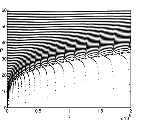
FIG. 1.: Time evolution of the step radii in the ADL case with $g=0.01$. The front can be fitted by a $\tau^{1/4}$ power law (dashed line).

Each line in the figure describes the radius of one step as a function of time. We note that the innermost step shrinks while the other steps expand by absorbing the atoms emitted by the first step. When the innermost step disappears, the next step starts shrinking and so on. The disappearance time of the $n^{th}$ step, $\tau_{n}$, grows with $n$ as $\tau_{n}\sim n^{4}$. This process results in a propagating front which leaves a growing plateau behind it. At large times, the (dimensionless) position of this front behaves as $\rho_{{\mbox{\rm}front}}(\tau)\sim\tau^{1/4}$. A similar picture arises in the DL case with differences in the details of the individual step trajectories. This power law is an indication of a much more general and interesting phenomenon. It turns out that for large times, not only the front position but also the positions of minimal and maximal step densities scale as $\tau^{1/4}$. In fact, the step density $D(\rho,\tau)$ obeys the following scaling scenario: There exist scaling exponents $\alpha$, $\beta$ and $\gamma$ which define the scaled variables $x\equiv\rho\tau^{-\beta/\gamma}$ and $\theta\equiv\tau^{1/\gamma}$. In terms of these variables $D(\rho,\tau)=\theta^{\alpha}F(x,\theta)$, where the scaling function $F$ is a periodic function of $\theta$ with some period $\theta_{0}$. Our ansatz is somewhat weaker than standard scaling hypotheses, which would assume $F$ is independent of $\theta$. The necessity to introduce a periodic dependence of $F$ on $\theta$ is a manifestation of the discrete nature of the steps. Thus the disappearance time of step $n$ is $\tau_{n}=(n\theta_{0})^{\gamma}$. An immediate consequence of the scaling ansatz is that if we define $\theta=\bar{\theta}+n\theta_{0}$ with $0\leq\bar{\theta}<\theta_{0}$, and plot $\theta^{-\alpha}D\left(x\theta^{\beta},\theta^{\gamma}\right)$ against $x$, all the data with different values of $n$ and the same value of $\bar{\theta}$ collapse onto a single curve.

To verify that our system obeys this scaling ansatz, we define the step density at a discrete set of points in the middle of the terraces:

$$D\left(\frac{\rho_{i}(\tau)+\rho_{i+1}(\tau)}{2},\tau\right)=\frac{1}{\rho_{i+1}(\tau)-\rho_{i}(\tau)}\;.$$ (4)

Fig. 2 is a plot of $D(\rho,\tau)$ as a function of $x=\rho\tau^{-1/4}$ for a fixed value of $\bar{\theta}$ and 12 different values of $n$ in the ADL case. The excellent data collapse shows that our scaling ansatz indeed holds with $\alpha=0$, $\beta=1$ and $\gamma=4$. Data collapse of similar quality is achieved in the DL case with the same values of the exponents. The dependence of the scaling function on $\theta$ is very weak in the DL case, and is more pronounced in the ADL case.

      

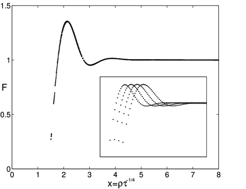
FIG. 2.: Data collapse of the density function in the ADL case with $g=0.01$. The values of the scaling exponents used here are $\alpha=0$, $\beta=1$ and $\gamma=4$. This figure shows density functions with 12 different values of $n$ and the same value of $\bar{\theta}$, as a function of $x=\rho\tau^{-1/4}$. Some of the unscaled data are shown in the inset.

The above results suggest that the time evolution of the system can be described by a density, which is a continuous function of both position and time. In the remainder of this paper we will derive such a continuum model, carry out a scaling analysis to evaluate the scaling exponents analytically, and calculate the scaling function.

Motivated by the simulation results we assume that the scaling ansatz holds. This is already sufficient to calculate the values of $\alpha$ and $\beta$. First, we derive a relation between these scaling exponents by considering the height profile $h(\rho,\tau)$. Assuming steps of unit height, the profile is related to the step density by

$$h(\rho,\tau)=h_{0}(\tau)-\int_{0}^{\rho}D(\rho^{\prime},\tau)d\rho^{\prime}\;,$$ (5)

where $h_{0}(\tau)$ is the height at the origin. Far enough (when $\rho\rightarrow\infty$), $h(\rho,\tau)$ does not change with time, i.e. $\lim_{\rho\rightarrow\infty}(h(\rho,\tau)-h(\rho,0))=0$. Combining this with Eq. (5), we arrive at the expression

$$h_{0}(0)-h_{0}(\tau)=\tau^{\frac{\alpha+\beta}{\gamma}}\int_{0}^{\infty}(F(\infty,0)-F(x,\theta))dx\;,$$ (6)

where we have used the definition of the function $F$. On the other hand, $h_{0}(0)-h_{0}(\tau_{n})=n$ because $\tau_{n}$ is the disappearance time of the $n^{th}$ step. $\gamma$ satisfies the relation $\tau_{n}\sim n^{\gamma}$, and therefore we have $h_{0}(0)-h_{0}(\tau_{n})\sim\tau_{n}^{1/\gamma}$. This and the $\tau^{(\alpha+\beta)/\gamma}$ dependence in Eq. (6) lead to the relation $\alpha+\beta=1$.

In addition, conservation of the total volume of the system implies that $\int_{0}^{\infty}\rho h(\rho,\tau)d\rho$ is independent of $\tau$. Integration by parts of the derivative of this integral with respect to $\tau$ yields the following equation:

$$\int_{0}^{\infty}\rho^{2}\frac{\partial D(\rho,\tau)}{\partial\tau}d\rho=0\;.$$ (7)

Evaluation of this integral in terms of the function $F$ and the scaled variables $x$ and $\theta$ shows the integral diverges unless $\alpha=0$ [17]. Combining this with $\alpha+\beta=1$, we conclude that $\beta=1$.

To evaluate the scaling exponent $\gamma$ and the scaling function $F$, we continue with the equation for the full time derivative of the step density $D$:

$$\frac{dD}{d\tau}=\frac{\partial D}{\partial\tau}+\frac{\partial D}{\partial\rho}\cdot\frac{d\rho}{d\tau}\;.$$ (8)

Eq. (8) can be evaluated in the middle of the terrace between two steps (i.e. at $\rho=(\rho_{i}(\tau)+\rho_{i+1}(\tau))/2$). The l.h.s. of (8) is calculated by taking the time derivative of Eq. (4): $dD/d\tau=-D^{2}(\dot{\rho}_{i+1}-\dot{\rho}_{i})$. This together with the fact that $d\rho/d\tau=((\dot{\rho}_{i}(\tau)+\dot{\rho}_{i+1}(\tau))/2$ leads to the relation

$$\frac{\partial D}{\partial\rho}\frac{\dot{\rho}_{i+1}+\dot{\rho}_{i}}{2}+\frac{\partial D}{\partial\tau}+D^{2}(\dot{\rho}_{i+1}-\dot{\rho}_{i})=0\;,$$ (9)

where the step velocities $\dot{\rho}_{i}$ can be expressed in terms of the $\rho_{i}$’s using Eq. (1).

Now we change variables to $\theta$ and $x_{i}\equiv\rho_{i}\theta^{-1}$, and transform Eq. (9) into an equation for the scaling function $F$. In terms of these variables, Eq. (4) takes the form

$$x_{i+1}-x_{i}=\frac{\theta^{-1}}{F\left((x_{i+1}+x_{i})/2,\theta\right)}\;.$$ (10)

According to this, the difference between successive $x_{i}$’s is of order $\theta^{-1}$ wherever $F$ does not vanish. In the large $\theta$ (long time) limit these differences become vanishingly small. This allows us to go to a continuum limit in the variable $x$, by expanding all the terms in the equation for the scaling function $F$ in the small parameter $\theta^{-1}$. The final result of these manipulations is the following differential equation for $F$:

$$-F^{\prime}\cdot\frac{x}{\gamma} + \theta^{\gamma-4}\left(F^{\prime}\cdot\frac{A}{2}+F^{2}B\right)$$ (11)

$$+\frac{\theta}{\gamma}\cdot\frac{\partial F}{\partial\theta} + O(\theta^{\gamma-5})=0\;.$$ (12)

$A$ and $B$ are known expressions involving $F$,$F^{\prime}$,$F^{\prime\prime}$,$F^{\prime\prime\prime}$, $F^{\prime\prime\prime\prime}$, where the primes denote partial derivatives with respect to $x$. The existence of derivatives up to fourth order in this equation is a consequence of the fact that each step “interacts” with four other steps (two on each side) through the equations of motion (1). A detailed derivation of the continuum model and the exact expressions for $A$ and $B$ will be given elsewhere [17].

Consider Eq. (12) at large $\theta$. Our expansion in the small parameter $\theta^{-1}$ is valid only at values of $x$ where $F$ does not diverge or vanish (see above). Therefore, the first term in Eq. (12) is $O(1)$. This term has to be canceled by the second term if we require $F$ to satisfy a single differential equation. Hence, we must have

$$\gamma=4\;.$$ (13)

The fourth term vanishes as $\theta\rightarrow\infty$, since $\gamma-5<0$ and the third term must vanish as well. Therefore, in the large $\theta$ limit, $F$ is only a function of $x$, and we are left with an ordinary differential equation for $F$:

$$F^{\prime}\left(\frac{A}{2}-\frac{x}{4}\right)+F^{2}B=0\;.$$ (14)

Let us emphasize that our continuum model is valid for arbitrarily large surface curvature and slope (unlike other treatments [4, 8]). Moreover, since our model is an expansion in the truly small parameter $\theta^{-1}$ (see Eq. (10)) it becomes exact in the large $\theta$ (long time) limit. Note that in going to the continuum limit we lost the periodic dependence of $F$ on $\theta$, which is a manifestation of the discrete nature of the steps.

We now turn to study the solutions of Eq. (14). We will consider only the DL case, but an equivalent treatment can be applied to more general situations [17]. In the DL case Eq. (14) becomes [12]

$$g\left(12F^{\prime}F^{\prime\prime\prime}+3FF^{\prime\prime\prime\prime}+9F^{\prime\prime 2}+\frac{15F^{\prime}F^{\prime\prime}+5FF^{\prime\prime\prime}}{x}\right.$$ (16)

$$\left.-\frac{7\left(F^{\prime 2}+FF^{\prime\prime}\right)}{x^{2}}+\frac{6FF^{\prime}}{x^{3}}-\frac{3F^{2}}{x^{4}}\right)-\frac{xF^{\prime}}{4}-\frac{3}{x^{4}}=0\;.$$

Without loss of generality, we choose the boundary condition at infinity to be $F(\infty)=1$. Any other choice is equivalent to our choice with a different value of the interaction parameter $g$, since Eq. (16) is invariant under the transformation $F\rightarrow aF$, $x\rightarrow a^{-1/4}x$ and $g\rightarrow a^{-2}g$. Numerical solutions of Eq. (16) which satisfy $F(\infty)=1$ indicate that there exists a point $x=x_{0}$ near which $F$ behaves as $F(x)\sim\sqrt{x-x_{0}}$. An analytical expansion of Eq. (16) for small $F$ also leads to the same conclusion. Thus, our model naturally predicts a singular point in the profile at which $F\rightarrow 0$. We can prove [17] that $x_{0}$ is the scaled position of the boundary of the plateau at the top of the hill.

In the derivation of Eq. (16) we assumed $F(x)\neq 0$. This is clearly violated on the plateau. Eq. (16) is therefore valid only at $x>x_{0}$, while for $x<x_{0}$, the solution for $F$ is simply $F=0$. Now we have to solve Eq. (16) for $x>x_{0}$ with some boundary conditions at $x=x_{0}$ together with the condition $F(\infty)=1$. In addition, we have to make sure that all the atoms expelled by the growing plateau at $x<x_{0}$ are absorbed by the steps at $x>x_{0}$. This is taken care of by the conservation law (7). We rewrite (7) in terms of scaled variables and get the following equation:

$\displaystyle\int_{0}^{\infty}x^{2}\left(F(x)-1\right)dx=\int_{x_{0}}^{\infty}x^{2}\left(F(x)-1\right)dx-\frac{x_{0}^{3}}{3}=0\;.$

To carry out the last integral we integrate Eq. (16) multiplied by $x^{2}$ from $x_{0}$ to $\infty$, and obtain the boundary condition

$$\lim_{x\rightarrow x_{0}}\left\{\vphantom{\frac{3}{x}}g\left(6FF^{\prime}+xFF^{\prime\prime}+xF^{\prime 2}\right.\right.$$ (18)

$$\;\;\;\;\;\;\;\;\left.\left.-3x^{2}FF^{\prime\prime\prime}-9x^{2}F^{\prime}F^{\prime\prime}\right)-\frac{3}{x}\right\}=0\;.$$

      

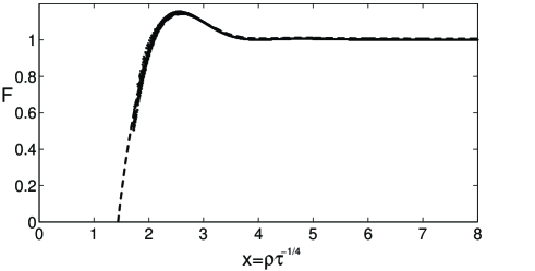
FIG. 3.: Data collapse of the density function in the diffusion limited case with $g=0.01$. Simulation data from several collapse periods are shown as dots, while the dashed line is the $x_{0}=x_{0}^{*}$ solution of Eq. (16).

So far, we have not determined the value of $x_{0}$. In fact, we solved Eq. (16) numerically and found a family of solutions satisfying the boundary conditions, which differ in the value of $x_{0}$. For $x_{0}<x_{0}^{*}\approx 1.44$ the equation does not have a solution. However, for any value of $x_{0}\geq x_{0}^{*}$ there is a single solution that satisfies the boundary conditions. Despite the existence of many solutions, our simulations indicate that the system reaches a unique scaling solution independent of initial conditions. Fig. 3 shows an impressive agreement between the $x_{0}=x_{0}^{*}$ solution and the data collapse of density functions taken from the simulations in the DL case. Thus, the system dynamically selects the scaling state with the minimal value of $x_{0}$. The precise nature of this selection mechanism is not yet understood and will be investigated in the future.

In summary, we have presented a complete description of the relaxation process of an infinite crystalline cone below it’s roughening transition. The hypothesis that in the long time limit the step density exhibits scaling leads to an accurate continuous model for the morphological evolution of the crystal. Using the model, we were able to derive the exact scaling exponents and the differential equation that describes the scaling function. This equation admits many solutions, and the system dynamically selects the one with the smallest plateau. We hope this work will motivate new experiments in which our predictions will be tested.

This research was supported by grant No. 95-00268 from the United States-Israel Binational Science Foundation (BSF), Jerusalem, Israel. D. Kandel is the incumbent of the Ruth Epstein Recu Career Development Chair.

REFERENCES

- [1] E-mail: israeli@wicc.weizmann.ac.il
- [2] E-mail: fekandel@wicc.weizmann.ac.il
- [3] S. Tanaka, N. C. Bartelt, C. C. Umbach, R. M. Tromp and J. M. Blakely, Phys. Rev. Lett. 78, 3342 (1997).
- [4] A. Rettori and J. Villain, J. Phys. France 49, 257 (1988).
- [5] K. Yamashita, H. P. Bonzel and H. Ibach, Appl. Phys. 25, 231 (1981); H. P. Bonzel and E. Preuss, Appl. Phys. A 35, 1 (1984); H. P. Bonzel and W. w. Mullins, Surf. Sci. 350, 285 (1996).
- [6] J. Villain, Europhys. Lett. 2, 531 (1986).
- [7] M. Uwaha, J. Phys. Soc. Jpn. 57, 1681 (1988).
- [8] M. Ozdemir and A. Zangwill, Phys. Rev. B 42, 5013 (1990).
- [9] F. Lancon and J. Villain, Phys. Rev. Lett. 64, 293 (1990).
- [10] C. C. Umbach, M. E. Keeffe and J. M. Blakely, J. Vac. Sci. Technol. A 9, 1014 (1991).
- [11] M. A. Dubson and G. Jeffers, Phys. Rev. B 49, 8347 (1994).
- [12] J. Hager and H. Spohn, Surf. Sci. 324, 365 (1995). The straight steps limit of our DL case coincides with the continuum theory of these authors.
- [13] M. V. Ramana Murty and B. H. Cooper, Phys. Rev. B 54, 10377 (1996). These Monte Carlo simulations agree with [4, 8].
- [14] E. S. Fu, M. D. Johnson, D. J. Liu, J. D. Weeks amd E. D. Williams, Phys. Rev. Lett. 77, 1091 (1996).
- [15] W. W. Mullins, J. Appl. Phys. 28, 333 (1957); 30, 77 (1959).
- [16] G. S. Bales and A. Zangwill, Phys. Rev. B 41, 5500 (1990).
- [17] N. Israeli and D. Kandel, unpublished.