A New Look at Low–Temperature Anomalies in Glasses

Abstract

We review a model–based rather than phenomenological approach to low–temperature anomalies in glasses. Specifically, we present a solvable model inspired by spin–glass theory that exhibits both, a glassy low–temperature phase, and a collection of double– and single–well configurations in its potential energy landscape. The distribution of parameters characterizing the local potential energy configurations can be computed, and is found to differ from those assumed in the standard tunneling model and its variants. Still, low temperature anomalies characteristic of amorphous materials are reproduced. More importantly perhaps, we obtain a clue to the universality issue. That is, we are able to distinguish between properties which can be expected to be universal and those which cannot. Our theory also predicts the existence, under suitable circumstances of amorphous phases without low–energy tunneling excitations.

1 Introduction

Ever since the first measurements of Zeller and Pohl [1] revealed that the specific heat and and the thermal conductivity of glassy systems at low temperatures are strikingly different from those of crystalline substances, the low temperature physics of glassy and amorphous materials has been a subject of intense research efforts, both experimentally and theoretically.

Specifically, it was found [1] that below approximately 1 K the specific heat of glassy materials scales approximately linearly with temperature, $C\sim T$ while the corresponding scaling for the thermal conductivity $\kappa$ is approximatly quadratic $\kappa\sim T^{2}$. Both findings contrast the $T^{3}$ behaviour of these quantities in crystals. Between 1  K and approximately 20 K the thermal conductivity exhibits a plateau and, then continues to rise as the teperature is further increased. The specific heat, too, changes its behaviour in the 1–20 K regime. It exhibits a bump if displayed in $C/T^{3}$ plots.

Particularly intriguing is the fact that the anomalous behaviour below 1 K appears to be universal in the sense that it is shared by virtually all glassy and amorphous materials, whereas the behaviour between 1 and 20 K seems to display a greater material dependence. The universality in the thermal conductivity data actually appears to go beyond the level of exponents, in that by a suitable rescaling with a constant depending on the Debeye temperature and the the sound velocity, thermal conductivity data for various substances can be scaled onto one master–curve both below and above, though not on the plateau [2].

It should be added that there is also an extensive body of experimental data characterizing the anomalous response of glassy and amorphous materials to external probes such as ultrasound or electromagnetic fields. The reader is invited to consult the reviews of Hunklinger et al. [5] or Phillips [6] on these matters.

The unusual material properties at low temperatures are usually attributed to the existence of a broad range of localized low–energy excitations in amorphous systems — excitations not available in crystalline materials. At energies below 1 K, these are believed to be tunneling excitations of single particles or (small) groups of particles in double–well configurations of the potential energy (DWPs). This is the main ingredient of the phenomenological so–called standard tunneling model (STM), independently proposed by Phillips [3] and by Anderson et al. [4]. As a second ingredient of the STM, it is supposed that the local DWPs in amorphous systems are random, and specific assumptions concerning the distribution of the parameters characterising them must be advanced (see below) to describe the experimental data below 1 K [3, 4].

Neither Phillips [3] nor Anderson et al. [4] consider excitations other than the tunneling excitation in the DWP structures postulated by them — their local degrees of freedom are thus true two–level systems (TLSs). As a consequence their model is unable to account for the different physics that appears in the temperature range between 1 and 20 K. However, different sets of low energy excitations in amorphous systems can exist: (i) Higher excitations in the abovementioned DWPs — a possibility that is surely contained in the physical picture advanced by Phillips or Anderson et al., but was justly considered irrelevant for the very low temperature regime and then somehow not reconsidered when problems with the model arose at temperatures above 1 K. (ii) Localized vibrations (localized phonons) in soft anharmonic single well configurations of the potential energy. The latter have been postulated (in addition to tunneling excitations in DWPs) within the, likewise phenomenological soft–potential model (SPM) [7, 8] to describe the physics above 1 K. Again, local potential energy configurations are supposed to be random, and specific assumptions concerning the distributions of the parameters characterizing them are required to account for the experimental data also above 1 K, such as the crossover to $T^{3}$–behaviour of the specific heat and the plateau in the thermal conductivity [7, 8].

Both, localized soft vibrations [9] and DWPs [10] responsible for two–level tunneling systems (TLS) have been seen in molecular dynamics studies of Lennard Jones glasses. In the case of soft vibrations [9] no attempt, however, was made to determine the shape of the single–well potentials (SWPs) supporting these vibrations, so as to check the hypotheses of the SPM. On the other hand, local potential energy configurations giving rise to TLSs were analysed within the confines of a generalized SPM, [10] which assumes that locally the potential energy surface (along some reaction coordinate) can be described by certain fourth order polynomials, with coefficients distributed in a specific way. No single–well configurations were taken into account, though, to determine the statistics of the coefficients [10], as in principle they should to make full contact with the assumptions of the SPM.

Some time ago, in a lucid critical discussion of the standard theory of TLSs in amorphous systems, Yu and Leggett [11] pointed out that there was nothing in the STM that could reasonably account for the considerable degree of universality observed in amorphous systems. Analogous remarks would mutatis mutandis apply to the SPM, and it is, of course, mainly related to the phenomenological nature of these models. They have to rely on assumptions concerning in particular the distributions of parameters characterising local potential energy configurations, which — while plausible in some respects — are certainly much less so in others, and are lacking support based on more microscopic approaches, such as that of [12] for KBr:KCN mixed crystals. Neither model, to be sure, accounts for a mechanism that would explain how the required local potential energy configurations would arise, and how they would do so with the required statistics.

It is here that our model–based approach to glassy low–temperature physics [13, 14], which was started about two years ago, attempts to fill a gap.

Our approach takes as its starting point the very observation of universality of glassy low–temperature anomalies, which we translate into a strategy as follows. Since — in the light of universality — the detailed form of particle–interactions is apparently to a large extent immaterial to the phenomena that are to be modeled, we should be justified in proposing something like a caricature–glass. We would like this to be understood here in the sense of something as simple as possible as long as it retains essential properties of glass–forming systems. Our success will of course depend on the quality of our understanding as to what these essential ingredients might possibly be. We take them to be (i) particles moving in continuous space, subject to (ii) an interaction (any interaction!) that gives rise to an amorphous low temperature phase. Within these confines, our choice of the interaction has been mainly guided by the demand for simplicity, and analytic tractability. The outcome of these deliberations has been a proposal inspired by spin–glass theory [13, 14] that describes a glassy material as an anharmonic interacting particle system with random interactions at the harmonic level, the details of which will be specified in Sect. 2 below. The interactions are chosen in such a way that the model is solvable via mean–field and replica techniques well konwn in the theory of spin–glasses [15].

We have organized the remainder of our material as follows. In Sect. 2 we present details of our model, and review main features of its solution within mean–field theory. We compute its glass transition temperature and exhibit its phase diagram, featuring ergodic, polarised and glassy phases. Sect. 3 is devoted to mapping out the potential energy surface of the system in (one of) its classical glassy ground–states, and to determining the statistics of its local potential energy configurations. Thermodynamic consequences at low temperatures are explored in Sect. 4, where we look at excitation spectra in local potential energy configurations, at the density of states, and at the specific heat. Dynamic consequences are briefly considered in Sect. 5. We close in Sect. 6 with a summary and with an outlook on open issues.

2 Spin–Glass Approach and a Solvable Model

We suggest to consider the following Hamiltonian as a candidate for the description of glassy low–tmeperature properties

$${\cal H}=\sum_{i=1}^{N}\frac{p_{i}^{2}}{2m}+U_{\rm int}(\{v_{i}\})\ ,$$ (1)

with an interaction energy given by

$$U_{\rm int}(\{v_{i}\})=-\frac{1}{2}\sum_{i\neq j}J_{ij}v_{i}v_{j}+\frac{1}{\gamma}\sum_{i}G(v_{i})\ ,$$ (2)

in which we include an on–site potential of the form

$$G(v)=\frac{a_{2}}{2}v^{2}+\frac{a_{4}}{4\,{\rm!}}v^{4}\ .$$ (3)

For the time being we specialize to $a_{2}=a_{4}=1$.

The description is in terms of localised degrees of freedom, i.e., the $v_{i}$ may be interpreted as deviations of particle positions from a given set of reference positions — in a spirit akin to that used to describe dynamical properties of crystalline solids. Thus, we assume the system to be already in a solid state, and do not attempt to provide a faithful description of the liquid phase.

We propose to model the glassy aspects by taking the interaction at the harmonic level, that is, the $J_{ij}$, to be random, so that the reference positions will generally be unstable at the harmonic level. This is why we have added the on-site potentials $G(v)$, namely to stabilize the system as a whole. By including in $G$ a harmonic term, we can use the parameter $\gamma$ to tune the number of modes that actually are unstable at the harmonic level of description. Apart from its role in this ‘tuning’ aspect, we have opted for the simplest choice that achieves the required stabilization.

We believe our opting for random interactions to be justified by appeal to universality (the detailed form of the interactions cannot be crucial for the emergence of glassy low–temperature anomalies), and by the observation made in recent years of the fundmental similarity between truly quenched disorder and so–called self–induced quenched disorder [16].

We choose the random interactions in such a way that the system is amenable to analysis within replica mean–field theory, well known from the theory of spin–glasses[15]. Specifically, we choose them to be Gaussian random variables with $\overline{J_{ij}}=J_{0}/N$ and $\overline{J_{ij}^{2}}-\overline{J_{ij}}^{2}=1/N$. The harmonic part of $U_{\rm int}(\{v_{i}\})$ is thus reminiscent of the SK spin–glass [17], except for the fact that we are dealing here with continouus degrees of freedoms rather than with classical Ising spins. Once more, by appeal to universality, and by noting that we do not intend to describe correlations at a critical point, it is not unreasonable to argue that a mean–field description should be sufficient to reveal the essential physics we are after.

Let us mention for completeness that models with an interaction energy of the form (2) were considered before in an entirely different field, namely in the context of analog–neuron systems and networks of operational amplifiers [18, 19]. Incidentally, this connection opens up an unexpected but rather fascinating perspective of studying glassy dynamics by emulating it directly in highly integrated circuitry, albeit perhaps not in the regime of low temperatures, where quantum effects are important.

At the classical level of description, all interesting information about the thermodynamics of the system is obtained from the configurational free energy

$$f_{N}(\beta)=-(\beta N)^{-1}\ln\int\prod_{i}dv_{i}\exp[-\beta U_{\rm int}(\{v_{i}\})]\ .$$ (4)

The free energy has to be averaged over the ensemble of possible relisations of the $J_{ij}$ configurations so as to get typical results. This is accomplished by means of the so–called replica method, well known in the theory of disorderd systems (see, e.g. [15]). We will not here reproduce the calculations, but merely quote the result. The quenched free energy — that is, the disorder–average of (4) — is represented as the limit $f(\beta)=\lim_{n\to 0}f_{n}(\beta)$, with

$$nf_{n}(\beta) = \frac{1}{2}J_{0}\sum_{a}p_{a}^{2}+\frac{1}{4}\beta\sum_{a,b}q_{ab}^{2}$$ (5)

$$- \beta^{-1}\ln\int\prod_{a}dv^{a}\exp\big{[}-\beta U_{\rm eff}(\{v^{a}\})\big{]}\ .$$

Here

$$U_{\rm eff}=-J_{0}\sum_{a}p_{a}v^{a}-\frac{\beta}{2}\sum_{a,b}q_{ab}v^{a}v^{b}+\frac{1}{\gamma}\sum_{a}G(v^{a})$$ (6)

is a replicated single–site potential and the order parameters $p_{a}=N^{-1}\sum_{i}{\langle v_{i}^{a}\rangle}$ and $q_{ab}=N^{-1}\sum_{i}{\langle v_{i}^{a}v_{i}^{b}\rangle}$ are determined from the fixed point equations

$$p_{a} = \langle v^{a}\rangle\quad,\ a=1,\dots,n$$ (7)

$$q_{ab} = \langle v^{a}v^{b}\rangle\quad,\ a,b=1,\dots,n\ ,$$ (8)

where $\langle\dots\rangle$ denotes a Gibbs average corresponding to the replica potential (6). The limit $n\to 0$ is eventually to be taken in these equations.

Eqs. (5)–(8) were analysed in the replica symmetric (RS) [13] and the 1st step replica–symmetry breaking (1RSB) approximations [14]. In RS one assumes $p_{a}=p$ for the ‘polarization’, and $q_{aa}=\hat{q}$ and $q_{ab}=q$ for $a\neq b$ for the entries of the Edwards-Anderson matrix. These are given as solutions of

$$p=\langle\,\langle v\rangle\,\rangle_{z}\ ,\ \ C=\Big{\langle}\,\frac{1}{\sqrt{q}}\frac{d\,\langle v\rangle}{dz}\,\Big{\rangle}_{z}\ ,\ \ q=\langle\,\langle v\rangle^{2}\,\rangle_{z}\ .$$ (9)

Here $C=\beta(\hat{q}-q)$, and $\langle\dots\rangle_{z}$ denotes an average over a standard Gaussian $z$ while $\langle\dots\rangle$ is now a thermal average corresponding to the RS single–site potential

$$U_{\rm eff}(v)=-h_{\rm eff}\,v-\frac{1}{2}Cv^{2}+\frac{1}{\gamma}G(v)\ ,$$ (10)

with

$$h_{\rm eff}=h_{\rm RS}=J_{0}p+\sqrt{q}\,z$$ (11)

It turns out that our model exhibits a transition from an ergodic phase with $p=q=0$ to a glassy phase with $q\neq 0$ at some temperature $T_{g}$ which depends on $J_{0}$ and $\gamma$. For sufficiently large $J_{0}$, the transition is into a polarized phase with $p\neq 0$. The glass–transition temperature as a function of $\gamma$ is shown in Fig. 1a. In Fig. 1b, we exhibit also the $T=0$ limit of the phase diagram, which will become of importance for the discussion of of the potential energy surface of the model in Sect. 3 below.

Figure 1: (a): Glass temperature $T_{g}$ as a function of $\gamma$ for $J_{0}=0$. (b): $T=0$ phase diagram in RS. $E$ denotes the $T=0$–limit of the ergodic phase, $G$ is the glassy phase, and $P$ is a phase with macroscopic polarization. The full line is the AT line (see text). Below the dot–dashed line is the region with DWPs, as described in detail in Sect. 3. The short–dashed line separates the glassy phase $G$ from the phase $P$ with macroscopic polarization. From [14]

The assumption of RS is not justified at low temperatures and large $\gamma$, where replica symmetry breaking (RSB) — an instability that breaks the permutation invariance among the $n$ replica — is expected to occur. The location of the instability against RSB is given by the de Almeida–Thouless (AT) criterion [20] $1=\beta^{2}\,\left\langle\,(\,\langle v^{2}\rangle-\langle v\rangle^{2}\,)^{2}\,\right\rangle_{z}$. In a one-step replica-symmetry breaking (1RSB) approximation, which is believed to constitute a major step towards the full solution, $U_{\rm eff}(v)$ is of the same form (10), however with $h_{\rm RS}$ replaced by $h_{\rm 1RSB}=J_{0}p+\sqrt{q_{0}}\,z_{0}+\sqrt{q_{1}-q_{0}}\,z_{1}$, and $C$ by $C=\beta(\hat{q}-q_{1})$, where we use standard notation [15, 17] for the entries of the $q$–matrix. Along with a so–called partitioning parameter $m$, they are determined from a more complicated set of fixed point equations [15, 21]. In 1RSB, $z_{0}$ is a Gaussian, whereas the distribution of $z_{1}$ is more complicated.

In the following section we will set out to demonstrate that the mean–field solution of the model we have obtained here does in fact also contain information about the potential energy surface of the model, the statistics of which is generally believed to be crucial for the emergence of glassy low–temperature anomalies.

3 Mapping Out the Potential Energy Surface

To map out the potential energy surface of the system, we observe that all that mean field theory is about, is to represent the interaction energy of the system as a sum of effictive independent single site potential energies

$$U_{\rm int}(\{v_{i}\})\longrightarrow\sum_{i}U_{\rm eff}(v_{i})\ ,$$ (12)

self–consistently to be determined in such a way as to get thermal averages correct. In the context of non-random systems, the most famous example is the Curie-Weiss model of ferromagnetism, where the effective single site potential is the Zeemann energy of a spin in an effective (non-fluctuating) local- or mean–field determined by its neighbours.

In our case, we obtain the sum (12) of independent single site potentials $U_{\rm eff}(v_{i})$, which contain random parameters. Replica theory achieves nothing but a selfconsistent determination of the distribution of these random parameters. Within the RS approximation these effective local single site potentials are given by (10),(11), containing a single random parameter, viz the Gaussian distributed effective fields $h_{\rm RS}$, having mean $J_{0}p$ and variance $q$. The parameters of $p$, $q$ and $C$ characterizing the Gaussian ensemble of single-site potentials $U_{\rm eff}(v)$ are determined self–consistently through (9)–(11). In 1RSB, the ensemble of single site potentials is again of the form (10), but now with $h_{\rm RS}$ replaced by the more complicated $h_{\rm 1RSB}$ and $C$ by $C=\beta(\hat{q}-q_{1})$ as noted above. Again there is only a single random parameter, a locally varying effective random field. This feature is easily seen to persist at all levels of replica symmetry breaking.

There is one additional ingredient, namely we take the the $T=0$ limit of the theory to select one of the (possibly many) collective classical glassy groundstate configurations.

In terms of the mean field solution, we thus have a representation of the glassy potential energy landscape as an ensemble of randomly varying effective single–site potentials. Their statistics is determined by the statistics of the effective fields $h_{\rm RS}$ and $h_{\rm 1RSB}$ in the RS and the 1RSB approximation, respectively.

Now note in particular, that the initial stabilising concave upward single site potential $G(v)$ also appears in $U_{\rm eff}(v)$, but there is now an additional harmonic term, viz. $-\frac{1}{2}Cv^{2}$ — entirely of collective origin — that renormalises the effective total harmonic restoring force. For

$$C-\frac{1}{\gamma}>0$$ (13)

the total harmonic contribution to $U_{\rm eff}(v)$ becomes convex downward near the origin $v=0$, so that for sufficiently small $h_{\rm RS/1RSB}$ the effective single site potential $U_{\rm eff}(v)$ attains a DWP–form, which is of collective origin! The region in parameter space where DWPs exist and its boundary are indicated in the $T=0$ phase diagram in Fig. 1b.

We are now able to make contact with the phenomenology of glassy low–temperature anomalies, and to compare with the ideas underlying their explanation within the STM [4, 3] or the SPM [7]. The main difference and, we believe, important new perspective added by our approach is that the appearance of DWPs and the statistics of local potential energy configuraqtions need not be hypothesised from the outset, but rather that it emerges as a collective effect, originating in the frustrated interactions $J_{ij}$, if the temperature is sufficiently low and the parameter $\gamma$ sufficiently large. Moreover, the statistics of the local potential energy configurations has been rendered part of the world of the computable. It follows directly from the statistics of the $h_{\rm RS/1RSB}$.

To explore the consequences for the low temperature behaviour of glasses quantitatively, one solves the quantum mechanical problem for $U_{\rm eff}(v_{i})$ described be the Hamiltonian

$$H_{\rm eff}=\frac{p^{2}}{2m}+U_{\rm eff}(v)$$ (14)

with $U_{\rm eff}(v)$ given by (10),(11) in the RS approximation, or by the corresponding expression valid for the 1RSB (or higher order RSB) ansätze.

In the STM one approximates the tunnel-splitting $\varepsilon$ of the ground-state in the DWP case to be given in terms of the asymmetry $\Delta$ of the DWP and the tunneling–amplitude $\Delta_{0}$ by the TLS-result

$$\varepsilon=\sqrt{\Delta^{2}+\Delta_{0}^{2}}\ ,$$ (15)

the value of $\Delta_{0}$ being related with the barrier–height $V$ between adjacent minima and the distance $d$ between them. In WKB–approximation one has $\Delta_{0}\simeq\hbar\omega_{0}\exp(-\lambda)$, with $\lambda=\frac{d}{2}(2mV/\hbar^{2})^{1/2}$, where $\omega_{0}$ is a characteristic frequency (of the order of the frequency of harmonic oscillations in the two wells forming the double well structure), and $m$ the effective mass of the tunneling particle. Moreover, a specific assumption is advanced concerning the distribution of asymmetries $\Delta$, and tunneling–matrix elements $\Delta_{0}$, namely, in terms of $\Delta$ and $\lambda$ one assumes $P(\Delta,\lambda)\simeq{\rm const.}$ Note that this assumption implies in particular also that these quantities are uncorrelated.

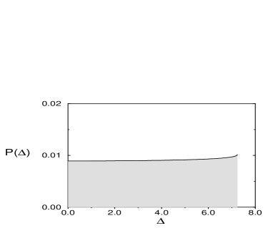
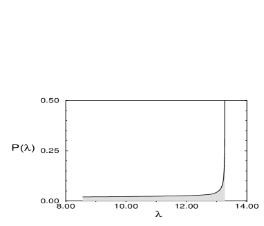
Figure 2: Distributions ${\cal P}(\Delta)$ (for positive $\Delta$), and ${\cal P}(\lambda)$ in RS. Here $\gamma=4$, while $J_{0}=0$. After [13]

We can check these assumtions against the results from our model [13]. Obviously, since the values of both $\Delta$ and $\lambda$ are determined by a single random variable, viz. $h_{\rm RS/1RSB}$, these quantities must be perfectly correlated in our model, in contrast to the assumptions of the STM, although their distributions separately are indeed rather flat, except for anomalies at their upper end (see Fig. 2) where due to large $h_{\rm RS/1RSB}$ DWPs cease to exist.

The perfect correlation can be weakended, but not eliminated, by allowing local randomness, that is, by making the coefficients $a_{2}$ and $a_{4}$ in (3) vary randomly from site to site. A randomly varying $a_{2}$ is, in fact, a natural choice in our approach, since the $a_{2}$ contribution to $U_{\rm int}$ should be considered part of the harmonic level, which we had assumed to be random to begin with. Indeed, by allowing this kind of randomness, our results can be brought into better agreement with the experimental situation (see below). As to $a_{4}$, we have observed that taking it to be random (within limits of course) has no dramatic effect, so we adhere to it remaining non–random, serving solely, as it should, its stabilising purpose. We should add that our model remains solvable with these modifications. Outer averages in the fixed point equations simply have to be read as implying an additional average over the local randomness.

As a final unexpected result, note that our theory predicts the existence under suitable circumstances of an amorphous phase without DWPs, and hence without low–energy tunneling excitations (see Fig. 1b). Until very recently, this would perhaps have universally been considered rather a surprise. However, recent internal friction measurements in specially prepared amorphous Si:H films by Liu et al. [22] indicate that such a possibility has to be seriously taken into account.

4 Thermodynamics

Information about the thermodynamics of the system at low temperatures, where it is dominated by quantum effects, is obtained by studying the excitation spectra of the local Hamiltonians (14), and by using this information — avaraging it over the randomness characterizing the ensemble of these local Hamiltonians, i.e. over the $h_{\rm RS/1RSB}$–distributions (and possibly the $a_{2}$–distribution) — to compute densities of state and thermodynamic functions the usual way.

In Fig. 3a we exhibit a typical excitation spectrum, as it varies with the value of $h_{\rm eff}$. The salient features are two kinds of branches, steeper and less steep ones. The former are related to tunneling (inter–well) excitations whereas the the latter are of intra–well type. That is, the latter would also exist if the wells were not communicating via a barrier of finite height and width. Note that these families of levels do not cross as might appear at first sight. Rather, there are avoided ‘would-be’ level–crossings precisely due to the tunneling mechanism. At at energies higher than the barrier or at large $h_{\rm RS}$ the avoided crossing–pattern disappears, because there is no longer a barrier to be tunneled through.

The corresponding density of states (DOS) (averaged over the ensemble) is displayed in Fig. 3b. Note its constant value at energies lower than that of the first intra–well excitation. It arises because, (i) apart from the immediate vicinity of its lower cutoff $\Delta_{0}$, the level–splitting of the ground–state scales linearly with the asymmetry $\Delta$, which in turn is proportional to $h_{\rm eff}$, and (ii) because the distribution of $h_{\rm eff}$ is virtually flat in this regime.

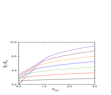
Figure 3: a): Excitation spectrum as a function of $h_{\rm RS}$. $\gamma=4$ and $J_{0}=0$. are as in Fig. 2. b): Density of states in RS, for parameters as in (a).

This energy range is to be associated with the universal glassy low–temperature anomalies below 1 K! Its properties are mainly driven by the distribution of effective fields $h_{\rm eff}$ and are thus entirely of collective origin. In particular it is related to the temperature range in which the specific heat scales linearly with temperature (see Fig. 4).

Figure 4: Specific heat at low temperatures a): without local disorder (full line RS, dashed line 1RSB) , b): with $\gamma=1$, and $a_{2}$ a Gaussian of mean 1 and variance $\sigma=5$ in RS. Other parameters are as before. The thin line corresponds to $C\sim T^{1.1}$.

By contrast, the energies of the intra–well excitations are much less sensitive to the value of the effective field, hence less steep in the excitation spectrum if plotted vs. $h_{\rm eff}$. These give rise to the strong increase of the DOS at the value of the first intra–well excitation (the contribution to the DOS being proportional to the inverse slope of the level as a function of $h_{\rm eff}$). The intra–well excitations depend more strongly on the shape of the local stabilizing potentials $G(v)$, hence they cannot be of collective origin — basically they turn out where we have chosen them to be, with or without local randomness in the $G(v)$. So the physics that depends on these features, namely the bump in $C(T)/T^{3}$ and the plateau in the thermal conductivity, cannot be expected to be universal.

This separation within our approach of aspects that can be expected to be universal from those which cannot is in perfect qualitative agreement with the experimental situation. It is not unreasonable to suppose that such a distinction between local and global contributions to $U_{\rm int}$ can be made for real materials as well, the contribution of the long–range global one being for instance of elastic nature (and well known to give rise to frustration).

Note that our representation of local potential energy configurations has finally turned out to be similar to that proposed within the SPM [7, 8] with some marked differences in the details: (i) Within our approach the very occurrence of DWPs is of identifiable collective origin, and so is the distribution of asymmetries. (ii) No analogous mechanism is available for determining (distribution of) the parameters entering $G(v)$, which are mainly responsible for the distribution of barrier heights and the nature of (single- and) intra-well excitations which determine the material–specific properties. From our vantage point, therefore, one should not even attempt at proposing for these something universally valid for all glassy materials.

There is some influence of local disorder on the behaviour of the low $T$ specific heat also in the ‘universal’ regime changing it to slightly superlinear, with exponents depending on the nature of the distribution. This feature, too, agrees nicely with experimental findings, and it might be used to give some handle at fixing the distribution of local parameters for specific materials.

Concerning universality, Yu and Leggett supposed that it could result only due to a sufficiently long range interaction between TLSs, an idea which has since the been pursued in a series of papers by Burin and Kagan [23]. Here we have seen that that it can arise without assuming interactions at the level of quantized excitations, because the statistics of local potential energies is by itself already a largely collective affair.

5 Dynamics

Let us add a few brief remarks concerning dynamics. We have in mind here the computation of phonon mean free paths, of internal friction and the thermal conductivity, the latter two computable once the phonon mean free paths are known, as well as the computation of dielectric susceptibilities. All interesting properties can be computed within linear response theory. We assume a bilinear interaction of the local coordinates $v_{i}$, whose dynamics are given by $H_{S}=H_{\rm eff}$ in (14), with the extended phonon degrees of freedom

$$H_{B}=\sum_{ks}\hbar\omega_{ks}b_{ks}^{\dagger}b_{ks}$$ (16)

that is mediated by the strain-field, and of the form

$$H_{SB}=v\sum_{s}\gamma_{s}e_{s}$$ (17)

with $s$ labelling the acoustic branches of the phonon spectrum, $e_{s}$ denoting the contribution of branch $s$ to the strain field at site $i$ and appropriate coupling constants $\gamma_{s}$. A Debeye model is assumed for the phonon bath.

The dynamic properties of interest can be computed from the imaginary part of the dynamic susceptibility $\chi^{\prime\prime}_{vv}(\omega)$, which in turn, via fluctuation dissipation theorems, is related to the (symmetrized) centered correlation function

$$\hat{C}_{vv}(t)=(\Delta v(t)|\Delta v)=\frac{1}{2}\langle\Delta v(t)\Delta v+\Delta v\Delta v(t)\rangle\ ,$$ (18)

specifically to the spectral function associated with it. Here $\Delta v=v-\langle v\rangle$. The Mori-Zwanzig Projection technique and (at this time) a weak coupling assumption are used to carry through in practice.

As of now, we have not yet produced quantitative results. So much can, however, be said at this point. In the limit of very low temperatures, our model clearly approaches the TLS-physics, and we expect a roughly quadratic temperature dependence of the thermal conductivity. The increased density of states in the 1 – 10  K range goes along with a new, and faster scattering mechanism: both are due to the existence of intra–well (as opposed to the slower inter–well) transitions in this energy range. As discussed by Yu and Leggett [11], the combination of these features can be expected to produce the plateu in the thermal conductivity. We shall report on these matters in greater detail in the near future [21].

6 Conclusions and Outlook

In summary, we have proposed to take a new look at glassy low–temperature anomalies from a model–based rather than phenomenological approach. The models so far considered do certainly not (yet) attempt to describe the details of any specific substance. Our aim has been to formulate something very schematic that should capture the essentials of amorphous low temperature phases — a caricature in the same sense as the Ising model is a caricature description of uniaxial ferromagnets or, perhaps less boldly, the SK model a prototypic description of a spin–glass. Chances are of course, that we still haven’t got the bare essentials right. But we feel that our first attempts do point in the right direction. In particular the clue we have obtained concerning the understanding as to which phenomena might be expected to be univeral and which not, does look like an encouraging general qualitative result.

Our approach offers the unique possibility to study the whole range of glassy physics, from the regime of the glass transition temperature down to the low temperatures where quantum effects play a dominant role, all within a single set of model assumptions. In particular, it should be interesting to study the glassy dynamics within the type of models we have proposed at or near their respective glass transition temperature.

Another issue concerns the classification of spin–glasses into roughly two families, one exhibiting a continuous transition and infinitely many levels of RSB, the other a discontinuous transition, and only one level of RSB, the model class we have presented here belonging to the first. There are indications that at least from the point of view of dynamics near the glass transition, the second class should be more appropriate, since it exhibits dynamic freezing transitions at temperatures higher than the thermodynamic transition temperature seen in equilibrium treatments [24]. We are currently studying a modified version of the Bernasconi model [25] in this context [26]. Finally, we have started to apply our approach to the case of defect crystals like KCl:Li to study the effects of the dipolar interaction among the Li defects at higher concentration [27], a system that has the distinct advantage that the on-site potential $G(v)$ is well known.

In the present paper we have quantised our system only after a mean–field decoupling. In principle, the analysis should start out from a full-fledged quantum-statistical formulation, using imaginary time path integrals in conjunction with the replica method. Such a formulation has been worked out [28] and will be analysed in detail in the near future. So much can be said already at this point. Our present approch amounts to investigating the quantum–statistical physics in the so–called static approximation [29]. In the present context, this approximation amounts to ignoring the feedback of quantum fluctuations on the effective single site potentials.

Acknowledgements This work has been supported by the Deutsche Forschungsgemeinschaft through the Graduiertenkolleg “Physikalische Systeme mit vielen Freiheitsgraden” (U.H.), and a Heisenberg Fellowship (R.K.). It is a pleasure to thank C. Enss, H. Horner, S. Hunklinger, M. Mézard, P. Nalbach, O. Terzidis, and A. Würger for helpful discussions and encouragement. R.K. would like to thank the Physics Department of the University of Illinois at Urbana-Champaign for its hospitality while parts of this paper were being written.

References

- [1] R.C. Zeller and R.O. Pohl, Phys. Rev. B4 2029 (1971)
- [2] J.J. Freeman and A.C. Anderson, Phys. Rev. B 34, 5684 (1986)
- [3] Phillips, J. Low Temp. Phys. 7, 351 (1972)
- [4] P.W. Anderson, B. Halperin, and S. Varma, Phil. Mag. 25, 1 (1972)
- [5] S. Hunklinger and W. Arnold, in Physical Acoustics, edited by W.P. Mason and R.N. Thurston (Academic, New York, 1976) Vol. XII, p. 155; S. Hunklinger and A.K. Raychauduri, in Progress in Low Temperature Physics, edited by D.F. Brewer (Elsevier, Amsterdam, 1986) Vol. IX, p. 267
- [6] W. A. Phillips, Rep. Progr. Phys. 50, 1675 (1987)
- [7] V.G. Karpov, M.I. Klinger, and F.N. Ignat’ev. Zh. Eksp. Teor. Fiz. 84, 760 (1983) [Sovj. Phys. JETP 57, 439 (1983)]
- [8] U. Buchenau, Yu.M. Galperin, V.L. Gurevich, D.A. Parshin, M.A. Ramos, and H.R. Schober, Phys. Rev. B46, 2798 (1992)
- [9] H.R. Schober and B.B. Laird, Phys. Rev. B 44, 6746 (1991)
- [10] A. Heuer and R.J. Silbey, Phys. Rev. Lett. 70, 3911 (1993)
- [11] C.C. Yu and A.J. Leggett, Comments Cond. Mat. Phys. 14, 231 (1988)
- [12] E.R. Grannan, M. Randeira, and J.P. Sethna, Phys. Rev. Lett. 60, 1402 (1988)
- [13] R.Kühn, in: Complex Behaviour of Glassy Systems, Proceedings of the XIVth Sitges Conference, edited by M. Rubi, Springer Lecture Notes in Physics (Springer, Berlin, Heidelberg, 1996)
- [14] R. Kühn and U. Horstmann, Phys. Rev. Lett. 78, 4067 (1097)
- [15] M. Mézard, G. Parisi, and M. A. Virasoro, Spin Glass Theory and Beyond, (World Scientific, Singapore, 1987)
- [16] T. Kirkpatrick and D. Thirumalai, J. Phys. A22, L149 (1989); J.P. Bouchaud and M. Mézard, J. Phys. I (France) 4, 1109 (1994): E. Marinari, G. Parisi, and F. Ritort, J. Phys. A27, 7615 (1994); — ibid. 7647 (1994); J.P. Bouchaud, L. Cugiandolo, J. Kurchan, and M. Mézard, Physica A226, 243 (1996)
- [17] D. Sherrington and S. Kirkpatrick, Phys. Rev. Lett 35, 1792 (1975)
- [18] J. Hopfield, Proc. Natl. Acad. Sci. USA, 81, 3088 (1984)
- [19] R. Kühn, S. Bös, and J.L. van Hemmen, Phys. Rev. A 43, 2084 (1991); R. Kühn and S. Bös, J. Phys. A 26 831 (1993); S. Bös, PhD Thesis, Gießen (1993), unpublished
- [20] J.R.L. de Almeida and D.J. Thouless, J. Phys. A 11, 983 (1978)
- [21] U. Horstmann and R. Kühn, in preparation
- [22] X. Liu, B.E. White Jr., R.O. Pohl, E. Iwanizcko, K.M. Jones, A.H. Mahan, B.N. Nelson, R.S. Crandal, and S. Veprek, Phys. Rev. Lett. 78, 4418 (1997)
- [23] A.L. Burin and Yu. Kagan, JETP 82, 159 (1996), and references therein
- [24] T.R. Kirkpatrick and D. Thirumalai, Phys. Rev. B 36 5388 (1987); A. Chrisanti, H. Horner, and H.J. Sommers, Z. Phys B 92 257 (1993)
- [25] J. Bernasconi, J. Physique, 48, 559 (1987)
- [26] J. Dimitrova and R. Kühn (1998), work in progress.
- [27] R. Kühn and A. Würger, in preparation
- [28] R. Kühn, unpublished
- [29] A.J. Bray and M. Moore, J. Phys. C 13, L655 (1980)