Dynamical properties of the Zhang model of Self-Organized Criticality

Abstract

Critical exponents of the infinitely slowly driven Zhang model of self-organized criticality are computed for $d=2,3$ with particular emphasis devoted to the various roughening exponents. Besides confirming recent estimates of some exponents, new quantities are monitored and their critical exponents computed. Among other results, it is shown that the three dimensional exponents do not coincide with the Bak, Tang, and Wiesenfeld (abelian) model and that the dynamical exponent as computed from the correlation length and from the roughness of the energy profile do not necessarily coincide as it is usually implicitly assumed. An explanation for this is provided. The possibility of comparing these results with those obtained from Renormalization Group arguments is also briefly addressed.

I Introduction

Despite more of a decade of intensive studies, the phenomenon named Self-Organized Critically (SOC) by Bak, Tang, and Wiesenfeld (BTW) [3] is far from being fully understood. The name SOC originates from the fundamental property that an open system externally driven in a (infinitely) slow fashion, settles into a critical state with no characteristic time and length scales, without any parameter tuning; see e.g. Ref. [4] for a review.

Although a large number of recipes have been proposed as toy models to mimic this behavior, the original sandpile model [3] still carries most of the information presented in this phenomenon. A variation of this model was introduced a couple of years later by Zhang [5]. The basic differences with respect to the BTW model were: first, the variable describing the state of the lattice site could take continuous rather than discrete values; second, the BTW model is abelian [6] while the Zhang model is not. In spite of this differences, extensive recent numerical simulations [7] on the two-dimensional Zhang model, opened the possibility that they both belong to the same universality class, in disagreement with the original scaling prediction by Zhang [5]. Apart from the aforementioned investigation [7], the Zhang model was already studied in different dimensionalities in Ref. [8] where an estimates for some critical exponents, notably the avalanche size exponent $\tau_{s}$, was given. However, these estimates, whose main aim was to test the robustness of universality of the model under anisotropy of the energy repartition, appeared to be based on small sizes and statistics.

On the other hand, a Langevin counterpart of the Zhang model was repeatedly studied by Renormalization Group (RG) methods [9, 10, 11, 12], and predictions for critical exponents in a one-loop working scheme were drawn. The dynamical exponent $z$ as calculated from the correlation function in the case when the additive noise has a typical time scale much bigger than the relaxation time scale [10], turned out to be very close to the one relating the correlation length and the relaxation time in the standard dynamical scaling hypothesis [13] in the Zhang model.

It is then desirable to have a more complete numerical investigation touching upon those issues appearing in the RG calculations and those which were previously neglected. This is indeed the aim of the present work where a fairly complete analysis of the model, in different dimensionalities is carried out and compared, when possible, with previous numerical and RG work. By doing this we found few unexpected results.

Firstly, the three-dimensional results do not support the conjecture that the Zhang and the BTW models belong to the same universality class. Secondly, whereas it is true that the exponent $z$ of the Zhang model is very close to the one obtained by RG techniques as previously discussed, the roughening exponent is not [10]. Finally, the critical exponent $z$ is different when calculated from the dynamical scaling ansatz and when computed from the roughness exponent. This latter discrepancy can be fixed in our case by noting that the correlation length (maximum avalanche distance) does not scale linearly with system size $L$.

The plan of the paper is as follows. In Sec. II the model is defined, whereas in Sec. III all relevant quantities concurring to identify the critical behavior of the model are laid down. Sec. IV contains the results of this effort and comparisons with earlier ones, and finally some conclusive remarks are left in Sec. V.

II The slowly driven Zhang model

Each point of an hypercubic lattice is characterized by a continuous energy variable $E_{\tau}({\bf x},t)$, where ${\bf x}$ denotes the lattice position, $t$ the driving (slow) time, and $\tau$ the relaxation (fast) time. Whereas $t$ runs from 0 to a sufficiently large value needed to get good statistics, $\tau$ runs from 0 to $T(t)$, which is the total fast time that an avalanche initiated at a slow time $t$ takes to be completed. In this way the two time scales are well separated. Starting from an initially empty lattice, the dynamics of the evolution is defined as follows [5]:

1. Start with a randomly chosen lattice point ${\bf x}_{0}$ and set it slightly above some critical energy $E_{c}$ (hereafter chosen to be $1$ without loss of generality) by repeated addition of a random energy taken uniformly from the interval $(0,1/4)$ [14, 15].

2. The site ${\bf x}_{0}$ relaxes according to the following equation:

   $$E_{\tau+1}({\bf x},t) = [1-\theta(E_{\tau}({\bf x},t)-E_{c})]E_{\tau}({\bf x},t)+$$ (1)

   $$+ \frac{1}{2d}\sum_{{\bf y}({\bf x})}\theta(E_{\tau}({\bf y},t)-E_{c})\;E_{\tau}({\bf y},t)$$ (2)

   where $\theta(\cdot)$ is the Heaviside step function and $d$ is the space dimension. Here the notation $\sum_{{\bf y}({\bf x})}$ means that the sum is restricted to the nearest-neighbors ${\bf y}$ of site ${\bf x}$. Clearly this is tantamout to say that each site ${\bf x}$ whose energy exceeds a critical value $E_{c}$ is set to zero and its energy is equally redistributed to the nearest-neighbors.

3. Iterate Step 2 for the other sites that become critical until all sites are below $E_{c}$.

4. At this point increase $t$ by one unit ($t\rightarrow t+1$), and randomly pick a new initial seed ${\bf x}_{0}^{\prime}$ in Step 1.

The process is iterated until the system has reached a steady-state configuration where the average energy

$$\overline{E(t)} = \frac{1}{V}\sum_{{\bf x}}E({\bf x},t)$$ (3)

reaches a well defined value. Here $V=L^{d}$ is the volume of the lattice. We note that whenever there is no subscript for the energy it will be implicitly assumed that the avalanche is over, i.e. $\tau$ has reached $T(t)$. Starting at this time, when the system has reached a stationary state, we collect all the relevant dynamical properties.

III Probability distributions and correlation functions

At each time $t$ there is a growing avalanche; within the fast time scale we can measure the number of active sites at each update ($\tau$)

$$S_{\tau}(t)=\sum_{{\bf x}}\theta(E_{\tau}({\bf x},t)-E_{c})$$ (4)

and from this we can define the size of an avalanche at time $t$

$$S(t)=\sum_{\tau=1}^{T(t)}S_{\tau}(t).$$ (5)

From the size of the avalanche we can compute a characteristic length $\xi(t)$ defined as the radius of gyration with respect to the seed site ${\bf x}_{0}$. This characteristic length is related to the time the avalanche needs to be completed through the standard relation [13]

$$T(t)\sim\xi^{z}(t)$$ (6)

which defines the dynamical exponent $z$.

Other quantities that are interesting to measure are the total input and output currents. They are defined as follows

$$J_{\mbox{{in}}}(t) = \delta E({\bf x}_{0},t)$$ (7)

$$J_{\mbox{{out}}}(t) = \sum_{\tau=0}^{T(t)}\sum_{{\bf x}\in\partial\Lambda}E_{\tau}({\bf x},t)$$ (8)

where $\Lambda$ is the bulk and $\partial\Lambda$ is the boundary of the bulk (the sum of the two forming the total available lattice space). Here $\delta E({\bf x}_{0},t)$ is the total added energy necessary to the site to be active (i.e. above the critical energy $E_{c}=1$).

In order to take into account the existence of two different time scales one should be very careful when defining the correlation functions. Upon extending (3), we can define the $q-$th spatial moment of the energy as

$$\overline{E^{q}}(t) = \frac{1}{V}\sum_{{\bf x}}E^{q}({\bf x},t)$$ (9)

and then the interface width (or roughness) [16] is

$$W_{s}(t,L) = \sqrt{\overline{E^{2}(t)}-\overline{E(t)}^{2}.}$$ (10)

This definition applies to the slow time scale as also indicated by the suffix $s$, and coincides with the usual definition of roughness in the framework of growth processes. On the other hand one could think to measure the energy fluctuations during the evolution of an avalanche. Since an avalanche of duration $\tau$ occurs at many different input times $t$, we define the following fast roughness:

$\displaystyle W_{f}^{2}(\tau,L)=$

$$=<\frac{1}{V}\sum_{{\bf x}}E_{\tau}^{2}({\bf x},t)-\left(\frac{1}{V}\sum_{{\bf x}}E_{\tau}({\bf x},t)\right)^{2}>_{t}.$$ (11)

In Eq. (11) the roughness is averaged over different times $t$ (and hence avalanches).

According to standard scaling hypothesis (see e.g. [16]) one expects these correlation functions to display the following scaling forms:

$$W_{f}(\tau,L)=\tau^{-\beta_{f}}\Phi_{f}(\tau/L^{z_{f}})$$ (13)

$$W_{s}(t,L)=t^{\beta_{s}}\Phi_{s}(t/L^{z_{s}})$$ (14)

where $\Phi_{f}$ anf $\Phi_{s}$ are finite size functions.

In (13) the roughness is expected to decrease rather than to increase as in more conventional growth processes [16], because the maximum energy is bounded and the avalanche is a relaxational process.

IV Critical exponents and Results

This model was already carefully investigated in two-dimensions. Apart from the original work [5], recent extensive simulations on remarkably large sizes were carried out in $d=2$[7]. When comparable, our results are in good agreement with both previous analysis. However, in these papers, the behavior of some important quantities, necessary to our purposes, were neglected, nor was a complete study in dimensionality different from $2$ ever attempted. Indeed while Zhang only reported the steady state value of the average energy along with the ”quantized” energy distribution $P(E)$ for $d=3$, in [8] a value for the avalanche size exponent (see below) is reported for dimensions up to $4$. The latter was however probably based on very small sizes without any attempt of a finite scale analysis. As a result these estimates, albeit close, turn out to be slightly off compared to ours.

In our simulations we used sizes up to $L=300,60$ and times up to $2^{17},2^{18}$ in $d=2,3$ respectively. These are smaller than the ones used in [7] for $d=2$ but considerably larger than all other three dimensional studies.

For the sake of clarity and compactness, let us now review some known results first. As it is well known by now, the system reaches a steady state (where the average energy is no longer changing) after a transient which clearly scales as $L^{d}$ since it takes that many time steps (on average) to ”explore” the whole lattice. The resulting values of the stored energy $\overline{E(t)}$ are $0.63\pm 0.01$ and $0.58\pm 0.01$ (estimated from the largest sizes) in $d=2,3$ respectively. These results are in agreement with those found by Zhang in his original simulations. Another feature already observed by Zhang is that the critical state has energy which is peaked around well defined energies the number of which depends only on the dimensionality of the hypercubic lattice. It has also been established that this feature is unchanged upon introducing an asymmetry in the probability distribution and by introducing different lattices [8].

As explained by Hwa and Kardar [17] in the framework of the one-dimensional BTW sandpile model, monitoring the total output energy current proves to be very useful in understanding the mechanism that leads to the steady state. This is shown in Fig. 1. Whereas clearly the input current is a random function between 0 and 1, the output current displays sequences of bursts followed by long periods of quiescence similar to the one found by Hwa and Kardar in the slow driving regime. We also computed its power spectrum $S({\nu})$ (the Fourier transform of the output current-current correlation) which appears to be white noise in all cases. This is related with the fact that our system corresponds to a non-interacting avalanche regime in their language [17].

We now turn to the calculus of critical exponents. First we consider the exponent $z$ as defined in (6). This was computed by plotting the average duration of the avalanches as a function of their characteristic average lengths. A binning procedure analogue to the one used in [9] was employed. Plots are shown in Fig. 2. Our best fit estimates are $1.34\pm 0.02$ and $1.65\pm 0.02$ in $d=2,3$ respectively, compatible with the BTW values which are $4/3$ and $5/3$. Remarkably, these results are also in perfect agreement with the RG results of Ref. [12] which are $1.36\;(d=2)$ and $1.68\;(d=3)$. The RG analysis was performed on a Langevin equation where the driving and the relaxation time scales are comparable (and hence not well separated). Furthermore the strong (infinite) non-linearity appearing in the continuum analogue of Eq. (1), was regularized and the result was analyzed within a one-loop RG scheme. In view of all these approximations, the aforementioned closeness in the two results is rather surprising. We shall come back to this issue later on.

Another interesting critical exponent is the avalanche exponent size $\tau_{s}$ defined by the relation

$$p(S) = S^{-\tau_{s}}F(S/L^{\phi}).$$ (15)

Here $p(S)$ is the distribution density of the avalanche sizes $S$, $\tau_{s}$ is the avalanche exponent and $F(x)$ is a finite size function defining the exponent $\phi$ [18]. The function $F(x)$ is assumed to go to a constant for small arguments (i.e. large sizes $L$) and to ”regularize” the large avalanche behaviour. In order to improve the numerical estimates it proves convenient to look at the integrated distribution density defined as

$$P(S) = \int_{0}^{S}\;ds\;\;p(s).$$ (16)

We have estimated the values of $\tau_{s}$ in two different ways. By plotting the local slope (Fig. 3) and upon a finite size procedure (analogue to the one used in Refs. [7] and [19], see Fig. 4). Both procedures yield consistent results. In $d=2$ our best estimate is $1.288\pm 0.019$ which is close to the one given in Ref [7] by Lübeck, who reports $1.282\pm 0.010$. It appears however that the two extrapolations are not identical, since in his analysis the values are increasing as $L$ increases rather than decreasing as one would expect from a finite size scaling.

Remarkably, both values are in good agreement with the BTW value, thus supporting the claim that the Zhang model belongs to the BTW universality class [7]. Our $d=3$ result is $1.454\pm 0.041$ and it supersedes the one reported by Janosi [8] namely $1.55$ which was presumably based only on small sizes (and thus too high according with our previous discussion). However this disagrees with the BTW value $4/3$ (see e.g. [19]) and hence with the claim that the BTW and Zhang model belong to the same universality class.

The values of $\phi$ were computed from the collapse of the curves obtained plotting $S^{\tau_{s}}\;P(S)$ versus $S/L^{\phi}$, that is the universal finite size function. We find the best collapse for $1.80\pm 0.05$ and $2.6\pm 0.1$. The error bars are estimated graphically. A consistent value can be estimated by plotting the size of the maximum avalanche as a function of the size $L$, which is expected to scale as:

$$s_{\mbox{max}} \sim L^{\phi}.$$ (17)

A log-log linear fit yields $1.84\pm 0.06$ ($d=2$) and $2.54\pm 0.09$ ($d=3$). A summary of all these critical exponents is reported in Tables I and II.

Let us now turn to the behavior of the roughness as defined in Eqs. (14). As mentioned earlier, the dynamical exponent $z$ can be found from the scaling ansatz (6). However, as it is usually done in the field of growth processes [16], one might think to derive it from the scaling of the roughness as well. In Fig  5 we plot the roughness as defined in (11). We find (13) to hold true with $\beta_{f}=0.282\pm 0.013$ and $\beta_{f}=0.391\pm 0.031$ in $d=2,3$ respectively. These values were obtained upon using an analysis similar to the one exploited to compute $\tau_{s}$. From the collapse plot one can then infer the value of $z_{f}$ appearing in (13). We find $z_{f}=1.20\pm 0.05$ $(d=2)$ and $z_{f}=1.4\pm 0.1$ $(d=3)$, which are both lower than the corresponding value derived from (6). Similarly to (17) we have that

$$T\sim L^{z_{f}}$$ (18)

with $z_{f}=1.19\pm 0.04$ ($d=2$) and $z_{f}=1.34\pm 0.04$ ($d=3$). Commonly the equality $z=z_{f}$ is tacitly assumed to hold and we are not aware of any other examples where this point was sufficiently emphasized. A simple argument can be given here to explain this discrepancy. In usual interface growth phenomena the dynamical exponent is measured as the scaling of the saturation time with the system length, and this saturation occurs when the correlation length reaches the system length. In our case, both lengths do not scale linearly but as $\xi\sim\L^{\eta}$. Thus these exponents need not be identical unless $\eta=1$. By a direct measurement (looking on how the maximum $\xi$ scales with $L$) we have found that $\eta=0.922\pm 0.012$ and $\eta=0.897\pm 0.051$, for $d=2$ and $3$, respectively. According to these scaling arguments we find that the product $z\eta$ agrees, within error bars, with the values reported for $z_{f}$. In certain surface growth models a similar phenomenon, called anomalous scaling, has been reported [20]. There it has been observed that the roughening exponents are different when measuring the local or the global widths.

Another exponent is derived from the relation $\chi_{f}=\beta_{f}\;z_{f}$ which is telling that the roughness, after that the avalanche has been completed (i.e. at time $T(t)$), decreases as $L^{-\chi_{f}}$. The values $\chi_{f}=\beta_{f}\;z_{f}$, according to our previous results, are $0.33$ and $0.55$ in $d=2,3$ respectively. We now go back to the comparison with the RG results.

As previously hinted, although the exponent $z$ derived from (6) is very close to the one derived by RG methods on the continuum Langevin analogue of the Zhang model [10], the $\beta_{f}$ and $\chi_{f}$ exponents are not. A summary of all these values is reported in Table III for compactness. We argued previously that this inconsistency is not surprising in view of the different physical regimes probed by the two cases and of the heavy approximations involved in the RG calculation. The apparent equality in the dynamical exponent $z$ then probably hinges on deeper and more interesting reasons, and we are planning to consider this in a future work.

Finally, we have also measured the roughness on the slow time scale as defined by (10). We find that after a transient scaling as $L^{d}$, the roughness tends to a limit which is independent on $L$ (see Fig. 6), i.e. eq. (14) holds with $\beta_{s}=0$, $\chi_{s}=0$ and $z_{s}=d$.

V Conclusions

In this paper we have studied the infinitely slowly driven Zhang model in two and three dimensions. In two dimensions this work can be seen as a complement of an earlier large sizes study [7]. On the other hand in three dimensions, our results are expected to improve an earlier estimate[8]. The aim of [8] was different from ours and this could account for the difference. In both cases we computed some exponents (notably the $\phi$ and all the roughness exponents) which were never previously considered. Besides being an useful complement to the existing literature on the model we also found few unexpected results: i) the three dimensional avalanche size exponent does not coincide with the BTW value, as the two-dimensional value seems to suggest; ii) the exponent $z$ computed from the dynamical scaling ansatz does not coincide with the one computed from the roughening exponent. We have shown that this stems from the non-linear scaling of the correlation length $\xi$ with the system size $L$; iii) the coincidence between the value of $z$ of the Zhang model and the RG value derived on its Langevin continuum counterpart, does not extend to other exponents such as the $\beta$ and the $\chi$ exponent.

We believe that all the above issues deserve further attention both from the analytical and numerical view point. We are currently performing a numerical investigation on the continuum Langevin equation. This further analysis is expected to shed new lights on the approximations involved in the RG treatment.

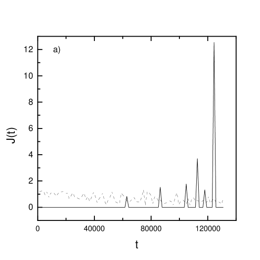
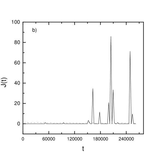
FIG. 1.: Plot of the total energy $J(t)$, both in (dotted line) and out (full line), in $d=2$ (a) and $d=3$ (b).

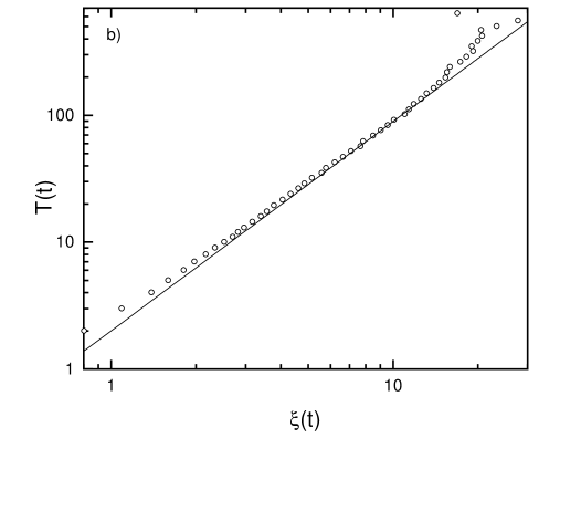
FIG. 2.: Log-Log plot of the relation $T\sim\xi^{z}$ in $d=2$ (a) and $d=3$ (b). The full line corresponds to the value reported in Table II.

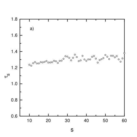
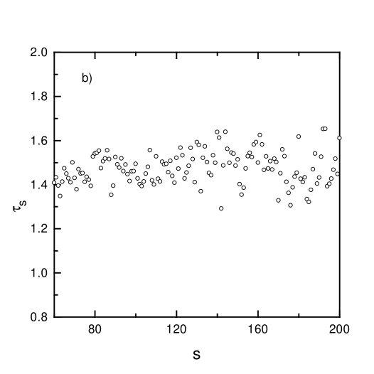
FIG. 3.: Local slope plot for $\tau_{s}$ as a function of the avalanche size $S$ in $d=2$ (a) and $d=3$ (b). In both cases the intermediate most linear part of the largest size was used for the computation.

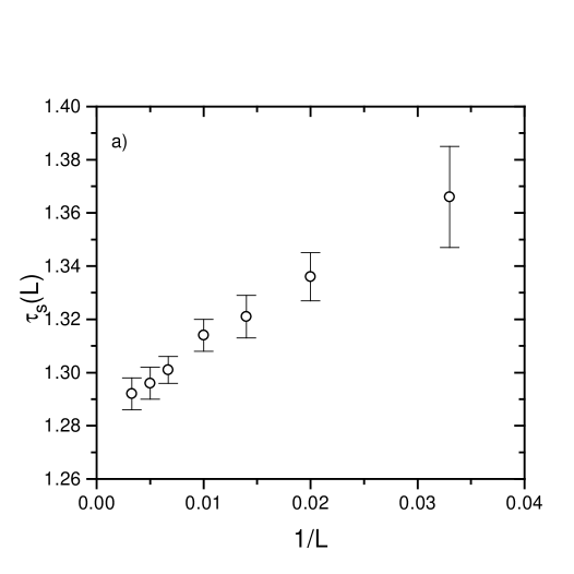
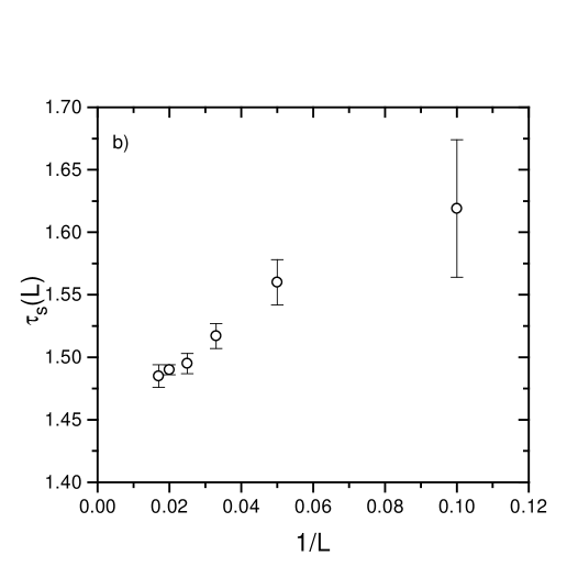
FIG. 4.: Finite size plot for $\tau_{s}$ as a function of the inverse lattice size $1/L$ in $d=2$ (a) and $d=3$ (b).

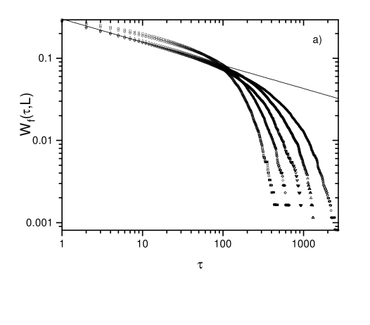
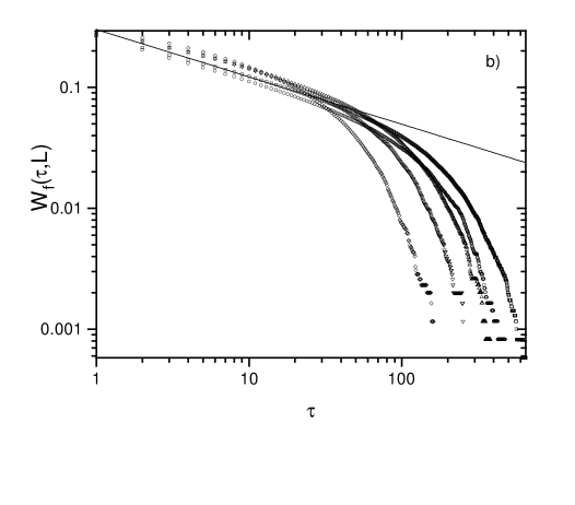
FIG. 5.: Log-Log plot of $W_{f}(\tau,L)$ as function of $\tau$ for various sizes $L$. In $d=2$ these were $L$=70 ($\Box$), 100 ($\diamond$), 150 ($\nabla$), 200 ($\triangle$), 300 ($\circ$), and in $d=3$ they were $L$=20 ($\diamond$), 30 ($\nabla$), 40 ($\triangle$), 50 ($\circ$), 60 ($\Box$). In both cases the solid line corresponds to the value of $\beta_{f}$ reported in Table III.

FIG. 6.: Plot of $W_{s}(t,L)$ as function of $t$ for various sizes $L$ both for $d=2$ (a) and $d=3$ (b). The values used for the sizes are the same of the previous figure, the larger $L$ the slower the growth.

TABLE I.: Critical exponents $\tau_{s}$ and $\phi$ in $d=2,3$. The values indicated by (a) and (b) refer to the BTW [19] and the previous works [7, 8], respectively. The exponent $\phi$ given here is computed from (17).

$d$	$\tau_{s}$	$\tau_{s}(a)$	$\tau_{s}(b)$	$\phi$	$\phi(a)$	$\phi(b)$
2	$1.288\pm 0.019$	$1.293$	$1.282\pm 0.010$	$1.84\pm 0.06$	2	-
3	$1.454\pm 0.041$	4/3	1.55	$2.54\pm 0.09$	3	-

TABLE II.: Dynamical critical exponent in $d=2,3$. The first column corresponds to (5), whereas the second column is computed from (15). Finally the last two columns indicated by (a) and (b) are the BTW [19] and the RG values [10], respectively.

$d$	$z$	$z_{f}$	$z(a)$	$z(b)$
2	$1.34\pm 0.02$	$1.19\pm 0.04$	4/3	1.36
3	$1.65\pm 0.02$	$1.34\pm 0.04$	5/3	1.68

TABLE III.: Roughness exponents $\beta$ and $\chi$ in $d=2,3$. The values $\beta_{f}$ and $\chi_{f}=\beta_{f}\;z_{f}$ are computed here while the others are the RG values [10].

$d$	$\beta_{f}$	$\beta$	$\chi_{f}$	$\chi$
2	$0.282\pm 0.013$	-0.26	$0.33\pm 0.03$	-0.36
3	$0.391\pm 0.031$	-0.1	$0.55\pm 0.08$	-0.18