Room temperature Kondo effect in atom-surface scattering: dynamical $1/N$ approach

Abstract

The Kondo effect may be observable in some atom-surface scattering experiments, in particular, those involving alkaline-earth atoms. By combining Keldysh techniques with the NCA approximation to solve the time-dependent Newns-Anderson Hamiltonian in the $U\rightarrow\infty$ limit, Shao, Nordlander, and Langreth found an anomalously strong surface-temperature dependence of the outgoing charge state fractions. Here we employ a dynamical $1/N$ expansion with a finite Coulomb interaction $U$ to give a more realistic description of the scattering process. We test the accuracy of the $1/N$ expansion in the $N=1$ case of spinless fermions against the exact independent particle solution. We then compare results obtained in the $U\rightarrow\infty$ limit with the NCA approximation at $N=4$ and recover qualitative features already found. Finally, we analyze the realistic situation of Ca atoms with $U=5.8$ eV scattered off Cu(001) surfaces. Although the presence of the doubly-ionized Ca⁺⁺ species can change the absolute scattered Ca⁺ yields, the temperature dependence is qualitatively the same as that found in the $U\rightarrow\infty$ limit. One of the main difficulties that experimentalists face in attempting to detect this effect is that the atomic velocity must be kept small enough to limit kinematic smearing of the Fermi surface of the metal.

I Introduction

The interaction of a localized spin impurity with the conduction electrons of a metal is a well known and interesting problem[1]. The Kondo effect arises as a result of the interaction, and thermodynamic properties such as susceptibility and specific heat have been thoroughly studied for many years, both theoretically and experimentally[2, 3, 4]. Non-equilibrium properties of these systems, however, are not well understood.

Recent advances in the construction of small quantum dots permit a high degree of control in the coupling between localized and extended electronic states. Measurements of transport through dots give clear evidence for the Kondo effect.[5] Shao, Nordlander, and Langreth (SNL) recently pointed out[6] that atomic scattering off metal surfaces is another arena for the Kondo effect. The rich variety of atomic levels, workfunctions, and couplings permits the investigation of many regimes. For example, as it encounters the surface, an atom can evolve from the empty orbital regime into the local moment regime, passing through the mixed valence state at intermediate distances from the surface. Strikingly, the Kondo scale can easily attain room temperature because the atomic level crosses the Fermi energy. The velocity of the incoming ion may also be tuned to probe the different regimes. However, only at sufficiently small velocities is there enough time for a well-developed Kondo resonance to form. The Kondo screening cloud manifests itself in enhanced neutralization probabilities at low speeds and reduced temperatures.

One theoretical approach used to analyze highly non-equilibrium atom-surface systems is the Keldysh Green’s function technique[7, 8], combined with the Non-Crossing Approximation (NCA)[9, 10]. This approach typically takes the repulsive Coulomb interaction strength $U$ between electrons residing on the impurity or scattered atom to be infinite. Although NCA has been extended to treat the case of finite $U$, at least in the static case[11], it can only be easily applied to the dynamical problem in the $U\rightarrow\infty$ limit. However, renormalization group (RG) calculations show that the parameters of the system in the finite-$U$ case[12, 13] can differ significantly from those in the $U\rightarrow\infty$ limit; in particular the Kondo temperature depends on $U$. Thus physically reasonable values for $U$ should be used in realistic calculations. Finally, NCA has additional problems as it neglects vertex corrections. Fermi liquid relations are not recovered at zero temperature. Instead spurious behavior shows up in the spectral density of the impurity[14].

In this article we present an alternative approach, namely, the dynamical $1/N$ method. Details of the method have been presented in [I][15]. Both resonant and Auger processes can be treated in the same framework, as can finite $U$. The method has been used to study charge transfer between alkali ions, such as Li and Na, and metal surfaces. Semiquantitative predictions of Li(2p) excited state formation and final charge fractions agree well with experiment[16, 15, 17], in contrast with independent particle theories which ignore the essential electron-electron correlations. Here we extend the previous work of [I] by including a new sector in the wavefunction which describes the amplitude for two particle-hole excitations in the metal. As this sector is of order $1/N^{2}$ the accuracy of the expansion is improved. A further extension of the solution permits treatment of non-zero substrate temperature.

This paper is organized as follows: In Sec. II we briefly discuss the theory and its new features. In Sec. III we present results in both the $U\rightarrow\infty$ limit and in the physical finite-U case. The $U\rightarrow\infty$ limit is studied for the purpose of comparing our $1/N$ results at $N=4$ with previously published NCA results[6]. As a further test of the $1/N$ expansion we also present results extended down to the spinless $N=1$ limit. In this case, there are exact independent particle results which can be used to test the accuracy of the $1/N$ expansion. Finally, the physically relevant case of finite-$U$ and $N=2$ is examined to determine whether or not Kondo effects are accessible to charge transfer experiments. We conclude in section IV with a discussion of the conditions which must be satisfied in charge transfer experiments which search for the Kondo effect.

II Theoretical background

Independent-particle descriptions of charge transfer fail to account for many interesting and non-trivial phenomena. Here we briefly review the main features of correlated model we employ and its approximate $1/N$ solution. Details can be found in [I][15].

A The model

Our model for atom-surface system is the generalized time-dependent Newns-Anderson Hamiltonian. For concreteness we first consider the case of alkali atoms, and then later show how a particle-hole transformation permits the description of alkaline-earth atoms. To organize the solution systematically in powers of $1/N$, the atomic orbital is taken to be $N$-fold degenerate. The physical case of electrons with up and down spins can then be studied by setting $N=2$.

$$H(t) = \sum_{a}[\epsilon^{(1)}_{a}(z)\hat{P}_{1}+\epsilon^{(2)}_{a}(z)\hat{P}_{2}]~{}\ c_{a}^{{\dagger}\sigma}c_{a\sigma}+\sum_{k}\epsilon_{k}\ c_{k}^{{\dagger}\sigma}c_{k\sigma}$$ (1)

$$+ N^{-1/2}\sum_{a;\ k}\{[V^{(1)}_{a;k}(z)\hat{P}_{1}+V^{(2)}_{a;k}(z)\hat{P}_{2}]\ c_{a}^{{\dagger}\sigma}c_{k\sigma}+H.c\}$$ (2)

$$+ {{1}\over{2}}~{}\sum_{a}U_{aa}n_{a}(n_{a}-1)+\sum_{a>b}U_{ab}n_{a}n_{b}~{}.$$ (3)

where the indices $a$ labels the discrete set of atom states and $k$ labels the continuum of electron states in the metal. Projection operators $\hat{P}_{1}$ and $\hat{P}_{2}$ project respectively onto the one and two electron subspaces and can be written explicitly in terms of the occupation number operators. Implicit summation over repeated raised and lowered spin indices, $\sigma=1,2,\cdots,N$, is assumed.

Parameters $\epsilon_{a}^{(1)}(z)$, $\epsilon_{a}^{(2)}(z)$, $V_{a;k}^{(1)}(z)$ and $V_{a;k}^{(2)}(z)$ are, respectively, the orbital energies and matrix elements for 1 and 2 electrons. The use of the projector operators enable us to use different couplings depending on the number of electrons in the atom. The couplings are divided by the square root of the degeneracy $\sqrt{N}$ so that the atomic width $N\Gamma$ remains finite and well-defined in the $N\rightarrow\infty$ limit. As excited states of the atom with two electrons occupy orbitals high in energy they are excluded. We therefore take $U_{ab}\rightarrow\infty$ when $a\neq 0$ and $b\neq 0$. In the limit $U=U_{00}\rightarrow\infty$ the above Hamiltonian reduces to a simpler, but still nontrivial, form as now the atom can be occupied by at most one electron:

$$H(t) = \sum_{a}\epsilon^{(1)}_{a}(z)~{}\hat{P}_{1}~{}c_{a}^{{\dagger}\sigma}c_{a\sigma}+\sum_{k}\epsilon_{k}\ c_{k}^{{\dagger}\sigma}c_{k\sigma}$$ (4)

$$+ N^{-1/2}\sum_{a;\ k}\{V^{(1)}_{a;k}(z)~{}\hat{P}_{1}~{}c_{a}^{{\dagger}\sigma}c_{k\sigma}+H.c\}$$ (5)

Setting $U=0$ and $N=1$ in Eq. (3), on the other hand, yields the spinless independent-particle Newns-Anderson Hamiltonian[18, 19].

Explicit time dependence enters through the classical ion trajectory. As the ion’s kinetic energy is typically much larger than the electronic energy, the trajectory to a good approximation may be considered fixed. Thus the distance of the ion away from the surface may be written simply as:

$$z(t) = z_{f}-u_{i}~{}t;\ \ \ t\leq t_{turn}\equiv(z_{f}-z_{0})/u_{i}.$$ (7)

$$= z_{0}+u_{f}~{}(t-t_{turn});\ \ \ t>t_{turn}.$$ (8)

In words, at time $t=0$ an incoming atom at position $z=z_{f}$ moves at perpendicular velocity $u_{i}$ towards the surface. At the turning point, $z=z_{0}$ it reverses course and leaves with velocity $u_{f}$. We also consider trajectories which start from the surface at $t=0$ and $z=z_{0}$. Perpendicular incoming and outgoing velocities $u_{i}\geq u_{f}$ can differ to account for loss of kinetic energy during the collision. We assume in the following that energy deposited as lattice motion is decoupled from the electronic degrees of freedom, at least over the relatively short time scale of the atom-surface interaction.

The energy of a neutral alkali atom relative to the Fermi energy, which we denote by $E[A^{0}]$, shifts due to the image potential and saturates close to the surface:

$$E[A^{0}] = {\epsilon^{(1)}_{a}(z)}=W-I_{a}+(1/V_{maxI}^{2}+16(z-z_{im})^{2}/e^{4})^{-1/2},\ \ \ z>z_{im}$$ (9)

$$= W-I_{a}+V_{maxI},\ \ \ z<z_{im}$$ (10)

Here $I_{a}$ is the ionization energy required to remove one electron from the a-orbital, $W$ is the workfunction and $V_{maxI}$ is the maximum image shift of the atomic level as it approaches the surface.

It is important to notice that in the Hamiltonian of Eq. (3), the unoccupied atomic state, $A^{+}$, is defined to have zero energy so that it is $E[A^{0}]$ and not $E[A^{+}]$ which shifts. Likewise the energy of the doubly-occupied configuration does not shift as the energy required to convert a negative alkali ion into a positive ion is constant at all distances from the surface. Thus the combination $2\epsilon^{(2)}_{a}(z)+U_{aa}$ is independent of $z(t)$ and we obtain simply:

$$\epsilon^{(2)}_{a}=W-I_{a}\ .$$ (11)

Finally the Coulomb interaction can be expressed as the difference between the affinity and the ionization levels: $U\equiv U_{00}=A+I_{0}$, where the affinity is a negative quantity.

B The model for alkaline-earth atoms

While a free alkali atom, say Li, has one electron in the valence s-orbital, Li($2s^{1}$), an alkaline-earth atom, say Ca, has a filled s-shell configuration, Ca($4s^{2}$). Due to the image potential, the neutral Li atom tends to ionize by transfer of its valence electron close to the Cu surface, yielding the closed-shell configuration $Li^{+}(1s^{2})$. In contrast, the most probable state of a Ca atom close to the surface is $Ca^{+}(4s^{1})$ which has an unpaired spin in the valence orbital. This difference is what makes the alkaline-earth atoms interesting candidates for revealing the properties of the Kondo screening cloud near metal surfaces. We may easily treat the case of alkaline-earth atoms (denoted by AE) within the wavefunction ansatz discussed below in the next subsection by performing a particle-hole transformation. This canonical transformation is implemented by switching all of the electron creation and annihilation operators: $c_{a}\rightarrow-c^{+}_{a}$, $c^{+}_{a}\rightarrow-c_{a}$, $c_{k}\rightarrow c^{+}_{k}$, and $c^{+}_{k}\rightarrow c_{k}$. Minus signs have been introduced to keep the $V_{a;k}$ matrix elements invariant. If $\epsilon_{k}$ is particle-hole symmetric as we assume, the transformation leaves the Hamiltonian unchanged up to an irrelevant additive constant as long as the energy of the atomic orbital is also reversed in sign. Thus $\epsilon^{(1)}_{a}$ should now be interpreted as the energy time of one hole in the s-orbital of the atom, corresponding to a positive alkaline-earth ion, $AE^{+}$. In this case it is appropriate to set the energy of the neutral atom to zero, $E[AE^{0}]=0$. Also the image shift is reversed in sign. Again taking into account image saturation close to the surface, the level variation as a function of distance is given by:

$$E[AE^{+}] = {\epsilon^{(1)}_{a}(z)}=I_{a}-W-(1/V_{maxI}^{2}+16(z-z_{im})^{2}/e^{4})^{-1/2},\ \ \ z>z_{im}$$ (12)

$$= I_{a}-W-V_{maxI},\ \ \ z<z_{im}.$$ (13)

The total energy of the two-hole configuration, $AE^{++}$, then shifts like

$$E[AE^{++}] = {2\epsilon^{(2)}_{a}(z)}+U=2(I_{a}-W)+U-4(1/V_{maxII}^{2}+16(z-z_{im})^{2}/e^{4})^{-1/2},\ \ \ z>z_{im}$$ (14)

$$= 2(I_{a}-W)+U-4V_{maxII},\ \ \ z<z_{im}.$$ (15)

Here $V_{maxI}$ and $V_{maxII}$ are respectively the maximum shifts in the one and two-hole orbital energies. Far from the surface, the doubly-ionized level shifts four times as much as the singly ionized level. Consequently it can play an important role even when $U$ is rather large.

C Approximate solution of the model

The time-dependent many-body wavefunction is systematically expanded into sectors which contain an increasing number of particle-hole pairs in the metal. Amplitudes for sectors with more and more particle-hole pairs are reduced by powers of $1/N$. This approach was used with success by Varma and Yafet[20] and by Gunnarsson and Schönhammer[21, 22], to describe the static ground state properties and spectral densities of metal impurities such as Ce. It was first applied to the dynamical problem in 1985 by Brako and Newns[23]; three sectors were included in this pioneering work. Subsequent work work extended this ansatz[24, 16, 15]. The improved ansatz for our wavefunction now has six sectors (for details, see [I]):

$$|\Psi(t)\rangle = f(t)|0\rangle+\sum_{a;\ k}b_{a;k}(t)|a;k\rangle+\sum_{k,\ L}e_{L,k}(t)|L,k\rangle+\sum_{q<k}d_{k,q}(t)|k,q\rangle$$ (16)

$$+ \sum_{a;\ L,\ q<k}s_{a;L,k,q}(t){|a;L,k,q\rangle}^{S}+\sum_{a;\ L,\ q<k}a_{a;L,k,q}(t){|a;L,k,q\rangle}^{A}$$ (17)

$$+ \underbrace{\sum_{L>P,\ q<k}g_{L,P,k,q}(t){|L,P,k,q\rangle}^{S}+\sum_{L>P,\ q<k}h_{L,P,k,q}(t){|L,P,k,q\rangle}^{A}}_{new~{}sector}$$ (18)

$$+ \{rest\ of\ Hilbert\ space\}\ .$$ (19)

Here $|0\rangle$ represents the unperturbed filled Fermi sea of the metal and either an empty alkali valence orbital ($A^{+}$) or a filled alkaline-earth orbital ($AE^{0}$). As the Hamiltonian conserves spin, the many-body wavefunction describes the spin singlet sector of the Hilbert space. The physical meaning of each of the amplitudes differs for alkali and alkaline earth atoms. For alkalis $e_{L,k}(t)$ is the amplitude for a positive ion with an empty valence shell, one electron in state $L>k_{F}$ of the metal, and one hole in state $k<k_{F}$ of the metal where $k_{F}$ is the Fermi momentum. For alkaline-earths, on the other hand, $e_{L,k}(t)$ is the amplitude for a neutral atom with a filled s-orbital, an electron in state $k>k_{F}$ of the metal and a hole in state $L<k_{F}$ in the metal.

As the last sector included in the above expansion Eq. 19 is $O(1/N^{2})$, the accuracy of the $1/N$ expansion has been improved compared to [I] which only considered terms up to $O(1/N)$. The orthonormal basis for this two particle-hole pair sector can be written as the superposition of two amplitudes:

$${|L,P,k,q\rangle}^{S} \equiv {{1}\over{\sqrt{2N(N-1)}}}~{}\{\ c_{L}^{\dagger\alpha}c_{k\alpha}c_{P}^{\dagger\beta}c_{q\beta}|0\rangle\ +\ c_{L}^{\dagger\alpha}c_{q\alpha}c_{P}^{\dagger\beta}c_{k\beta}|0\rangle\ \}.$$ (20)

$${|L,P,k,q\rangle}^{A} \equiv {{1}\over{\sqrt{2N(N+1)}}}~{}\{\ c_{L}^{\dagger\alpha}c_{k\alpha}c_{P}^{\dagger\beta}c_{q\beta}|0\rangle\ -\ c_{L}^{\dagger\alpha}c_{q\alpha}c_{P}^{\dagger\beta}c_{k\beta}|0\rangle\ \}.$$ (21)

The decomposition into symmetric and antisymmetric parts reflects the different ways that two electrons can move from two occupied states of the metal labeled by $k$ and $q$ to two unoccupied states labeled by $P$ and $L$. The sector is depicted, along with all the lower order sectors, in Fig. 8(b) of [I]. The retention of the O$(1/N^{2})$ sector improves loss of memory, the experimental observation that the outgoing charge probability distribution of alkali and halogen ions is independent of the incoming charge state[15], but otherwise does not alter any of the results presented below qualitatively.

The equations of motion are obtained by projecting the many-body Schrödinger equation, $i{d\over{dt}}|\Psi(t)\rangle=\hat{H}(t)|\Psi(t)\rangle$, onto each sector of the retained Hilbert space[15]. As a practical matter, the metal is modeled by a set of $M$ discrete levels both above and below the Fermi energy, and the Fermi energy is defined to be zero. Typically $M=20$ in our calculations, but we test the numerical accuracy by using larger values of $M$ up to $M=50$. The states in the metal are sampled unevenly: the mesh is made much finer near the Fermi energy to account for particle-hole excitations of low energy, less than $100$ K. To be specific, the energy levels have the following form:

$$\epsilon_{k}=\pm{{D}\over{e^{\gamma}-1}}~{}[e^{\gamma(k-1/2)/M}-1],\ \ \ k=1,2,\cdots,M\ .$$ (22)

Here $D$ is the half-bandwidth of the metal. Thus, the spacing of the energy levels close to the Fermi energy is reduced from the evenly spaced energy interval of $D/M$ by a factor of $\gamma/(e^{\gamma}-1)\approx 1/13$ for a typical choice of the sampling parameter $\gamma=4$. The density of states $\rho\equiv M/D$, however, is kept uniform by including compensating weights

$$\sqrt{{{\gamma e^{\gamma(k-1/2)/M}}\over{e^{\gamma}-1}}}$$ (23)

in all sums over the continuum of metal states $k$ which appear in the equations of motion for the component amplitudes. Numerical solution of the $O(M^{4})$ coupled differential equations is performed with a fourth-order, Runge-Kutta algorithm with adaptive time steps. The double-precision code, written in C using structures to organize the different sectors of the many-body wavefunction, runs in a vectorized form on Cray EL-98 and J-916 machines[25].

Non-zero temperature is incorporated by sampling excited states, weighted by the Boltzmann factor. That is, at initial time $t=0$ when the atom is either far from the surface, or at the point of closest approach, the operator

$$\exp\{-{{1}\over{2}}~{}\beta~{}\hat{H}(0)\}=\lim_{N\rightarrow\infty}[1-{{\beta}\over{2N}}~{}\hat{H}(0)]^{N}$$ (24)

is applied to a set of random initial wavefunctions, and each resulting wavefunction is then integrated forward in time until the atom is far from the surface. Observables such as the atomic occupancy are then computed, and an average over the ensemble of initial states is performed, yielding the desired thermal average. In practice only 30 random states are required to yield accurate results.

III Results and discussion

We first compare the $1/N$ expansion with the NCA approach in the $U\rightarrow\infty$ limit. Then we study the more realistic case of finite $U=5.8$ eV which describes a scattered calcium atom.

A $U\rightarrow\infty$ case

We begin by considering an alkaline-earth atom initially in equilibrium close to the surface. At time $t=0$ it leaves the surface at constant perpendicular velocity $u_{f}$, and we follow the charge transfer along the outgoing trajectory. For the purpose of comparing with previous work, the atom-surface system is modeled with the same parameters as those employed by SNL[6]. By setting $V_{max}\rightarrow\infty$ we obtain the pure image shift of the level: $e_{a}(z)=e_{a}(\infty)-e^{2}/4(z-z_{im})$ with the image plane positioned as it should be for a Cu surface: $z_{im}=1.0$ a.u. away from the jellium edge. The energy of the atomic level far from the surface is set to $e_{a}(\infty)=1$ eV above the Fermi energy. This positive level is the energy of one hole in a alkaline-earth atom, as explained above in Sec. II. We set the turning point in the trajectory of the ion at $z_{0}=3$ a.u. The half-width of the level, $\Delta_{a}$, is defined using the independent particle formula as $\Delta_{a}$ = $\pi\rho V_{a}^{2}$, and the half-bandwidth of the metal is set to $D=5$ eV. The atomic widths $\Delta$ can be obtained from first-principle independent-particle calculations.[29, 26, 28, 30] Following SNL[9], we assume a simple exponential drop off for the width by setting: $\Delta_{a}(z)=\Delta_{0}~{}e^{-\alpha z}$ where $\Delta_{0}=0.75$ and $\alpha=0.65$ a.u.

In Fig. 1 we plot the final positive populations versus the inverse of the velocity for three different values of the degeneracy factor $N=1$, 2 and 4, and at zero surface temperature, $T=0$ K.

FIG. 1.: Final positive fractions at $T=0$ K as a function of the inverse of the velocity for three different degeneracies $N=1$, 2, 4. The atom starts from equilibrium at $z_{0}=3$ a.u.

As the electron-hole transformation has been employed here to describe the alkaline-earth atom, the $P^{+}$ charge fractions plotted in Fig. 1 should be compared with the neutral occupancies plotted in Fig. 4 of SNL[6]. Fig. 1 shows that the final positive fractions decrease with increasing degeneracy factor $N$. This is as expected from static calculations. For a fixed atomic position, the spectral weight right above the Fermi energy is enhanced as the degeneracy of the atomic level is increased, reducing the occupied fraction below the Fermi energy. This effect can also be understood from the Friedel-Langreth sum rule.[33]

Also apparent in the semi-log plot of Fig. 1 is a breakdown in linearity in $N=2$ and $N=4$ cases in contrast to the spinless $N=1$ case. Although a similar upturn at high velocities is found within the NCA approach, the effect here is quantitatively smaller. SNL[9] explain the upturn as a non-adiabatic effect due to the existence of two time scales in the problem, a slow time scale set by the Kondo temperature and a rapid time scale set by the level width. Another interesting feature in the figure is the convergence of the $N=2$ and $N=4$ yields to the spinless $N=1$ yield at the lowest perpendicular velocities. As the velocity is decreased the freezing distance moves outwards and eventually the atom attains the empty orbital regime. In this regime the many-body and the independent particle solutions agree as the effect of the electron-electron interaction is negligible.

We would not expect the $1/N$ expansion to give accurate results at $N=1$. Yet in the static case it has been demonstrated[21] that the $1/N$ expansion is surprisingly accurate even down to $N=1$. In contrast, the NCA approach retains spurious remnants of the Kondo peak in the spectral density of the impurity at $N=1$. The breakdown in NCA, an approximate solution which sums up a selected set of $O(1/N)$ diagrams, can be attributed to the neglect of vertex corrections[34] which are one order higher, O($1/N^{2}$). The $1/N$ expansion includes these diagrams, but does not resum them. As a consequence, static calculations of the impurity spectral density within the $1/N$ expansion can only yield a delta function peak at the Kondo resonance. The integrated weight is correct, but only within a resummation scheme like NCA does it broaden out with non-zero width[34].

In Table I we present values for the final charge fractions obtained from the exact independent particle solution to the spinless Hamiltonian[15] and the $1/N$ approximation at $N=1$ and $T=0$ K as a function of different perpendicular velocities.

TABLE I.: Comparison at different perpendicular velocities of the exact independent particle solution to the spinless Hamiltonian and the $1/N$ expansion at $N=1$.

$u_{f}(a.u.)$	$1/u_{f}(a.u.)$	$P^{+}(exact)$	$P^{+}~{}(1/N)$
$0.1$	$10.0$	$0.717$	$0.630$
$0.03$	$33.3$	$0.555$	$0.417$
$0.01$	$100.0$	$0.2384$	$0.189$
$0.003$	$333.3$	$0.0112$	$0.0143$

The number of particle-hole pairs formed is always small, typically less than one[15], and this fact accounts for why sectors in the wavefunction of order higher than O($1/N^{2}$) do not contribute significantly to the final fractions. Thus the $1/N$ expansion retains high accuracy even in the most unfavorable case of $N=1$.

Up till now we have only considered the case of a zero-temperature metal surface. We now study the temperature dependence of the final scattered fractions. Although spectral densities are of interest and contain more information, we restrict ourselves to the calculation of physical observables: the occupancies of the various sectors along the trajectory. These quantities give indirect information of the highly correlated states formed close to the surface. In Fig. 2, we present the final fractions versus the inverse of the velocity for three different temperatures $T=10$ K, $300$ K and $1000$ K and with a spin degeneracy $N=4$. We observe that the final positive charge fractions are enhanced as the temperature is increased. The $1/N$ method reproduces the qualitative temperature dependence found in the NCA approach (compare with Fig. 4 of SNL[6]). We do not expect to get the same absolute yields as the NCA. For example, while we have used a constant density of states to model the substrate, SNL[6] use instead a semielliptical band. Because the Kondo scale depends on both high and low energy processes, its numerical value will differ depending on the choice of the band structure. Nevertheless, the good qualitative and semiquantitative agreement between the two approaches suggests that the NCA breakdown at low temperatures is not a problem here.[27]

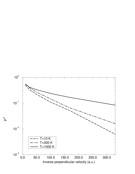
FIG. 2.: Final positive fractions versus the inverse of the velocity for four different temperatures: $T=10$, 300, 1000 K in the case $N=4$ and $U\rightarrow\infty$. The atom starts from equilibrium at $z_{0}=3$ a.u.

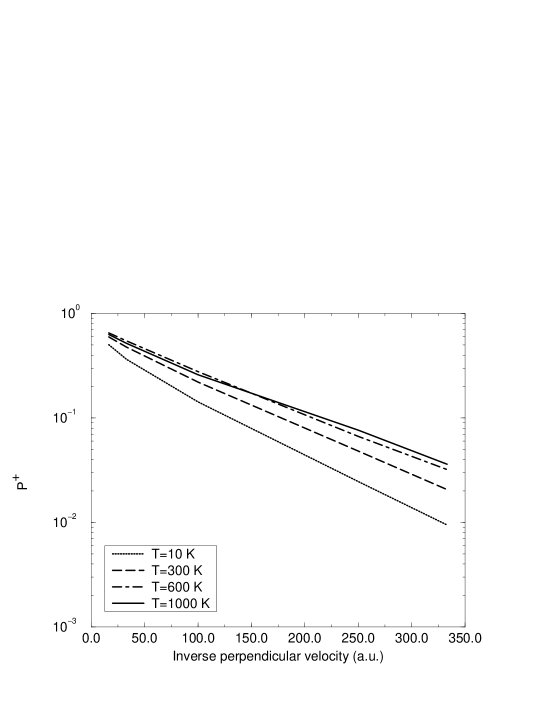
FIG. 3.: The same as in Fig. 2 but setting $N=2$.

As emphasized by SNL[6] the final fractions show strong temperature dependence which cannot be understood from an independent particle picture. Again setting $N=1$ the results of Fig. 4 show that the temperature dependence is in fact negligible as expected. There is some small temperature dependence at high temperatures, but this is just the usual thermal effect encountered previously in simple independent particle pictures[32].

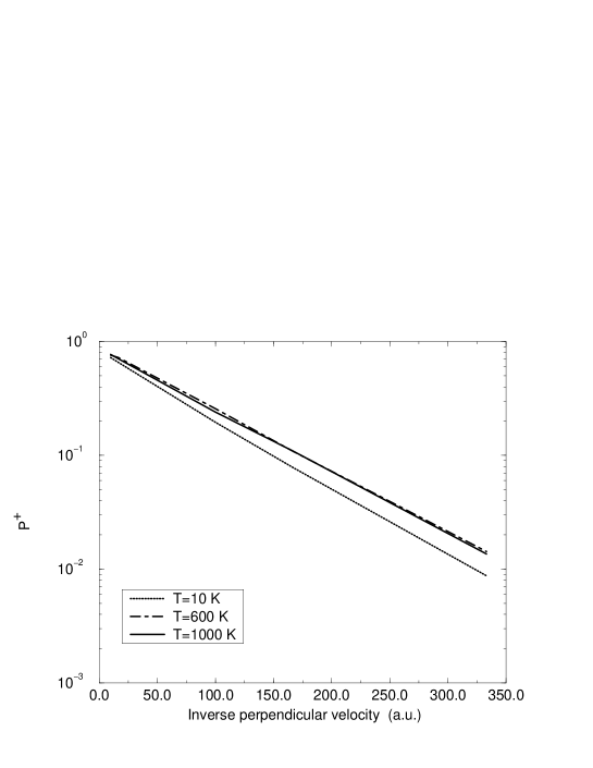
FIG. 4.: The same as in Fig. 2 but setting $N=1$.

In Fig. 5 we have also plotted the temperature dependence of the final fractions for four different degeneracies of the impurity: $N=1$, $2$, $4$ and $8$ and at a fixed velocity of $u_{f}=0.003$ a.u. While in the $N=1$ spinless case the final positive fractions remain fairly constant, for $N>1$ there is a strong temperature dependence of the final fractions with the temperature. As expected the temperature dependence is stronger for larger degeneracies of the atomic orbital.

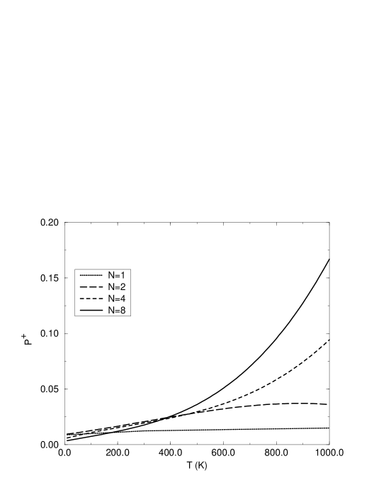
FIG. 5.: Final positive fractions versus temperature for a fixed velocity of $u_{f}=0.003$ a.u. and different degeneracies of the atom: $N=1$, 2, 4 and 8. The $U\rightarrow\infty$ limit has been taken, and the atom starts at $z_{0}=3$ a.u. in the equilibrium ground state.

Thus, as the temperature of the substrate decreases, neutralization takes place more efficiently. The effect may be understood from the static picture, as the screening of the unpaired spin of an impurity in a metal becomes more effective as the temperature drops below the Kondo scale. In the dynamical problem the final outgoing charge fractions reflect this fact as screening of both the unpaired spin and charge occur together.

Insight into the anomalous temperature dependence can be obtained by analyzing the renormalization of the parameters of the system when the atom is held at a fixed distance from the surface, at equilibrium. Table II records the values of the bare atomic level, the unrenormalized width, and Haldane’s scaling invariant[12], $E^{*}$, for different distances at zero temperature. Although perturbative scaling can only be safely applied in the weak coupling regime $\Delta_{a}\ll D$ and $U\gg D\gg|\epsilon_{a}|$, at sufficiently large distances from the surface (see Table) these conditions hold. The fraction $|E^{*}/\Delta_{a}|$ determines what regime the impurity is in. For most of the trajectory, the impurity is in the mixed-valence regime ($|E^{*}/\Delta_{a}|<1$). In this regime, $E^{*}$ can be identified as the renormalized level[1] and we see from Table II that the level is just above the Fermi energy in the relevant spatial region where the level width is sufficiently large to permit significant charge transfer. As the temperature is increased the renormalized level is thermally populated with holes from the metal enhancing the final positive fractions. For distances larger than $z=8.0$ a.u, the system reaches the empty orbital regime and the bare and renormalized energy levels converge as many-body effects are negligible. Of course in the spinless $N=1$ case, the level remains unrenormalized, and there is negligible temperature dependence in the final fractions[36].

TABLE II.: Haldane’s scaling invariant and renormalized levels for $N=2$. All energies are given in eV.

$z(a.u.)$	$\epsilon_{a}(z)$	$\Delta_{a}(z)$	$E^{*}(z)$	$E^{*}/\Delta_{a}$
$3.0$	$-2.4$	$2.90$	$-1.482$	$-0.510$
$4.0$	$-1.27$	$1.516$	$-0.474$	$-0.312$
$5.0$	$-0.7$	$0.7913$	$-0.122$	$-0.155$
$6.0$	$-0.36$	$0.4131$	$0.0267$	$0.0647$
$7.0$	$-0.13$	$0.2156$	$0.113$	$0.523$
$8.0$	$0.028$	$0.1126$	$0.180$	$1.602$
$9.0$	$0.150$	$0.0587$	$0.2412$	$4.104$
$10.0$	$0.244$	$0.03$	$0.30$	$9.722$

When the atom is sufficiently close to the surface it enters the local moment regime. If the atom stays for a long time in this situation, the electrons at the Fermi level couple antiferromagnetically with the unpaired spin of the atom and screen the impurity spin. An estimate of the Kondo temperature using the Bethe-ansatz[1] solution in the $U\rightarrow\infty$ at $z=3$ a.u. gives $k_{B}T_{K}\approx 0.1$ eV which approximately agrees with the position of the Kondo peak obtained from a plot of spectral density using the NCA approximation[36]. While in the spinless case the atomic level crosses the Fermi level when it approaches the surface, in the degenerate case $N>1$ the level sits just above it for a wide range of distances and eventually evolves into a Kondo resonance during the close encounter.

A simple estimate, within the independent particle picture, of the freezing distance $z_{fr}$ at which the charge transfer rate becomes small gives for $v=0.01$ a.u. the value $z_{fr}\approx 8$ a.u. This means that for perpendicular velocities $u_{f}\leq 0.01$ the empty orbital regime is always inside the freezing distance. This fact is corroborated in Fig. 1 as the charge fractions for $N>1$ converge to those of the independent particle picture at low enough perpendicular velocities and at zero temperature. However, for increasing surface temperature, as explained above, the renormalized level becomes populated. Analysis of the properties of this level via the spectral density led SNL[6] to conclude that the integrated charge under the Kondo peak actually freezes in the mixed valent regime, that is closer to the surface than what an independent particle picture suggests. This hypothesis explains why the anomalous temperature dependence persists even at very low velocities. Upon increasing the value of $N$ from 2 to 4 or 8, the energy renormalization increases further and the renormalized level lies above the Fermi level even for distances as close as $z=3$ to $4$ a.u.

In light of these results, it is interesting to reconsider how the Kondo effect might alter the phenomenon of loss of memory, the experimentally observed fact that the outgoing charge probability distribution of simple atoms such as alkalis and halogens does not depend on the incoming initial charge state. A stringent test of loss of memory is to study different initial conditions for the incoming ion: start the atom far away from the surface in a neutral and in a positive ion state. In Fig. 6 we see that both the neutral and positive yields are greater than the equilibrium ones. This breakdown of loss of memory for the case of the alkaline-earth atoms can be explained from the fact that the incoming atom creates particle-hole excitations in the metal which rise the temperature of the metal. In other words, the surface is heated locally by the formation of particle-hole pairs during the atom-surface interaction. Heating is greater in the case of the incoming positive ion as it induces a larger number of particle-hole pairs than an incoming neutral atom, because in both cases the atom emerges largely neutral. We find that an atom starting from equilibrium at $z_{0}=3$ a.u. with the surface at temperature $T=300$ K gives similar final fractions as those obtained for the positive ion scattered off of a zero-temperature surface.

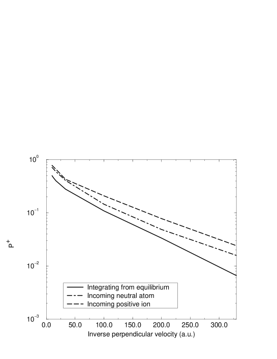
FIG. 6.: Different initial conditions: positive ion or neutral states starting from far away, with $u_{i}=u_{f}$, and the initial equilibrium ground state starting from $z_{0}=3$ a.u. The temperature $T=0$ K, $N=4$, and we have taken the $U\rightarrow\infty$ limit.

In contrast to the alkaline-earth atoms, we do not expect strong temperature dependence in the case of alkali atoms such as Li or Na. Close to the surface the atom is in the empty orbital regime, there is no unpaired spin to be screened, and there is no renormalization of the atomic level energy. Further out from the surface the local moment regime can occur, but the widths are too small for significant charge transfer to occur and the final fractions do not reflect any temperature dependence. Indeed, our calculations verify this picture, as shown in Fig. 7. Here the alkali atom has the same parameters as the alkaline-earth in the above calculations, with $N=4$ in the $U\rightarrow\infty$ limit. Only the nature of the atomic states has changed.

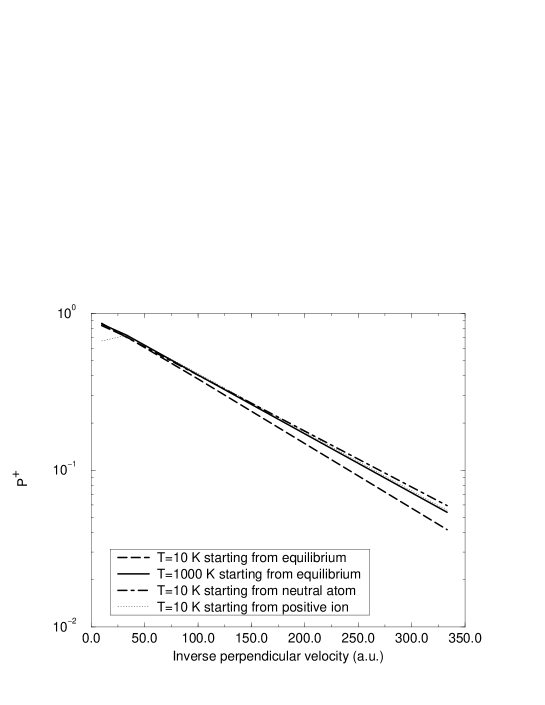
FIG. 7.: Temperature dependence with different initial conditions for the case of an alkali atom with the same parameters as used in Fig. 6.

It is reassuring to see that loss of memory is recovered in the alkali case and there is a negligible temperature dependence in the final occupancies.

B Finite U: Ca atoms bombarding Cu surfaces.

It was first suggested by SNL[6] that alkaline-earth atoms scattered off of noble metal surfaces are good experimental candidates to exhibit the anomalous temperature dependence. Ionization energies of alkaline-earth atoms are in the range of $4$ to $9$ eV, and work functions of noble metal surfaces range between $4$ and $5$ eV. The position of the atomic level with respect to the Fermi energy should not be greater than about $2$ eV; otherwise the yield of $AE^{+}$ ions is too small to be detected experimentally at the small velocities required. To be specific, we analyze in some detail the problem of calcium atoms scattering off copper surfaces. The experimental measured ionization energy of Ca is $6.1$ eV. The work function of the Cu(001) surface is $W=4.59$ eV. We now utilize a more realistic three parameter form for the widths to account for saturation at the chemisorption distance:

$${\Delta_{a}(z)}={{\Delta_{0}}\over{[{e^{4\alpha z}}{}~{}+~{}{{({\Delta_{0}}/{\Delta_{sat}})}^{4}~{}-~{}1~{}]}^{1/4}}}\ .$$ (25)

In all calculations that follow we take $\Delta_{0}=0.75$ a.u., $\Delta_{sat}=0.15$ a.u. and $\alpha=0.65$, both for the Ca${}^{0}(4s^{2})$ and for the Ca${}^{+}(4s^{1})$ levels. These parameters represent a “best guess” but it should be possible to obtain the parameters from first-principle, independent-particle calculations[26, 31].

We switch $N$ to its physical value, $N=2$, to model the actual spin degeneracy of the 4s level. The value of the $U$ is given by the difference between the first and second ionization levels. The energy required to remove an electron from the Ca⁺ 4s orbital is $11.9$ eV, so $U=5.8$ eV. We allow the level to vary in accord with the saturated form given in Sec. II, namely Eq.(13). We take the saturation of the first ionization energy of Ca to be $V_{maxI}=3$ eV. This choice is justified by recent DF-LCAO calculations which give the total energies of protons and He⁺ ions on Al metal[29, 31]. As discussed below, the qualitative behavior of our results do not depend on this choice. We also choose $V_{maxII}=3$ eV so that the second ionization energy of the Ca atom crosses the Fermi energy only for $z<3$ a.u. Although this choice may overestimate the production of Ca⁺⁺ close to the surface, it is a conservative condition to test the temperature dependence found above in the $U\rightarrow\infty$ limit. Recent trajectory simulations of Na atoms scattered from Cu surfaces in the hyperthermal energy range[35] suggest a turning point around $z_{0}=3$ a.u. is reasonable. In Fig. 8 we plot the final fractions as a function of the inverse of the perpendicular velocity.

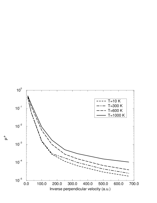
FIG. 8.: Final fractions versus inverse of the velocity for a Ca atom scattering from a Cu surface. The atom starts from the equilibrium ground state at $z_{0}=3$ a.u.

We have extended the calculations to perpendicular velocities as low as $u_{f}=0.0015$ a.u. We see that although the temperature dependence is somewhat reduced in comparison to the $U\rightarrow\infty$, the anomaly remains. The positive ion yield flattens out at low velocities, instead of decreasing rapidly, presumably because activity in the Ca⁺⁺ channel enhances the Ca⁺ fraction. This feature should be tested experimentally as it indirectly shows the role played by the virtual Ca⁺⁺ state. We have also tried doubling the total widths of the double hole-occupied state. The same temperature dependence is recovered.

In Fig. 9 we plot the evolution of the charge fractions along the trajectory of the ion for a fixed perpendicular velocity of $u_{f}=0.003$ a.u. From this figure we see that the Ca⁺⁺ recombines into Ca⁺ quickly due to the three times larger image shift in the second ionization energy as a function of distance, $3e^{2}/4(z-z_{im})$, compared to the first ionization level, which varies as $e^{2}/4(z-z_{im})$. This effect pushes the recombination of Ca⁺ ions into Ca⁰ out to further distances from the surface where the widths are not sufficiently large for complete neutralization of the positive fractions. This explains the enhancement in the probability of Ca⁺ ions seen in Fig. 8 for perpendicular velocities as small as $u_{f}=0.0015$ a.u. at $T=10$ K.

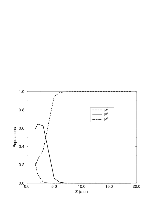
FIG. 9.: Evolution of the different charge fractions along the trajectory of a Ca atom starting from equilibrium at $z_{0}=3$ a.u. with surface temperature set to $T=10$ K

Finally we plot in Fig. 10 results for a Ca atom with the same parameters as those used previously in the limit $U\rightarrow\infty$. The Ca⁺ populations decay more quickly for $T=10$ K in the $U\rightarrow\infty$ limit than in the U-finite case. However, the $T=1000$ K plot in Fig. 10 resembles the $U=5.8$ eV case at zero temperature.

FIG. 10.: Final fractions for the same parameters as in Fig. 8 in the $U\rightarrow\infty$ limit.

For finite-$U$ Haldane’s scaling approach can be applied by replacing the half-bandwidth $D$ by $U$ in the renormalization group formulas[13]. For $U\approx D$ the position of the renormalized level and the scaling invariant do not change much from the $U\rightarrow\infty$ case for distances $z>5$ a.u. where perturbative scaling is justified.

Although an analytical expression for the Kondo temperature versus $U$ has been obtained [11] it is only valid to order O($1$) in the $1/N$ expansion. We do not expect it to give a realistic estimate of the Kondo scale for $N=2$. Quantum Monte Carlo calculations of spectral densities for the symmetric Anderson model suggest an increase in the Kondo temperature as the value of U is reduced[37]. In the asymmetric case, RG calculations have been carried out which give phenomenological expressions for the Kondo temperature. Unfortunately, the validity of these expressions is questionable for parameters appropriate to the atom-surface scattering problem.

In the above results we have only included the lowest energy Ca states: Ca${}^{0}(4s^{2})$, Ca${}^{+}(4s)$ and Ca${}^{++}(3p^{6})$. We now consider the effect of extending the atomic configurations to include the excited Ca${}^{+}(3p^{6}3d)$ state in the calculation. Its total energy is $7.8$ eV with respect to the neutral Ca${}^{0}(4s^{2})$ and therefore its ionization energy is $3.2$ eV measured with respect to the Fermi energy of a clean Cu(001) surface. We increase the decay exponent for this $3d$-state to $\alpha=1.00$ a.u. and keep the prefactor $\Delta_{0}$ and the saturation $\Delta_{sat}$ the same. Final fractions yield the same qualitative temperature dependence found above. The insensitivity of our result to the inclusion of this state suggests that the Kondo effect is robust.

IV Conclusions

We have shown that the Kondo screening cloud which surrounds an unpaired atomic spin reveals itself in an enhanced neutralization probability at low surface temperature. To demonstrate this we employed the dynamical $1/N$ expansion, extended to non-zero temperatures. The accuracy of the $1/N$ expansion was improved in comparison to previous work with the addition of a new sector at order O($1/N^{2}$). We calculated the final charge fractions of alkaline-earth atoms for different temperatures in the $U\rightarrow\infty$ limit, and found qualitative agreement with the NCA approach. We also analyzed the size of the temperature dependence for the case of degeneracies $N=1$, 2, 4, and 8. As expected, the anomalous temperature dependence is enhanced with increasing degeneracy of the atomic level. Furthermore, we performed a stringent test of the accuracy of the $1/N$ expansion by examining the spinless $N=1$ case. The Kondo effect disappears in this case, and also for alkali atoms, as it should.

A simple perturbative RG scaling argument explains the temperature dependence found in the degenerate cases. The bare atomic level is renormalized to just above the Fermi energy of the metal so that it can be thermally populated. Finally, we examined finite physical values of the Coulomb repulsion $U$ and excited states appropriate for real Ca atoms. Even though virtual Ca⁺⁺ ions are produced close to the surface, they rapidly recombine into Ca⁺ as the atom leaves the surface. Anomalously strong temperature dependence remains, although absolute yields differ somewhat from those obtained in the $U\rightarrow\infty$ limit.

Experimental detection of this effect may be possible, but several conditions must be satisfied. First, kinetic energy deposited in the lattice during the atom-surface impact must remain largely decoupled from the electronic degrees of freedom, otherwise the electrons in the surface will be heated and mask the Kondo effect. Furthermore, both the parallel and perpendicular components of the velocity must be kept small to avoid smearing the Fermi surface in the reference frame of the atom. Thus $k_{F}|\vec{u_{f}}|\ll k_{B}T$; for $T=1000$K this translates to $|\vec{u_{f}}|<0.004$ a.u. in the case of a Cu(001) surface. As final fractions smaller than $0.1\%$ are difficult to detect experimentally, it is important to choose the surface workfunction carefully. We considered the specific case of Ca hitting Cu(001), but yields can be increased by using different metallic surfaces with larger workfunctions. Finally, local heating of the surface in the form of particle-hole excitations produced as a by-product of charge transfer between the atom and the surface will mask the Kondo effect. Heating the surface, rather than cooling it, appears to be the best way to probe the anomalous temperature dependence, the cleanest signature of the Kondo effect.

Acknowledgements We thank Andone Lavery, Chad Sosolik, Eric Dahl, Barbara Cooper, Peter Nordlander and David Langreth for helpful discussions. Computational work in support of this research was performed on Cray computers at Brown University’s Theoretical Physics Computing Facility. J. Merino was supported by a NATO postdoctoral fellowship and JBM was supported in part by NSF Grant DMR-9313856.

REFERENCES

- [1] A. C. Hewson, The Kondo Problem to Heavy Fermions (Cambridge University Press, New York, 1993).
- [2] J. Kondo, Solid State Physics 23 (Academic Press, 1969).
- [3] K. G. Wilson, Rev. Mod. Phys. 47, 773 (1975).
- [4] A. J. Heeger, Solid State Physics 23, 283 (1975).
- [5] D. Goldhaber-Gordon, Hadas Shtrikman, D. Mahalu, D. Abusch-Magder, U. Meirav and M. A. Kastner, Nature 391, 156 (1998).
- [6] H. Shao, P. Nordlander and D. C. Langreth, Phys. Rev. Lett. 77, 948 (1996).
- [7] L. V. Keldysh, Soviet Phys. JETP 20 (1965) 1018; L. P. Kadanoff and G. Baym, Quantum Statistical Mechanics (Benjamin, New York, 1962).
- [8] H. Shao, D. C. Langreth, and P. Nordlander, Phys. Rev. B 49, 13929 (1994).
- [9] H. Shao, P. Nordlander and D. C. Langreth, Phys. Rev. B 52, 2988 (1995).
- [10] N. S. Wingreen and Y. Meir, Phys. Rev. B 49, 11040 (1994).
- [11] A. Schiller and V. Zevin, Phys. Rev. B 47, 9297 (1993).
- [12] F. D. M. Haldane, Phys. Rev. Lett. 40, 476 (1978).
- [13] H. R. Krishna-murthy, J. W. Wilkins and K. G. Wilson, Phys. Rev. B 21, 1003; Phys. Rev. B 21, 1044 (1980).
- [14] T. A. Costi, J. Kroha, P. Wölfe 53, 1850 (1996).
- [15] A. V. Onufriev and J. B. Marston, Phys. Rev. B 53, 13340 (1996).
- [16] J. B. Marston et al., Phys. Rev. B 48, 7809 (1993).
- [17] E. B. Dahl, E. R. Behringer, D. R. Andersson and B. H. Cooper, submitted to the Intl. J. Mass Spec. Ion. Proc.
- [18] D. M. Newns, Phys. Rev. 178, 1123 (1969).
- [19] R. Brako and D. M. Newns, Surf. Sci. 108, 253 (1981).
- [20] C. M. Varma and Y. Yafet, Phys. Rev. B 13, 2950 (1976).
- [21] O. Gunnarsson and K. Schönhammer, Phys. Rev. B 28, 4315 (1983).
- [22] O. Gunnarsson and K. Schönhammer, Phys. Rev. B 31, 4815 (1985).
- [23] R. Brako and D. M. Newns, Solid State Commun. 55, 633 (1985).
- [24] A. T. Amos, B. L. Burrows, and S. G. Davison, Surf. Sci. Lett. 277, L100 (1992); B. L. Burrows, A. T. Amos, Z. L. Miskovic, and S. G. Davison, Phys. Rev. B 51, 1409 (1995).
- [25] To obtain a copy of the computer program “alk.c” contact J. B. Marston.
- [26] P. Nordlander and J. C. Tully, Phys. Rev. Lett. 61, 990 (1988).
- [27] David Langreth, private communication.
- [28] P. Kurpick, U. Thumm, Phys. Rev. A 54, 1487 (1996).
- [29] J. Merino, N. Lorente, P.Pou, and F. Flores, Phys. Rev. B 54, 10959 (1996).
- [30] J. P. Gauyacq, A. G. Borisov, amd D. Teillet-Billy, in Negative Ions, edited by V. Esaulov (Cambridge University Press, Cambridge, 1993).
- [31] W. More, J. Merino, P. Pou, R. Monreal and F. Flores, Phys. Rev. B 58 7385 (1998).
- [32] J. Los and J. J. C. Geerlings, Phys. Rep. 190, 133 (1990).
- [33] D. C. Langreth, Phys. Rev. 150, 516 (1966).
- [34] N. E. Bickers, Rev. Mod. Phys. 59, 845 (1987).
- [35] C. A. DiRubio, R. L. McEachern, J. G. McLean and B. H. Cooper, Phys. Rev. B 54, 8862 (1996).
- [36] T. Brunner and D. C. Langreth 55, 2578 (1997).
- [37] J. Bǒnca and J. E. Gubernatis, 47, 13137 (1993).