THE QUANTUM MECHANICS OF CHAOTIC BILLIARDS

Abstract

We study the quantum behaviour of chaotic billiards which exhibit classically diffusive behaviour. In particular we consider the stadium billiard and discuss how the interplay between quantum localization and the rich structure of the classical phase space influences the quantum dynamics. The analysis of this model leads to new insight in the understanding of quantum properties of classically chaotic systems.

PACS number: 05.45.+b

I INTRODUCTION

When in a cold winter morning at the start of 1976 one of us (GC) entered the Institute of Nuclear Physics of the Siberian Division of the USSR Academy of Sciences in Akademgorodok, the main purpose was to discuss with the author Boris V. Chirikov, a startling paper which appeared as a CERN preprint at the end of the sixties[1]. Except to few, the paper remained almost unnoticed and practically none had the perception that this paper was a cornerstone of the new building of nonlinear science which, only few years later, expanded in an impressive way. Among other things, the so-called standard map or Chirikov map was discussed as a model of classical dynamical chaos. It was in that same occasion that we quantized the map thus obtaining the quantum kicked rotor which became later a basic model for the study of quantum chaos[2, 3].

The importance of the Chirikov map lies in the fact that it gives an approximate description of a wide class of dynamical systems. As a matter of fact it contains most of the complex features of dynamical motion. For these reasons its properties are continuously being studied and it is used in university courses to teach the emergence of random motion in deterministic systems.

In the quantum world the standard map played a fundamental role in bridging different fields of research: solid state physics, atomic physics, Random Matrix Theory. In particular it allowed to discover the phenomenon of quantum dynamical localization namely the fact that quantum interference effects suppress the classical diffusive process and lead to localization of the quantum excitation. This phenomenon had then been observed in several laboratory experiments in atomic physics[4, 5, 6, 7] and, more recently, a physical microscopic realization of the kicked rotator had been possible [8].

All the above experiments refer to systems under external perturbations. It was however not clear how quantum localization could take place in conservative systems. Indeed in this case an Eigenfucntion (EF) is always a superposition of a practically a finite number of unperturbed EFs and therefore it is not even clear what localization should mean here.

In Refs.[9, 10], by using a well known model of quantum conservative systems, the so-called WBRM model, it was shown that EFs can be localized inside the energy shell. More precisely, an ergodicity parameter $\lambda$ was introduced which acts as a scaling parameter. For $\lambda<1$ the EFs are localized inside the energy shell $\delta E$, while for $\lambda>1$ the EFs are extended or ergodic. The width $\delta E$ is the width ot the Local Density of States (LDOS) or strength function. Therefore for $\lambda>1$ an EF actually excites the maximum number of unperturbed states. As it is quite evident this problem calls in question the notion of quantum ergodicity [11].

It was then shown that quantum localization actually takes place in a more physical model of conservative systems: the billiard in a stadium [12]. The same effect was successively confirmed in a different shape, classically chaotic, billiard [13, 14].

The question remains open however, whether or not the mechanism of localization is the same as in WBRM. In particular it is necessary to understand how the structure of EF changes as one moves from the perturbative regime to the region of complete ergodicity.

In this paper, on the basis of the results of [15] , we discuss in detail the above problem. We show that contrary to WBRM, localization here manifests via the sparsity of the structure of the EFs and we surmise that this should be a general feature of localization in conservative systems. We also show that the presence of cantori in the classical motion plays an important role in the quantum motion. The “quantum cantori” should be observable in real laboratory experiments.

II THE CLASSICAL STADIUM BILLIARD

In this paper we mainly consider a stadium billiard, that is the motion of a free point particle of unit mass and velocity $\vec{v}$ (energy $E=v^{2}/2$) bouncing elastically inside a stadium-shaped well: two semicircles of radius $1$ connected by two straight line segments of length $2\epsilon$. The classical motion, for arbitrary small $\epsilon$, is ergodic, mixing and exponentially unstable with Lyapunov exponent $\Lambda\sim\epsilon^{1/2}$. It can be approximated (up to ${\cal O}(\epsilon)$) with the discontinuous stadium-map [12]

$$L_{n+1} = L_{n}-2\epsilon\sin\theta_{n}{\rm sgn}(\cos\theta_{n})\sqrt{1-L_{n}^{2}},$$ (1)

$$\theta_{n+1} = \theta_{n}+\pi-2\arcsin{L_{n+1}}\pmod{2\pi}$$ (2)

where $L=l/\sqrt{2E}$ is the rescaled angular momentum, $l=\vec{r}\wedge\vec{v}$, and $\theta$ is the polar angle (identical to the arc-length for small $\epsilon$). Note that, due to symmetry, the stadium map (1) has a period $\pi$ in the angle $\theta$. One should note also that the stadium map is topologically similar to the sawtooth map

$$p_{n+1} = p_{n}+K(x-\textstyle{\frac{1}{2}})$$ (3)

$$x_{n+1} = x_{n}+p_{n+1}\pmod{1}.$$ (4)

The behaviour of the sawtooth map (2) has been studied analytically and numerically in great detail [16, 17]. For the stadium billiard, due to the classical chaotic motion, the angular momentum $l$ undergoes, for small $\epsilon$, a process of diffusive behaviour

$$\langle(l_{n}-l_{0})^{2}\rangle\approx D(l_{0})n$$ (5)

with diffusion rate $D=D(l)$ which may depend on local value of angular momentum $l$. Rigorous results on the sawtooth-map [16, 17] have shown that the diffusion rate goes as $D\propto K^{5/2}$ if $K\ll 1$ or $D\propto K^{2}$ if $K\gg 1$. The same dependence $D\propto\epsilon^{5/2}$ on the small control parameter $\epsilon$ has been numerically found in [12] for the billiard and for the map (1). The factor $\sqrt{1-L_{n}^{2}}$ in the local shift of angular momentum leads to a dependence of diffusion rate on the local value of angular momentum. As a result, it is easily seen that, for the map (1):

$$D(l)=\gamma\epsilon^{5/2}(2E-l^{2}),$$ (6)

where the prefactor $\gamma\approx 2$ has been numerically computed. In figure 1 we show the weak dependence of $\gamma$ on the local angular momentum $l$ for various values of the parameter $\epsilon$ in the stadium billiard. Note that eq. (6) gives the diffusion rate in the discrete time $n$. The physical time $T$ between collisions depends on the local angular momentum, namely $T=\sqrt{2E-l^{2}}/E$. Since the stadium billiard is mixing, the classical dynamics will lead to the microcanonical equilibrium distribution. This implies that the equilibrium distribution of angular momenta is uniform in the discrete time

$$\rho_{\rm discr}(l)=1/\sqrt{8E}$$

(invariant measure of the approximate Poincaré map (1)) while, in the continuous time, it obeys the semicircle distribution

$$\rho(l)=\frac{1}{\pi E}\sqrt{2E-l^{2}}\propto T(l)\rho_{\rm discr}$$ (7)

(invariant measure of the smooth dynamics in the full phase space).

The power $5/2$ in eq. (6) (instead of $2$ as found for smooth deformations of the circle [13]), is due to the existence of cantori in the classical billiard motion which are also typical of discontinuous maps like (1,3) The cantori form strong obstacles to phase space transport and therefore they reduce the diffusion rate (even if the diffusion remains normal).

It is important to evaluate the flux ${\cal F}$ of the phase space area which is transported through a cantorus in one iteration of the map. For the sawtooth map there are no dominant cantori in phase space and the flux ${\cal F}$ is independent of the winding number of the resonance and is given by ${\cal F}=K^{2}/8\sqrt{D}$ where $D=K^{2}+4K$ [16].

Therefore, for small values of the control parameter $K$ the flux goes as $K^{3/2}$. We can now use this result to estimate the flux through cantori for the stadium map for small $\epsilon$. We obtain

$${\cal F}\approx(2E)^{1/2}\epsilon^{3/2}$$ (8)

which incorporates the correct energy scaling of phase space area.

The size of a cantorus ${\cal C}$, in the rescaled angular momentum variable $L$, that is $p_{\cal C}=\max_{\cal C}L-\min_{\cal C}L$, averaged over all the resonances, can be estimated from the exact results on sawtooth map [18]. After averaging over all the resonances one finds that the average size is proportional to the parameter $\epsilon$,

$$\bar{p}=c\epsilon,$$ (9)

where $c$ is some numerical constant. From our numerical computations on the stadium, $c$ turns out to be in the range $c=10$ for eps=0.05, and $c=15$ for eps =0.005. The fact that $c$ slowly increases with decreasing eps is due to existence of the cantorus along the separatrix of 2:1 resonance (around $L=0$) which has a larger size and scales as $p(2,1)\approx\sqrt{\epsilon}$. In figure 2a we illustrate the structure of cantori by showing a phase space portrait of a typical orbit ($\epsilon=0.003$) around the largest 2:1 resonance.

III THE QUANTUM DYNAMICS

In this section we consider the structure of quantum eigenfunctions for the stadium billiard $\Psi_{n}(\vec{r})$ which are solutions of the Helmholz equation

$$(\Delta\Psi_{n}+k_{n}^{2}\Psi_{n})=0.$$

with consecutive eigenenergies $E_{n}=k_{n}^{2}/2$. We consider only odd-odd states with Dirichlet boundary conditions on the quarter-stadium. It is interesting to consider the eigenstates $\Psi_{n}$ of the stadium billiard expressed in terms of eigenstates of the nearest integrable billiard, namely the circle billiard. The eigenfunctions of the unit quarter-circle billiard are

$$\Phi_{sm}(\vec{r})=J_{2s}(k^{0}_{sm}r)\sin(2s\phi),$$

where $k^{0}_{sm}$ are zeros of even-order Bessel functions. One may expand an eigenstate of the stadium billiard (for small $\epsilon$) in terms of eigenstates of a quarter-circle billiard

$$\Psi_{n}(\vec{r})=\sum_{sm}c^{n}_{sm}\Phi_{sm}(\vec{r})$$ (10)

The probability of having a value $l=2s$ of angular momentum (only even values of angular momentum are allowed due to symmetry) is

$$p_{n}(l=2s)=\sum_{m}|c^{n}_{sm}|^{2}.$$ (11)

If quantum eigenstates were ergodic one would expect to recover the classical microcanonical distribution (7) of angular momentum namely one would expect the quantum distribution

$$p_{n}(l=2s)\approx\rho(l)\propto\sqrt{2E_{n}-l^{2}}.$$ (12)

However, since the classical motion is approximated by the map (1), then in analogy with the quantization of the standard map, one would expect the phenomenon of quantum localization to take place with localization length $\ell$ proportional to the classical diffusion rate

$$\ell\sim D.$$ (13)

The localization length $\ell$, which is defined more precisely below (eq. (18), section 6), measures the (average) number of excited angular momentum eigenfunctions, that is the average width of the probability distribution $p_{n}(l)$.

In a bound conservative system like the stadium however, there are two main peculiarities which influence the process of quantum localization. First, the range of variation of angular momentum $l$ is finite, $-\sqrt{2E}\leq l\leq\sqrt{2E}$. As discussed in [12], this implies the existence of an upper bound for the localization length which is defined by the condition $\ell_{\max}=l_{\max}=\sqrt{2E}$. This leads, together with (13), to the delocalization or ergodicity border $\epsilon^{5}N\sim 1$, where $N\approx E/8=k^{2}/16$ is the sequential quantum number in the stadium billiard. Therefore, in order to observe ‘dynamical’ localization, this border must be above the perturbative border. The perturbative border is given simply by the condition $\epsilon\sqrt{2E}\sim 1$, which states that the length of the straight line segment of the stadium should be at least one de Broglie wavelength in order to be visible to quantum mechanics $\epsilon\sim(2E)^{-1/2}$. The same border can be obtained from the map (1) via the condition that in one iteration the change in angular momentum is at least one quantum $\Delta l\sim\epsilon\sqrt{2E}\sim 1$. Therefore, for small values of the parameter $\epsilon$ the two borders are well separated

$$N_{p}=\frac{1}{16}\epsilon^{-2}\ll N_{e}=\frac{1}{64}\epsilon^{-5},$$

and is possible to observe localization as actually done in [12].

The second peculiarity is due to the presence of cantori. Already long ago it has been surmised by McKay and Meiss [19] that cantori may act as perfect barriers for the quantum motion if the flux through cantori, for each iteration of the quantum map, is less than one Planck’s cell. However, to our knowledge, this effect has never been observed neither numerically nor experimentally and therefore it is not really known whether the above condition actually plays a role in quantum mechanics. For our present case of the stadium map this border can be estimated from the flux (8) ${\cal F}\sim x:=\epsilon^{3/2}\sqrt{2E}\sim 1$ (note that we have $\hbar=1$), and gives

$$N_{c}=\frac{1}{16}\epsilon^{-3}.$$ (14)

It is interesting to observe that, for sufficiently small $\epsilon$, this border is well separated from the other two borders $N_{p}\ll N_{c}\ll N_{e}$ and should be (numerically or experimentally) observable. Hence, for small values of the control parameter $\epsilon$, we expect to see four different regimes in the quantum dynamics of the stadium biliard: (1) perturbative regime for $N<N_{p}$, (2) pseudo-integrable or cantori regime where eigenstates are expected to be localized on classical cantori, for $N_{p}<N<N_{c}$, (3) dynamical localization for $N_{c}<N<N_{e}$, and finally (4) for sufficiently large energy, $N>N_{e}$, we should enter the regime of quantum ergodicity where (12) holds.

IV CANTORI AND QUANTUM MECHANICS

Here we would like to illustrate explicitly the effect of cantori on quantum eigenfunctions. In the regime where $x=\epsilon^{3/2}k<1$ it is natural to expect that cantori will influence the localization process. Indeed, as shown above, in such situation the cantori act as perfect barriers, and the quantum system looks as if classically integrable [20]. It is therefore expected that the localization length of eigenstates must be of the order of the size of cantori. On the other hand, since for small $\epsilon$ the cantori border can be much higher than the perturbative border, we may have here a nice possibility to study the effect of cantori in quantum mechanics. The average size of cantori has been found analytically and numerically to be (see section II, eq. (9))

$$\ell_{c}=c\epsilon l_{\max}=c\epsilon\sqrt{2E}$$ (15)

with $c$ a numerical constant. In figure 2b we show an eigenstate in angular momentum basis in the cantori region near the 2:1 resonance. In figure 3 (and also figure 4) our numerical data show that at $x=1$ the behaviour of localization length changes: for $x<1$ namely below the cantori border the localization length agrees with the theoretical estimate (15). This provides the first numerical evidence that the idea of flux quantization through cantori introduced in[19] is indeed correct. Even more convincing is the inspection of individual quantum eigenstates in the Husimi phase space representation (see figure 5) which show very clearly, that in the cantori region, the relative phase space area occupied by the localized eigenstates does not increase with increasing $\epsilon$ or with increasing $k=\sqrt{2E}$. We checked this even quantitatively, by computing the phase space area of Husimi phase space distributions via information entropy or inverse participation ratio [22]. The width of Husimi functions on quantized cantori in the perpendicular direction is given only by the width of the wavepacket which is used for the computation of Husimi functions (see section VI).

V INTERPLAY BETWEEN CANTORI AND DYNAMICAL LOCALIZATION

Above the quantum cantori border $x=1$ the flux through the turnstiles becomes larger than a Planck’s cell, the cantori do not act any more as barriers for quantum dynamics and the quantum motion starts to follow the classical diffusive behaviour up to the quantum relaxation time $t_{R}$ (break time), which is proportional to the density of operative eigenstates namely of those states which enter the initial condition and therefore actually control the quantum dynamics. For $t>t_{R}$ instead, the quantum dynamics enter an oscillatory regime around the stationary localized state. The density of operative eigenstates is by a factor $\ell/l_{\max}$ smaller than the total density of states

$$t_{R}=(\ell/l_{\max})dN/dE$$

and therefore the relaxation time is less than the Heisenberg time which is given by the level density. The angular momentum width $\ell$ of the localized state is then given by $\ell^{2}\approx Dt_{R}/T$, where $T\approx E^{-1/2}$ is the average time between bounces. This leads to the simple expression for the average (scaled) localization length

$$\ell/l_{\max}\approx D/k=\alpha\epsilon^{5/2}k$$ (16)

where $\alpha$ is a constant to be determined numerically. We need however to take into account the fact that for $x<1$ the width of eigenfunctions is determined by classical cantori and not by dynamical localization. Since we measure the localization length in angular momentum space, then for $x>1$, we need to add the average size of cantori to the angular momentum spread due to dynamical localization. Therefore, above the cantori border $x>1$, we expect the following expression for the numerical (scaled) localization length $\sigma_{n}=\ell_{n}/l_{\max}$,

$$\sigma_{n}=\bar{p}+(1-\bar{p})\alpha\epsilon(x-1)$$ (17)

which takes into account the fact that we need to rescale the total size of angular momentum space, and that for $x=1$, $\sigma_{n}=\bar{p}$ which is the average size of cantori as determined numerically. In figure 3 (see also figure 4) it is seen that expression (17) is in excellent agreement with our numerical data up to $N$ $\sim 10^{7}$ and for different values of $\epsilon$. The obtained value of the numerical constant is $\alpha=1.7$.

Notice that only for very small $\epsilon$ the constant contribution due to cantori in (17) will be negligible and localization length would be simply proportional to $D$, as given by eq. (16).

Notice also that due to the discontinuity of the stadium map, the quantum eigenfunctions are not exponentially localized, like for the standard map or for smooth chaotic billiards [13], but they have power-law tails

$$p(l)\propto|l-l_{0}|^{-4}$$

This is consistent with results based on the quantization of the stadium map [21], and with rigorous results on band random matrices with increasing band size [23]. In figure 6 we show two (averaged) localized states in angular momentum basis in which the power law tails are clearly seen.

The pseudo-integrable (cantori) regime may also be detected by inspecting the energy level statistics, e.g. the commonly studied nearest neighbour level spacing distribution $P(S)$, the delta3 statistics etc. As an example in figure 7 we show that $P(S)$ is nearly Poissonian in cantori regime while it is intermediate between Poisson and Wigner (GOE) in the regime of dynamical localization. We would like to stress that the above deviations from GOE predictions have no relation with periodic orbit theory and bouncing ball orbits.

VI LOCAL DENSITY OF STATES

The Hamiltonian $H$ of the stadium billiard may be written as a small deformation of the integrable circle billiard $H_{0}$, namely $H=H_{0}+\epsilon V$. The exact stadium-eigenstates may be expanded in terms of unperturbed quarter-cirlce eigenstates $\Phi_{sm}(\vec{r})$ where $k^{0}_{sm}$ are the eigenvalues of the integrable quarter-circle – the zeros of the even-order Bessel functions (10). Or, vice versa, we can express eigenstates of integrable quarter-circle in terms of exact eigenstates of the perturbed billiard by the same (orthogonal) matrix of coefficients $c^{n}_{sm}$,

$$\Phi_{sm}=\sum_{n}c^{n}_{sm}\Psi_{k_{n}}.$$

It is important to note that unlike for Wigner-band-random matrices [10] the matrix of coefficients $c^{n}_{sm}$, ordered with increasing wavenumber (energy), has been found to have a symmetric appearance (see figure 8a for an example). The structure of rows (expansions of exact states in terms of circle states) is very similar to the structure of columns (expansions of circle states in terms of exact states). The effective bandwidth $b$ of the matrix $c^{n}_{sm}$ determines the width of the energy shell $\delta E=b$ while the effective number of nonzero entries in each row (fixed $n$) is proportional to the localization length $\ell$ of that state $\Psi_{n}$. Such a symmetry between perturbed and unperturbed states seems to be generic for conservative Hamiltonian systems. Indeed, a similar structure of the matrix of coefficients has been found for the chaotic rough billiards (with shapes of wiggled circles) introduced in [13] as well. However, the bandwidth $b$ for the stadium billiard has been found to take always its maximal value, that is

$$b\approx l_{\rm max}=\sqrt{2E},$$

independent of the parameter $\epsilon$, except in the perturbative regime $N<N_{p}$ where it becomes smaller. This should be contrasted with chaotic rough billiards [13] for which, below the so called Wigner-ergodicity border, the bandwidth $b$ has been found to decrease as $b\approx\epsilon^{2}N$.

Below the ergodicity border, $N<N_{e}$, $\ell<l_{\max}$, the matrix $c^{n}_{ms}$ is sparse in both horizontal and vertical directions (see figure 8a). (Note that the same is true also for the rough billiard) As a consequence of that, the averaged local density of states (LDOS),

$$w(k)=\langle\sum_{n}|c^{n}_{sm}|^{2}\delta(k+k^{0}_{sm}-k_{n})\rangle_{sm}$$

(averaged columns shifted to the same center) is nearly the same as average EF in circular basis

$$W(k)=\langle\sum_{sm}|c^{n}_{sm}|^{2}\delta(k+k_{n}-\langle n|\sqrt{2H_{0}}|n\rangle)\rangle_{n}$$

(average rows shifted to the same mean). See figure 8b. Both distributions, $W(k)$ and $w(k)$, agree quite well with the theoretical distribution $W_{e}(k)=(\sin(k)/k)^{2}/\pi$ which has been proposed[13] for LDOS of nearly circular billiards in the regime of quantum (Shnirelman) ergodicity.

Such structure is found in the regime of dynamical localization as well as in the regime of cantori localization where the quantum system behaves as if classically integrable. We would like to stress that for the case of WBRM there is instead a strong asymmetry in the sense that the EF’s are solid and narrow, namely they are localized inside the energy shell, while the expansion of a basis state in terms of exact EF’s shows a sparse structure [10].

VII NUMERICAL METHODS

A Computation of eigenstates of quantum stadium billiard

In order to check the above theoretical predictions we had to compute numerically the quantum eigenfunctions $\Psi_{n}(\vec{r})=\Psi_{k_{n}}$ of chaotic billiards which are solutions of the Schrödinger equation $(\Delta+k^{2}_{n})\Psi_{n}=0$ (where $\hbar=1$) satisfying Dirichlet boundary conditions along the boundary. We had to compute eigenstates with extremely large sequential quantum numbers $N$ of the desymmetrized stadium billiard (and also of the rough billiards) up to $N\approx 10^{7}$.

We have used a recently proposed scaling method [24], but we expanded quantum eigenfunctions $\Psi_{k}(\vec{r})$ in terms of more suitable circular waves (here we consider only odd-odd states)

$$\Psi_{k}(\vec{r})=\sum_{s=1}^{M}a_{s}J_{2s}(kr)\sin(2s\theta)$$

instead of the originally proposed plane waves. The eigenvalue $k=\sqrt{2E}$ is determined by minimizing a certain positive bilinear form along the boundary of the billiard [24]. This can be done by solving a generalized eigenvalue problem of dimension $\approx k$ which yields $\sim 10\%k$ accurate eigenvalues $k_{n}$ and eigenvectors $a^{n}_{s}$ simultaneously. Therefore, with this method, the computer workload required per energy level is by a factor $k$ or even $10k$ (namely from $10^{3}$ to $10^{4}$ for $k=10^{3}$) smaller than with more traditional methods, like the original Heller’s plane wave decomposition or boundary integral method!

B Definition and computation of localization length

Note that the magnitude of coefficients $a^{n}_{s}$ is proportional to the probability (11) of having angular momentum $l=2s$ in a quantum state $\Psi_{n}$,

$$p_{n}(l=2s)=|a_{s}|^{2}\int_{0}^{1}drr|J_{2s}(kr)|^{2}\propto|a_{s}|^{2}\sqrt{1-l^{2}/k^{2}}.$$

The number of levels below a given wavenumber $k$ or energy $E$, in a desymmetrized billiard, is given by the Weyl formula $N=k^{2}/16=E/8$.

The effective spread in angular momentum of an eigenstates $\Psi$ is characterized by the localization length $\ell$ which measures the typical number of $p_{n}(l)$ values which are substantially different from zero, or the size of the angular momentum interval in which $p(l)$ is significantly different than zero. Of course, there is no a unique definition of localization length. In particular the choice is quite delicate for the quantum stadium where localization is algebraic unlike billiards with smooth boundary where localization is expected to be exponential. We have therefore considered four different working definitions: (i) spread in angular momentum

$$\ell_{1}=\beta_{1}(\langle\Psi|\hat{l}^{2}|\Psi\rangle-\langle\Psi|\hat{l}|\Psi\rangle^{2})^{1/2},$$

(ii) information entropy

$$\ell_{2}=\beta_{2}\exp\left(-\sum_{l}p(l)\ln p(l)\right)$$

(iii) inverse participation ratio,

$$\ell_{3}=\beta_{3}(\sum_{l}[p(l)]^{2})^{-1},$$

(iv) $99\%$ probability localization length

$$\ell_{4}=\beta_{4}\min\{\#{\cal A};\sum_{l\in{\cal A}}p_{k}(l)\geq 0.99\}.$$ (18)

The numerical constants $\beta_{j},j=1,2,3,4$ have been determined with the condition that $\ell_{j}$ should take the maximal value $l_{\max}=k=\sqrt{2E}$ in the regime of quantum ergodicity. All the four definitions of localization length give qualitatively the same results. However, the $99\%$ localization length (18) which is proportional to the minimal number of angular momentum eigenvalues that are needed to support $99\%$ probability, is the least sensitive to the slowly (algebraically) decaying tails of the distribution $p(l)$ and has given the sharpest and less fluctuating numerical results. The results shown in figures $3$ and $4$ were obtained using the definition (18) of localization length with the numerical value$\beta_{4}=1.38$.

C Computation of Husimi functions

In figure 5 we show Husimi functions of (quarter) stadium eigenstates on the Poincaré-Birhkoff section, with coordinates $(\varphi,l)$. The desymmetrized phase space is a rectangle $(\varphi,l)\in[0,\pi/2]\times[0,k],k=\sqrt{2E}$. We consider (almost) minimal wavepackets $|l\theta\rangle$ at phase space point $(\theta,l)$, which in the angle representation $|\varphi\rangle$, $0\leq\varphi<2\pi$ read

$$\langle\varphi|\theta,l\rangle=C\exp\left(-\frac{2a}{k}\sin^{2}(\textstyle{\frac{1}{2}}(\varphi-\theta))+il\varphi\right)$$ (19)

where $C$ is a normalization constant and $a$ is the aspect ratio. We take $a=1$ which means that the wavepacket has the same relative size in both directions. The Husimi function $h(\varphi,l)$ of a billiard eigenstate $\Psi(\vec{r})$ is computed w.r.t. the normal derivative of an eigenfunction along the boundary $\vec{r}(\varphi)$, $\partial_{n}\Psi=(d\vec{r}/d\varphi)\wedge\nabla\Psi/||d\vec{r}/d\varphi||$,

$$h(\theta,l)=|\int d\phi\langle\phi|\theta,l\rangle\partial_{n}\Psi(\vec{r}(\phi))|^{2},$$ (20)

where the numerical integration along the boundary of the billiard has been performed accurately using high-order Gaussian quadratures.

VIII CONCLUSIONS

The billiard in a stadium is a very clean mathematical model of classical chaos and it is therefore particularly convenient to study the modifications that quantum mechanics introduces in our general picture of deterministic chaos. While the classical motion is ergodic and mixing for any non zero values of the parameter $\epsilon$, the quantum motion, as we have seen in this paper, exhibits a very rich structure and different regimes of motion as a function of the parameter $\epsilon$ or the energy $E$. Two are the main points we would like to stress: a) classical cantori may have strong effects on quantum mechanics. They lead to a new quantum border which is distinct from the perturbative border and from the localization border. In the regime of quantum cantori the rescaled localization length $\ell/k$ does not depend on energy or wavenumber $k$. In other words, the quantum dynamics is basically determined by the classical structure. This effect should be observable in real experiments. b) The mechanism of localization is strictly connected to the sparsity of EF’s when expanded on the basis of unperturbed circle states (or vice versa, sparsity of unperturbed states when expanded in terms of the stadium EF’s). When we increase perturbation (or decrease $\hbar$), sparsity decreases, localization length of EF’s increases until the delocalized or quantum ergodic regime is reached. We conjecture that this mechanism of localization is typical of conservative Hamiltonian systems. Quite interestingly, the mechanism of localization in WBRM is quite different and is associated to an asymmetry between EF’s (solid and narrow) and unperturbed states (delocalized but sparse). In this sense, WBRM cannot be taken to represent the typical behaviour of classically chaotic conservative systems.

The main impulse to the present paper originated from a previous work of B.Chirikov[25] in which a wiggled circle billiard was introduced as a model for localization in conservative systems. Also we have benefit from several results on the standard map. This confirms the importance and generality of the Chirikov standard map for the study of classical and quantum deterministic chaotic motion. Since 30 years, generations of physicists all around the world, have learned the beauty and complexity of nonlinear dynamics on the base of this apparently simple map. We believe that the Chirikov map is at the root of the impressive growth of the whole field of nonlinear dynamics and chaos. Strangely enough this fundamental contribution of B.V. Chirikov to one of the main achievements of physics of this century has never been properly recognized. Several years ago, in a friendly private letter to a colleague concerning a paper in which he failed to give the necessary credit to Chirikov, a common friend Joseph Ford, now deceased, wrote ”..why not give to the old Russian bear his due?”. We would like to turn this question to the scientific community. One of the authors of the present paper(GC), would like to take the opportunity of this special issue of the journal to express his deep gratitude to his friend and teacher Boris Valerianovich Chirikov.

Figure caption

FIG. 1.: The rescaled classical diffusion rate (4) $D(l)/[\epsilon^{5/2}(2E-l^{2})]$ as a function of the local value $L=l/\sqrt{2E}$ of the angular momentum for different values of the control parameter $\epsilon$.

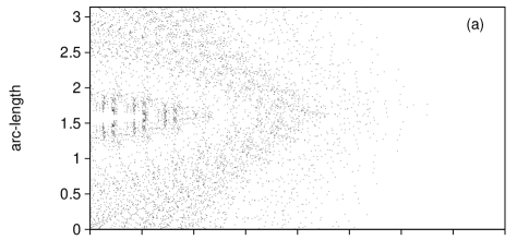
FIG. 2.: Time evolution of a single classical orbit, followed up to $20,000$ bounces, for the classical billiard with $\epsilon=0.003$. The orbit is initially started in the middle of the largest ‘island’ ( $L=0,\theta=\pi/4-0.0016$) (fig 2a). Angular momentum probability distribution $p(l)$ of the corresponding eigenstate with $\epsilon=0.003$ and eigenvalue $k=5999.8166$. As it is seen the state is uniformly distributed over the cantorus in the main island (Fig.2b). Notice also the same eigenstate in Husimi phase-space representation (2nd state in Fig.5b).

FIG. 3.: Rescaled localization length $\sigma=\ell/k$ versus the scaling variable $x=\epsilon^{3/2}k$ for five different values of $\epsilon$ ($60<k<12,000$). Each point is obtained by averaging over a large number $\nu$ of consecutive eigenstates ($\nu=100$ for small $k$ and $\nu=1,000$ for large $k$). The numerical data clearly show the cantori border $x=1$. In the cantori region $\ell/k$ is constant as expected, while for $x>1$ the numerical data agree with the theoretical prediction (17)(dotted curves). For large $x$, the value of localization length $\sigma$ approaches the maximal ergodic value $\sigma=1$.

FIG. 4.: Rescaled localization length $\sigma$ versus $\epsilon$ for two different wavenumbers $k$. The full lines give the classical estimate for the average width of cantori. It is seen that below the cantori border $x=1$($\epsilon=0.003$ for $k=6,000$ and $\epsilon=0.0063$ for $k=2,000$) the localization length is proportional to $\epsilon$ and independent on $k$. Above the border $x=1$ instead, the numerical data follow the analytical estimate (15) (dotted curves).

Color figure 5 (a-d) in (Windows/OS2 bitmap format) can be obtained by e-mail request on prosen@fiz.uni-lj.si

FIG. 5.: The Husimi phase space representation of quantum eigenstates of the stadium for different values of parameters $\epsilon$ and $k=\sqrt{2E}$. The Husimi function of a normal derivative of an eigenfunction along the boundary of desymmetrized (quarter) stadium billiard (section VII) is plotted (x-axes: angle $0\leq\varphi\leq\pi/2$, y-axes: angular momentum $0<l<\sqrt{2E}$). We show four consecutive eigenstates in the following order: up-left, up-right, down-left, down-right for (a) $\epsilon=0.001$, $k=5999.9775$, $5999.9812$, $5999.9815$, $5999.9818$, $(N\approx 2.25\cdot 10^{6})$, (b) $\epsilon=0.003$, $k=5999.8138$, $5999.8166$, $5999.8165$, $5999.8175$, (c) $\epsilon=0.01$, $k=6000.0079$, $6000.0104$, $6000.0112$, $6000.0121$, and (d) $\epsilon=0.01$, $k=12000.0030$, $12000.0040$, $12000.0041$, $12000.0051$, $(N\approx 9\cdot 10^{6})$. Note that the second state in (b) is the same as in figure 2b. The color scale (to the right of each figure) is proportional to the logarithm of Husimi function (white is large, black is small, entire color scale extends over 8 orders of magnitude, a factor of $10^{8}$. The cases (a,b) are in cantori region and one should note that the sizes of bright regions are roughly the same, while (c,d) are in the region of dynamical localization.

FIG. 6.: Average shape of eigenstates in angular momentum representation. (before averaging all the eigenstates have been shifted to the same mean value $\langle l\rangle$ of angular momentum. The average has been made over about thousand consecutive eigenstates for $\epsilon=0.005,k\approx 12000$ (regime of dynamical localization), and $\epsilon=0.001,k\approx 6000$ (cantori regime). The dotted lines give the expected slope $-4$ for the tails.

FIG. 7.: The nearest neighbour energy level spacing distribution $P(S)$. We show data for the two spectral stretches in the same energy window, $1993.8\leq k\leq 2006.2$ ($N\approx 250,000$), containing about $3,100$ levels each, namely $\epsilon=0.002$ (cantori region), and $\epsilon=0.02$ (region of dynamical localization). The theoretical Poisson and Wigner statistics are shown for comparison. Notice that in the cantori region $\epsilon=0.002$ (much above the perturbative border) the numerical data closely follow the Poissonian statistics (the deviation is only slightly larger than the expected statistical error).

FIG. 8.: The structure of the matrix of coefficients $c^{n}_{sm}$ in the regime of dynamical localization: $\epsilon=0.01$, $k\approx k_{0}:=2000.0$ (Fig.8a) A small dot at abscissa $k^{0}_{sm}-k_{0}$ and ordinate $k_{n}-k_{0}$ is plotted if $|c^{n}_{sm}|^{2}>0.02$ and a large dot if $|c^{n}_{sm}|^{2}>0.1$. Notice that the total number of levels along each axis is about 1250. In Fig.8b we plot the average local density of states $w(k-k_{0})$ and the average eigenfunction $W(k-k_{0})$ for the same $\epsilon=0.01$, averaged over a stretch of $5000$ consecutive eigenstates in the interval $1990<k<2010$. The dotted curve gives the theoretical LDOS for an ergodic billiard $W_{e}(k)=(\sin(k)/k)^{2}/\pi.$

REFERENCES

- [1] B.V. Chirikov, Investigation of the Theory of Nonlinear Resonance and Stochasticity, preprint Novosibirsk INP 267,1969.(CERN translation 71-40, Geneva, 1971).
- [2] G.Casati, B.V.Chirikov, J.Ford and F.M Izrailev, Lecture Notes in Physics 93, 334 (1979)
- [3] G.Casati and B.V.Chirikov, eds., Quantum Chaos: Between Order and Disorder, Cambridge University Press (1994); Physica D86, 220 (1995).
- [4] G.Casati, B.V.Chirikov, I.Guarneri and D.L.Shepelyansky, Phys. Rep. 154, 77 (1987); G.Casati, I.Guarneri and D.L.Shepelyansky, IEEE J. of Quantum Electr. 24, 1420 (1988).
- [5] J.E. Bayfield, G. Casati, I. Guarneri and D.W. Sokol, Phys. Rev. Lett. 63 (1989) 364.
- [6] E.J. Galvez, B.E. Sauer, L. Moorman, P.M. Koch and D. Richards, Phys. Rev. Lett.61 (1988) 2011.
- [7] M. Arndt, A. Buchleitner, R.N. Mantegna and H. Walther, Phys. Rev. Lett. 67 (1991) 2435.
- [8] F.L. Moore, J.C. Robinson, C. F.Bharucha, B. Sundaram, and M.G. Raizen Phys. Rev. Lett. 75, 4598(1995).
- [9] G. Casati, B.V. Chirikov, I. Guarneri and F.M. Izrailev, Phys. Rev. E 48, R1613 (1993).
- [10] G. Casati, B.V. Chirikov, I. Guarneri and F.M. Izrailev, Physics Letters A223 (1996) 430.
- [11] G. Casati,”On the foundation of equilibrium quantum statistical mechanics”. Preprint, cond-mat/9801063
- [12] F.Borgonovi, G.Casati and B.Li, Phys. Rev. Lett. 77, 4744 (1996).
- [13] K.Frahm and D.Shepelyansky, Phys.Rev.Lett. 78, 1440 (1997); ibid. 79, 1833 (1997).
- [14] K.Frahm, Phys.Rev.B, 55, 8626 (1997)
- [15] G.Casati and T.Prosen,”quantum localization and cantori in chaotic billiards”, submitted to phys. rev. lett. preprint, cond-mat/9704084.
- [16] Q.Chen, I.Dana, J.D.Meiss, N.W.Murray, and I.C.Percival, Physica D 46, 217 (1990).
- [17] I.Dana, N.W.Murray, and I.C.Percival, Phys.Rev.Lett 62, 233 (1989).
- [18] Average the expression for , pp225, weigted by phase-space areas of resonances (eq.33) of [16].
- [19] R.S. MacKay and J.D. Meiss, Phys. Rev. A37 (1988) 4702.
- [20] This integrable-like behaviour maybe at the root of the analytical results in: R.E. Prange and R. Naverich”Quasiclassical surface of section perturbation theory”. Preprint.
- [21] F. Borgonovi, ”Localization in discontinuous quantum systems” Preprint, chao-dyn/9801032
- [22] T.Prosen, Physica D91, 244 (1996).
- [23] A.D.Mirlin, Y.V.Fyodorov, F.-M. Dittes, J. Quezada, and T.H.Seligman, Phys.Rev.E 54 3221.
- [24] E.Vergini and M.Saraceno, Phys.Rev.E 52, 2204 (1995).
- [25] B.V. Chirikov, Linear chaos, preprint Novosibirsk INP 90-116