Quantum invariants of motion in a generic many-body system

Abstract

Dynamical Lie-algebraic method for the construction of local quantum invariants of motion in non-integrable many-body systems is proposed and applied to a simple but generic toy model, namely an infinite kicked $t-V$ chain of spinless fermions. Transition from integrable via pseudo-integrable (intermediate) to quantum ergodic (quantum mixing) regime in parameter space is investigated. Dynamical phase transition between ergodic and intermediate (neither ergodic nor completely integrable) regime in thermodynamic limit is proposed. Existence or non-existence of local conservation laws corresponds to intermediate or ergodic regime, respectively. The computation of time-correlation functions of typical observables by means of local conservation laws is found fully consistent with direct calculations on finite systems.

PACS numbers: 03.65.Fd, 05.30.Fk, 05.45.+b

We investigate the existence of Local Quantum Invariants of motion (LQI) (i.e. conservation laws) in a generic quantum many-body system of interacting particles. For sufficiently strong non-linear coupling between particles one expects quantum mixing and quantum ergodicity [1] which is incompatible with existence of LQI [2]. In this regime (hereafter referred to as quantum ergodic), time-correlations between arbitrary pair of quantum observables decay to zero. This property of quantum ergodicity is absolutely necessary for the derivation of the laws of normal transport within linear response theory. In another extreme case of completely integrable quantum many-body systems, an infinite number of LQI exist, and such systems are manifestly non-ergodic. Anomalous (ideal) transport properties of completely integrable quantum many body systems have been discussed in [3]. Our hypothesis is that generic non-integrable quantum many-body system of (locally) interacting particles may not be quantum ergodic, not even in thermodynamic limit (TL) (size $\rightarrow\infty$ and fixed density), provided that the system is sufficiently close to some completely integrable point in the parameter space (analogy with order to chaos transition of classical systems of few interacting particles). In a recent work [4] we conjectured and demonstrated the existence of intermediate, neither completely integrable nor ergodic, dynamical regime of a generic non-integrable quantum many-body system in TL, by directly inspecting its time evolution. It is the purpose of this paper to show that such an intermediate regime may be characterized by quantum pseudo-integrability: existence of at least one or few LQI, which is a sufficient condition, using a relation proposed by Mazur [5] and Suzuki [6], to prevent time correlations of certain observables to decay to zero.

In [4] a novel family of simple but generic many-body systems of locally interacting particles has been introduced smoothly interpolating between integrable and ergodic regime, namely kicked t-V model (KtV) of spinless fermions with periodically switched nearest neighbor interaction on an infinite chain with time-dependent Hamiltonian

$$H(\tau)=\sum_{j}\left[-\textstyle{\frac{1}{2}}t(c^{\dagger}_{j}c_{j+1}+h.c.)+\delta_{p}(\tau)Vn_{j}n_{j+1}\right],$$ (1)

$c_{j}^{\dagger},c_{j},n_{j}=c^{\dagger}_{j}c_{j}$ are fermionic creation, annihilation and number operators, respectively, and $\delta_{p}(\tau)=\sum_{m=-\infty}^{\infty}\delta(\tau-m)$. The time-dependent Hamiltonian (1) can be written as $H(\tau)=tH_{1}+\delta_{p}(\tau)VH_{0}$ where the dimensionless kinetic energy $H_{1}$ and the kick potential $H_{0}$ may be rewritten in terms of independent spin variables $(\sigma^{\pm}_{j},\sigma^{z}_{j})$ on sites $j$, via Wigner-Jordan transformation,

$$H_{1}=\textstyle{\frac{1}{2}}\sum_{j}(\sigma^{+}_{j}\sigma^{-}_{j+1}+\sigma^{-}_{j}\sigma^{+}_{j+1}),\quad H_{0}=\textstyle{\frac{1}{2}}\sum_{j}\sigma^{z}_{j}\sigma^{z}_{j+1}.$$

Symmetric time evolution of KtV system for one period is given by explicit unitary quantum many-body map ($\hbar=1$), $U=\hat{T}\exp(-i\int_{-1/2}^{1/2}d\tau H(\tau))=\exp(-itH_{1}/2)\exp(-iVH_{0})\exp(-itH_{1}/2).$ Note that $V$ is a cyclic parameter of period $2\pi$, and the dynamics is essentially invariant w.r.t. transformations $t\rightarrow-t$ and $V\rightarrow-V$, so we consider only the half-strip $(t,V)\in[0,\infty)\times[0,\pi)$. KtV model is completely integrable for: $t=0$ (Ising model), or $V=0\pmod{2\pi}$ (free fermion model), or $t,V\rightarrow 0$ and $t/V$ finite (XXZ model).

We prefer to consider Heiseberg representation and write a map over the algebra $\mathfrak{U}$ of quantum observables $A(\tau)$ for time evolution over one period, ${\hat{U}}_{{\rm ad\,}}:A(n-\textstyle{\frac{1}{2}})\rightarrow A(n+\textstyle{\frac{1}{2}})=U^{\dagger}A(n-\textstyle{\frac{1}{2}})U$, explicitly as

$${\hat{U}}_{{\rm ad\,}}=\exp\left(\frac{it}{2}{\rm ad\,}H_{1}\right)\exp\left(iV{\rm ad\,}H_{0}\right)\exp\left(\frac{it}{2}{\rm ad\,}H_{1}\right).$$

where ${\rm ad\,}$ is the usual adjoint map on the Lie algebra $\mathfrak{U}$, ${\rm ad\,}A:B\rightarrow[A,B]=AB-BA$. Infinite-dimensional Lie algebra $\mathfrak{U}$ of local quantum observables is also a Hilbert space equiped with the invariant bilinear form

$$(A|B)=\lim_{L\rightarrow\infty}\frac{1}{L2^{L}}{\rm tr}_{L}A^{\dagger}B$$ (2)

which is a scalar product invariant under the adjoint map ${\rm ad\,}A:B\rightarrow[A,B]$, $(({\rm ad\,}A^{\dagger})B|C)=(B|({\rm ad\,}A)C)$. The limit and the trace ${\rm tr}_{L}$ is defined thru finite systems of increasing size $L$. Our aim is to check the existence of LQI which are the (normalizable [7]) fixed points $A$ ($(A|A)<\infty$) of the Heissenberg map ${\hat{U}}_{\rm ad\,}$

$${\hat{U}}_{{\rm ad\,}}A=A.$$ (3)

However, we do not suggest to solve eq. (3) in the full algebra $\mathfrak{U}$ which is a highly prohibitive task. Instead, we devise a special subalgebra of $\mathfrak{U}$, the Minimal Invariant Lie Algebra (MILA), which is invariant to motions generated by the kinetic or the potential part of the Hamiltonian and hence it is also invariant to $U_{{\rm ad\,}}$. Having the two generators, $H_{0}$ and $H_{1}$, spanning 2-dim subspace ${\mathfrak{s}}=\{\alpha H_{0}+\beta H_{1}\}$, we construct the basis of MILA ${\mathfrak{S}}=\bigcup_{n=1}^{\infty}({\rm ad\,}{\mathfrak{s}})^{n}{\mathfrak{s}}$ ordered by the order of locality as follows: We assign an observable $\tilde{H}_{p,b}$ to an ordered pair of integers $(p,b)$, order $p$, and code $b,\,0\leq b<2^{p}$ with $p$ binary digits $b_{n},\,b=\sum_{n=0}^{p-1}b_{n}2^{n}$, namely

$$\tilde{H}_{p,b}=({\rm ad\,}H_{b_{p-1}})({\rm ad\,}H_{b_{p-2}})\cdots({\rm ad\,}H_{b_{1}})H_{b_{0}}.$$

Since not all observables $\tilde{H}_{p,b}$ upto a given maximal order $q,p\leq q,$ are linearly independent we perform Gram-Schmit orthogonalization w.r.t. the scalar product (2)

$$G_{q,c} = \cases{\tilde{G}_{q,c}/\sqrt{(\tilde{G}_{q,c}|\tilde{G}_{q,c})};&$\tilde{G}_{q,c}\neq 0$,\cr 0;&$\tilde{G}_{q,c}=0$,\cr}$$ (4)

$$\tilde{G}_{q,c} = \tilde{H}_{q,c}-\sum_{(p,b)}^{(p,b)<(q,c)}G_{p,b}(G_{p,b}|\tilde{H}_{q,c}).$$ (5)

The nonzero (normalized) local observables $G_{q,c}$ form the orthonormal basis of MILA. Note that observables $G_{q,c}$ are local operators of order $q$, they have been expanded in terms of spatially homogeneous finite products of field operators, say $Z_{s_{0}s_{1}\ldots s_{q}}=\sum_{j}\sigma_{j}^{s_{0}}\sigma_{j+1}^{s_{1}}\cdots\sigma_{j+q}^{s_{q}}$, where $s_{k}\in\{0,+,-,z\}$ and $\sigma_{j}^{0}=1$. The number of terms $Z_{s_{0}\ldots s_{q}}$ in expansion of $G_{q,c}$ was found to grow exponentially as $\sim 2.55^{q}$ (on average). The observables $Z_{s_{0}\ldots s_{q}}$ form a convenient orthonormal Euclidean basis w.r.t. (2) of the Hilbert space ${\mathfrak{H}}$ of local spatially homogeneous observables. Let us now consider truncated linear subspaces of MILA, ${\mathfrak{S}}_{p}=\bigcup_{n=0}^{p}({\rm ad\,}{\mathfrak{s}})^{n}{\mathfrak{s}}$, with dimensions $d_{p}=\dim{\mathfrak{S}}_{p}$, linearly spanned by observables $G_{q,c}$ up to maximal order $p$, $q\leq p$. Let ${\rm\bf H}_{p,\alpha}$ denote real and symmetric (Hermitean in general) matrices of linar maps ${\rm ad\,}H_{\alpha}$ on ${\mathfrak{S}}_{p}$ with images orthogonally projected back to ${\mathfrak{S}}_{p}$. It follows from the construction that they have (generally) a block-band structure where blocks correspond to observables with fixed order $q$: namely $(G_{q,c}|{\rm ad\,}H_{\alpha}|G_{q^{\prime},c^{\prime}})\neq 0$ only if $|q-q^{\prime}|=1$.

Our program is to solve the equation (3) numerically in truncated subspaces of MILA, ${\mathfrak{S}}_{p}$, and check whether the procedure converges as $p$ increases. This is quite feasible since the dimensions $d_{p}=\dim{\mathfrak{S}}_{p}$ increase much less rapidly than, say, the dimensions of truncated subspaces of a huge Lie algebra ${\mathfrak{H}}$ of homogeneous observables, spanned by $Z_{s_{0}\ldots s_{p}}$. In case of KtV the former increase approximately as $d_{p}\approx 1.68^{p-1}$ (see table I) while the latter goes as $\sim 4^{p+1}$. The truncated adjoint maps, ${\rm\bf H}_{p,\alpha}$, have nontrivial null spaces ${\mathfrak{N}}_{p,\alpha}=\{A\in{\mathfrak{S}}_{p},[H_{\alpha},A]\in{\mathfrak{S}}_{p+1}-{\mathfrak{S}}_{p}\}$, with dimensions $d_{p,\alpha}=\dim{\mathfrak{N}}_{p,\alpha}$ which increase approximately with the same exponent $\propto 1.68^{p}$. By means of computer algebra we managed to go as high as $p=14$. An important observation was that a matrix $1-\exp(i\textstyle{\frac{1}{2}}t{\rm\bf H}_{p,1})\exp(iV{\rm\bf H}_{p,0})\exp(i\textstyle{\frac{1}{2}}t{\rm\bf H}_{p,1})$ possesses a high-dimensional null space ${\mathfrak{N}}_{p}(t,V)$ whose dimension is, for odd $p$, independent of parameters $t,V$ and equal to the dimension of nullspace of ${\rm\bf H}_{p,1}$, $\dim{\mathfrak{N}}_{2l-1}=d_{2l-1,1}.$ Note also that for odd order of truncation $p=2l-1$, the elements of null space $A\in{\mathfrak{N}}_{p}(t,V)$ are spanned by combinations of odd powers of generators, i.e. $(A|G_{2l,c})\equiv 0$, which is due to time-symmetric construction of evolution operator ${\hat{U}}_{{\rm ad\,}}$. However, we are seeking for LQI $A\in{\mathfrak{S}}$, which are normalizable, i.e. the relative norm in the subspace of local operators of fixed order $p$, defined as $N_{q}(A):=\sum_{c}|(A|G_{q,c})|^{2}$, should be a rapidly decreasing function of the order $q$, since $(A|A)=\sum_{q=1}^{\infty}N_{q}(A)<\infty$. Only the elements of ${\mathfrak{N}}_{p}(t,V)$ which are within certain numerical accuracy independent of the order of truncation $p$ are candidates for LQI. To find them we minimize a quadratic form, the relative norm at truncation order $N_{p}(A)$, i.e. we diagonalize the operator ${\hat{N}}_{p}=\sum_{c}G_{p,c}\otimes G_{p,c}$ in the subspace ${\mathfrak{N}}_{p}(t,V)$. In Fig.1 we plot the relative norm $N_{q}(A_{m})$ of the first three eigenvectors $A_{m}$ of ${\hat{N}}_{p}$ with $p=13$ corresponding to the smallest values of quadratic form $N_{p}(A_{m})$ againts the (odd) order $q\in\{1,3,\ldots,p\}$. We give a mesh of plots for various values of the parameters $t,V$. Note that $N_{2l}(A_{m})\equiv 0$ due to symmetry. In certain region of parameter space $t,V$ we have found a good agreement with exponential

$$N_{2l-1}(A_{m})\propto\exp(-s_{m}l)$$ (6)

with a positive exponent $s_{m}(t,V)$ for the first observable $m=1$, and in a smaller subregion of parameter space even for the second observable $m=2$, however with a smaller exponent $s_{2}$. Positivity of $s_{m}$ as determined from exponential fit (6) for $2l-1=3,5\ldots p-2$ has been used as a numerical creterion of convergence (locality) of $A_{m}$. By comparing with results for $p=11$ we have checked that the converged observables are (almost) independent on the variation of the truncation order $p$. For the rest of the null space ${\mathfrak{N}}_{p}(t,V)$, $m>2$, we found roughly a uniform distribution $N_{2l-1}(A_{m})\sim 1$ so these observables cannot converge as $p\rightarrow\infty$. We conclude that this is an evidence for the existence of one or two LQI in certain region in the parameter space, roughly where $t<1.5$. Outside this region, all exponents $s_{m}(t,V)$ are zero and none of the eigenvectors $A_{m}$ converges to a LQI which is consistent with the property of quantum ergodicity. In Fig.2 we show a phase-diagram of an exponent $s_{1}(t,V)$ of LQI $A_{1}(t,V)$. In table II we give explicitly the first few coefficients $f_{p,c}$, of expansion $A=\sum_{(p,c)}f_{p,c}G_{p,c}$ of the one LQI for $t=V=1$, and of the two LQI for $t=0.2,V=1$[8].

FIG. 1.: The logarithmic relative norm of the first three candidates $A_{m},m=1,2,3$ for LQI, $\log_{10}N_{q}(A_{m})$, is plotted against (odd) order $q=2l-1$, for a square mesh of parameters $t$ and $V$. The order of truncation is $p=13$. Full curves: $m=1$, dashed curves: $m=2$, and dotted curves: $m=3$.

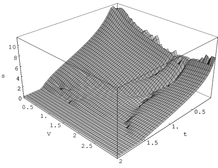
FIG. 2.: The largest inverse order-localization length $s_{1}$ for the first numerical LQI $A_{1}$ ($p=13$) vs. parameters $t,V$.

$p$	2	3	4	5	6	7	8	9	10	11	12	13	14
$d_{p}$	3	5	7	11	16	26	41	67	108	179	294	495	832
$d_{p,0}$	1	2	3	5	6	10	13	23	34	61	92	163	258
$d_{p,1}$	1	2	1	5	2	10	7	21	22	51	66	137	202

TABLE I.: Dimensions of truncated MILA ${\mathfrak{S}}_{p}$, and of nullspaces of ${\rm\bf H}_{p,\alpha}$, for different orders of truncation $p$.

Further, we use a theorem of Mazur [5] generalized by Suzuki [6] (MS) to compute canonical averages [9] of time averaged correlation functions of certain observables. We consider dimensionless kinetic energy $T=H_{1}$, where $\langle T\rangle=(1|T)=1$, with time-correlator

$$D=\lim_{N\rightarrow\infty}\frac{1}{N}\sum_{n=0}^{N}([T(\textstyle{\frac{1}{2}})-\langle T\rangle]|[T(n+\textstyle{\frac{1}{2}})-\langle T\rangle]).$$

MS equation expresses $D$ in terms of a sum over all LQI

$$D=\sum_{m}|(A_{m}|T)|^{2}/(A_{m}|A_{m}).$$ (7)

In case of complete integrability there are infinitely many LQI, in case of quantum ergodicity there are none and MS correlator $D$ is zero, while in intermediate regime the sum (7) (for KtV) has one or two nonzero terms. In Fig.3 we show a phase diagram of the kinetic time-correlator $D$ as determined from LQI (7). Note a sharp (phase) transition between ergodic dynamics (disordered phase $D=0$) and intermediate dynamics (ordered phase $D>0$) which may also be characterized by the maximal inverse order-localization length $s_{1}$ (Fig.2) which linearly decreases to zero at the transition. We have compared the above results on infinite KtV chains to direct calculations on finite chains of $L$ sites with periodic boundary conditions, $c_{L+1}=c_{1}$, which have a discrete quasi-energy spectrum $\eta_{n}$ and eigenstates $|n\rangle$, $U|n\rangle=\exp(-i\eta_{n})|n\rangle$. For a finite system of size $L$, a time-correlator reads

$$D_{L}=2^{-L}\sum_{n=1}^{2^{L}}({\textstyle{\frac{1}{L}}}\langle n|T|n\rangle-\langle T\rangle)^{2}.$$ (8)

However, $D_{L}$ need not necessarily converge to the proper time-correlator of an infinite system $L=\infty$, since then the time-limit $\tau\rightarrow\infty$ is taken prior to the size-limit $L\rightarrow\infty$ [1]. Nevertheless the behavior of $D_{L}$ for $L=16$ shown in Fig.4 as a function of parameters $t,V$ is very similar to the infinite system MS correlator (7) shown in Fig.3. Agreement is even quantitative, except in the region of transition between dynamical phases (Fig.5).

term	$A_{1}(t=0.2)$	$A_{2}(t=0.2)$	$A_{1}(t=1)$
$G_{1,0}$	-.9652693	-.18626	-.61162
$G_{1,1}$	-.2609845	0.65767	-.78843
$G_{3,001}$	0.0116246	-.69908	0.04195
$G_{3,101}$	0.0026499	-.02756	0.04928
$G_{5,01001}$	$2.487\cdot 10^{-4}$	0.20008	0.00507
$G_{5,01101}$	$4.200\cdot 10^{-5}$	0.00337	0.00450
$G_{5,11001}$	$4.533\cdot 10^{-5}$	0.00865	0.00487
$G_{5,11101}$	$9.884\cdot 10^{-6}$	0.00056	0.00555

TABLE II.: Coefficients of expansion of the two LQI (col.2,3) for $t=0.2,V=1$ and of the single LQI (col.4) for $t=V=1$ in terms of basis $G_{q,c}$ (col.1, $c$ is a binary code) up to 6th order. Truncation order is $p=13$. Note that all the digits shown (except possibly the last one) are the same for truncation at $p=11$. Other obsevables $G_{q,c},q=1,3,5$, are zero by construction (5).

Note that KtV map ${\hat{U}}_{\rm ad\,}$ is invariant under the parity operation ${\hat{P}}:c_{j}\rightarrow c_{-j}$ and MILA may exhaust [10] only the positive parity class, ${\hat{P}}A=A$. Unfortunately, the current $J=i(\sum_{j}c_{j}^{\dagger}c_{j+1}-h.c.)$, which, interestingly, gives rise to ideal transport in intermediate [4] (integrable [2, 3]) regime, has a negative parity ${\hat{P}}J=-J$, and hence zero overlap with the above LQI of MILA, $(A_{m}|J)=({\hat{P}}A_{m}|{\hat{P}}J)=-(A_{m}|J)=0$. However, analogous results have been found for the negative parity class of observables as well [11].

The total occupation number $N=\sum_{j}n_{j}=\textstyle{\frac{1}{2}}\sum_{j}(\sigma^{z}_{j}+1)$, is a trivial invariant of motion since $(N|{\mathfrak{S}})=(N|J)=0$. One may either consider observables over the Fock subspace of states with a fixed density $\rho:=\langle N\rangle\in[0,1]$, or as we do here using a full trace average (2), consider the entire Fock space, which is in TL equivalent to half filling, $\rho=\textstyle{\frac{1}{2}}$.

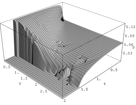
FIG. 3.: MS correlator (7) $D$ ($p=13$) vs. parameters $t,V$.

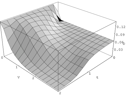
FIG. 4.: The finite size kinetic correlator (8) $D_{L}$ for $L=16$ vs. parameters $t,V$.

Conclusions: We have found strong evidence for the existence of non-trivial LQI, in a simple but generic quantum many-body system in TL, namely kicked t-V model [4]. The algebraic method, which should be applicable to other non-integrable quantum many-body systems, is based on the (computerized) construction of minimal invariant infinitely dimensional Lie algebra, MILA, generated by the essential parts of Hamiltonian (in our case, by kinetic energy and kick potential). LQI are found numerically as fixed points of the adjoint map of the evolution operator (or of the Hamiltonian if system was autonomous) in MILA. Existence of LQI is found to be fully consistent with deviations from quantum ergodicity characterized by non-vanishing averaged time-autocorrelations $D$ of a typical observable; here we use the kinetic energy. $D$ is a suitable order parameter describing the phase transition from the pseudo-integrable (intermediate) regime ($D>0$) to the quantum ergodic regime ($D=0$).

Discussions with Prof. P. Prelovšek, and the financial support by the Ministry of Science and Technology of R Slovenia are gratefully acknowledged.

FIG. 5.: The comparison between MS correlator (7) $D$ of infinite KtV chain (thick full curve) and finite size correlator (8) $D_{L}$ for $L=16$ (dotted curve) and linearly extrapolated to $1/L=0$ from data for $L=16$ and $L=12$ (dashed curve) vs. parameter $t$, and for fixed parameter $V=1$. Medium full curve and thin full curve denote separate contributions of the first and second LQI to MS correlator $D$ (7), respectively.

REFERENCES

- [1] G.Jona-Lasinio,C.Presilla,Phys.Rev.Lett.77,4322(1996).
- [2] X.Zotos, F.Naef, and P.Prelovšek, Phys.Rev.B 55, 11029 (1997).
- [3] X.Zotos and P.Prelovšek, Phys.Rev.B 53, 983 (1996); H.Castella, X.Zotos, and P.Prelovšek, Phys.Rev.Lett. 74, 972 (1995).
- [4] T.Prosen, Phys.Rev.Lett. 80, 1808 (1998).
- [5] P.Mazur, Physica 43, 533 (1969).
- [6] M.Suzuki, Physica 51, 277 (1971).
- [7] Note that non-local obervables are not normalizable in the metric (2).
- [8] Of course, at present we cannot completely exclude the possibility that such expansions are generically divergent asymptotic series.
- [9] Our example corresponds to infinite temperature, since we use a simple trace measure (2).
- [10] We have tried as well to search for LQI in the entire (huge) algebra of homogeneus observables (truncated at order ), i.e. we have numerically solved eq. (3) for the matrix of the map in the basis of observables , and we found roughly identical (and no more) numerical LQI as in MILA, although .
- [11] T.Prosen, in preparation.