Single Particle and Fermi Liquid Properties of ³He –⁴He Mixtures:
A Microscopic Analysis

Abstract

We calculate microscopically the properties of the dilute ³He component in a ³He –⁴He-mixture. These depend on both, the dominant interaction between the impurity atom and the background, and the Fermi liquid contribution due to the interaction between the constituents of the ³He component. We first calculate the dynamic structure function of a ³He impurity atom moving in ⁴He. From that we obtain the excitation spectrum and the momentum dependent effective mass. The pole strength of this excitation mode is strongly reduced from the free particle value in agreement with experiments; part of the strength is distributed over high frequency excitations. Above $k\geq 1.7$Å^-1 the motion of the impurity is damped due to the decay into a roton and a low energy impurity mode. Next we determine the Fermi–Liquid interaction between ³He atoms and calculate the pressure– and concentration dependence of the effective mass, magnetic susceptibility, and the ³He –³He scattering phase shifts. The calculations are based on a dynamic theory that uses, as input, effective interactions provided by the Fermi hypernetted–chain theory. The relationship between both theories is discussed. Our theoretical effective masses agree well with recent measurements by Yorozu et al. (Phys. Rev. B 48, 9660 (1993)) as well as those by R. Simons and R. M. Mueller (Czekoslowak Journal of Physics Suppl. 46, 201 (1996)), but our analysis suggests a new extrapolation to the zero-concentration limit. With that effective mass we also find a good agreement with the measured Landau parameter $F_{0}^{a}$.

I INTRODUCTION

Many ground state properties of ³He –⁴He mixtures, in particular the energetics of the system and the local structure, are today quite well understood both experimentally[1] and theoretically from a microscopic point of view.[2] With “microscopic” we mean that one postulates no more knowledge than the empirical Hamiltonian

$$H=-\sum_{\alpha}\sum_{i=1}^{N_{\alpha}}{\hbar^{2}\over 2m_{\alpha}}\nabla_{i}^{2}+{1\over 2}\sum_{\alpha\beta}\mathop{{\sum}^{\prime}}_{i,j}^{N_{\alpha},N_{\beta}}V(|{\bf r}_{i}^{(\alpha)}-{\bf r}_{j}^{(\beta)}|)$$ (1)

that contains only a local two-body interaction (recent work uses most frequently the Aziz[3] interaction) and the masses of the two species of particles. This paper builds on our previous studies of ground state properties of ³He –⁴He mixtures[2] and properties of single ³He impurities[4] in ⁴He. These calculations have produced an overall accuracy of the energetics of the order of a few tenths of a percent for all experimentally accessible densities and concentrations.

To specify our notation we use in the following Greek subscripts $\alpha,\beta,\ldots\in\{3,4\}$ to refer to the particle species (a ${}^{3}{\rm He}$ or a ${}^{4}{\rm He}$ particle), and Latin subscripts $i,j,\ldots$ as in the ${\bf r}_{i}$ to refer to the individual particles. The prime on the summation symbol in Eq. (1) indicates that no two pairs $(i,\alpha)$, $(j,\beta)$ can be the same. The number of particles of each species is $N_{\alpha}$, and $N=N_{3}+N_{4}$ is the total number of particles in the system. In terms of the ³He concentration $x$ we have

$$N_{3}=xN,\qquad N_{4}=(1-x)N$$ (2)

and the corresponding densities $\rho^{(\alpha)}=N_{\alpha}/\Omega$ are inversely proportional to the volume $\Omega$ occupied by the whole fluid.

The overall most successful microscopic theory of the helium liquids is the Jastrow-Feenberg variational method [5, 6] which uses a variational ansatz for the ground state wave function of the form

$$\Psi_{0}(\{{\bf r}_{i}^{(\alpha)}\}) =e^{{1\over 2}U(\{{\bf r}_{i}^{(\alpha)}\})}\Phi_{0}(\{{\bf r}_{i}^{(3)}\})$$ (3)

$$U(\{{\bf r}_{i}^{(\alpha)}\}) ={1\over 2!}\sum_{\alpha\beta}\mathop{{\sum}^{\prime}}_{i,j}^{N_{\alpha},N_{\beta}}u^{(\alpha\beta)}({\bf r}_{i},{\bf r}_{j})+{1\over 3!}\sum_{\alpha\beta\gamma}\mathop{{\sum}^{\prime}}_{i,j,k}^{N_{\alpha},N_{\beta},N_{\gamma}}u^{(\alpha\beta\gamma)}({\bf r}_{i},{\bf r}_{j},{\bf r}_{k})\ .$$ (4)

Here $\Phi_{0}(\{{\bf r}_{i}^{(3)}\})$ is the Slater determinant of plane waves ensuring the antisymmetry of the Fermion component of the wave function. The functions $u^{(\alpha\beta)}({\bf r}_{i},{\bf r}_{j})$ and $u^{(\alpha\beta\gamma)}({\bf r}_{i},{\bf r}_{j},{\bf r}_{k})$ are the pair and triplet correlations; the species superscripts determine the type of correlation. An essential part of the method is the optimization of the ground state correlations by the variational principles [7, 8, 9]

$${\delta E_{0}\over\delta u^{(\alpha\beta)}({\bf r}_{i},{\bf r}_{j})}=0\,,\qquad{\delta E_{0}\over\delta u^{(\alpha\beta\gamma)}({\bf r}_{i},{\bf r}_{j},{\bf r}_{k})}=0\;,$$ (5)

where

$$E_{0}={\langle\Psi_{0}|H|\Psi_{0}\rangle\over\langle\Psi_{0}|\Psi_{0}\rangle}$$ (6)

is the variational energy expectation value. Details of the procedure, and the necessary working formulas have been discussed at length in Ref. [2].

II DYNAMICS OF A SINGLE ³HE ATOM

This section briefly reviews our method [10, 4] to calculate the dynamics of an impurity atom in the host liquid ⁴He in its ground state with the wave function $\Psi({\bf r}_{1},...,{\bf r}_{N})$. The Jastrow-Feenberg wave function for the ground state of a single impurity atom in ⁴He is easily derived from the wave function (4) by setting $N_{3}=1$ and the Slater determinant $\Phi_{0}({\bf r}_{0})$ equal to unity,

$$\Psi^{(3)}({\bf r}_{0},{\bf r}_{1},...,{\bf r}_{N})=\exp{1\over 2}\Bigl{[}\sum_{j=1}^{N}u^{(34)}({\bf r}_{0},{\bf r}_{j})+{1\over 2!}\mathop{\sum_{j,k=1}}_{j\neq k}^{N}u^{(344)}({\bf r}_{0},{\bf r}_{j},{\bf r}_{k})\Bigr{]}\Psi({\bf r}_{1},...,{\bf r}_{N})\ .$$ (7)

The coordinate ${\bf r}_{0}$ refers to the ³He atom and ${\bf r}_{1}\ldots{\bf r}_{N}$ to the ⁴He atoms. Results for ground state calculations with this wave function have been reported elsewhere.[4] They are consistent with the low concentration limit of the calculations of Ref. [2] and in quantitative agreement with experiments.

The dynamics of an impurity atom is determined by its response to a weak, external time–dependent perturbation $U_{\rm ext}({\bf r}_{0};t)$. A natural generalization of the wave function (7) for a moving impurity atom is to allow for time-dependent correlations. The kinematic and dynamic correlations are separated by writing the wave function in the form

$$\Phi(t)=e^{-iE_{N+1}t/\hbar}\;\Psi^{(3)}({\bf r}_{0},{\bf r}_{1},...{\bf r}_{N};t)/\sqrt{\left\langle\Psi^{(3)}(t)\mid\Psi^{(3)}(t)\right\rangle}\ ,$$ (8)

where $E_{N+1}$ is the variational ground state energy of the $N+1$ particle system, and $\Psi^{(3)}({\bf r}_{0},{\bf r}_{1},...{\bf r}_{N};t)$ contains the time–dependent correlations,

$$\Psi^{(3)}({\bf r}_{0},{\bf r}_{1},...{\bf r}_{N};t)=\exp{1\over 2}\Bigl{[}\delta u^{(3)}({\bf r}_{0};t)+\sum_{i=1}^{N}\delta u^{(34)}({\bf r}_{0},{\bf r}_{i};t)\Bigr{]}\Psi^{(3)}({\bf r}_{0},{\bf r}_{1},...,{\bf r}_{N})\ .$$ (9)

The time–dependent components of the wave function are determined by an action principle, searching for a stationary value of the action integral

$${\cal L}=\int\!dt\;\langle\Phi(t)|H^{(3)}+U_{\rm ext}({\bf r}_{0};t)-i\hbar{\partial\over\partial t}|\Phi(t)\rangle\ ,$$ (10)

where $H^{(3)}$ is the Hamiltonian of the impurity-background system, obtained from Eq. (1) for $N_{3}=1$.

We make two assumptions in the evaluation of the action integral. First we require that the pair– and triplet correlation functions in the ground state are optimized. This is important because it eliminates all contributions to the action integral (10) that are linear in the time-dependent correlation functions. Then we assume that the perturbation is weak which allows us to keep only the quadratic terms in $\delta u^{(3)}({\bf r}_{0};t)$ and $\delta u^{(34)}({\bf r}_{0},{\bf r}_{i};t)$. The expression (10) simplifies because the potential energy term commutes with the time–dependent part of the wave function and we are left with second-order terms originating from the kinetic energy and the time derivative only.[10, 4]

The variation of the action integral with respect to $\delta u^{(3)}({\bf r}_{0};t)$ and $\delta u^{(34)}({\bf r}_{0},{\bf r}_{i};t)$ leads to one- and two-particle continuity equations, respectively, [10, 4]

$$\nabla_{0}\cdot{\bf j}^{(3)}({\bf r}_{0};t)+{\partial\over\partial t}\delta\rho^{(3)}({\bf r}_{0};t)={2\rho^{(3)}\over\hbar}U_{\rm ext}({\bf r}_{0};t)$$ (11)

$$\nabla_{0}\cdot{\bf j}^{(34)}({\bf r}_{0},{\bf r}_{1};t)+\nabla_{1}\cdot{\bf J}^{(34)}({\bf r}_{0},{\bf r}_{1};t)+{\partial\over\partial t}\delta\rho^{(34)}({\bf r}_{0},{\bf r}_{1};t)={2\over\hbar}U_{\rm ext}({\bf r}_{0};t)\rho^{(34)}({\bf r}_{0},{\bf r}_{1})\ .$$ (12)

We have kept only the time dependent parts of the full densities. The transition currents are defined in terms of the fluctuating one-particle density and pair correlation function:

$${\bf j}^{(3)}({\bf r}_{0};t) ={\hbar\over 2m_{3}i}\biggl{[}\nabla_{0}\delta\rho^{(3)}({\bf r}_{0};t)-\int\!d^{3}r_{1}\;\delta u^{(34)}({\bf r}_{0},{\bf r}_{1};t)\nabla_{0}\rho^{(34)}({\bf r}_{0},{\bf r}_{1})\biggr{]},$$ (13)

$${\bf j}^{(34)}({\bf r}_{0},{\bf r}_{1};t) ={1\over\rho^{(3)}}{\bf j}^{(3)}({\bf r}_{0};t)\rho^{(34)}({\bf r}_{0},{\bf r}_{1})+{\hbar\over 2m_{3}i}\Biggl{[}\rho^{(34)}({\bf r}_{0},{\bf r}_{1})\nabla_{0}\delta u^{(34)}({\bf r}_{0},{\bf r}_{1};t)$$ (14)

$$+\int\!d^{3}r_{2} \Bigl{[}\rho^{(344)}({\bf r}_{0},{\bf r}_{1},{\bf r}_{2})-{1\over\rho^{(3)}}\rho^{(34)}({\bf r}_{0},{\bf r}_{1})\rho^{(34)}({\bf r}_{0},{\bf r}_{2})\Bigr{]}\nabla_{2}\delta u^{(34)}({\bf r}_{0},{\bf r}_{2};t)\Biggr{]}\ ,$$ (15)

$${\bf J}^{(34)}({\bf r}_{0},{\bf r}_{1};t) ={\hbar\over 2m_{4}i}\rho^{(34)}({\bf r}_{0},{\bf r}_{1})\nabla_{1}\delta u^{(34)}({\bf r}_{0},{\bf r}_{1};t)\ .$$ (16)

¿From the calculation of the ground state properties of the impurity we need here the impurity-background pair and triplet distribution functions $\rho^{(34)}({\bf r}_{0},{\bf r}_{1})$ and $\rho^{(344)}({\bf r}_{0},{\bf r}_{1},{\bf r}_{2})$, respectively.

We assume that an infinitesimal external potential drives the system with a given frequency and wavelength, and the system responds with a density fluctuations of the same frequency and wavelength. This determines the linear response function

$$\chi^{(3)}(k,\omega)={\delta\rho^{(3)}(k,\omega)\over\rho^{(3)}\tilde{U}_{\rm ext}(k,\omega)}\ .$$ (17)

The inverse of the response function can be calculated from the Fourier transform of the continuity equations. The Fourier transform of the density fluctuations is defined as follows

$$\delta\rho^{(3)}(k,\omega) = \int\!d^{3}r_{0}\,dt\;e^{-i({\bf k}\cdot{\bf r}_{0}-\omega t)}\delta\rho^{(3)}({\bf r}_{0};t)\ ,$$ (18)

and analogously for the external potential.

The poles of $\chi^{(3)}(k,\omega)$ determine the elementary excitations; their dispersion relation is obtained from the first continuity equation by setting $\tilde{U}_{\rm ext}(k,\omega)=0$. This leads to the implicit equation

$$\hbar\omega={\hbar^{2}k^{2}\over 2m_{3}}+\Sigma^{(3)}(k,\omega)$$ (19)

with the self-energy

$$\Sigma^{(3)}(k,\omega)={\hbar^{2}\over 2m_{3}}\int{d^{3}p\over(2\pi)^{3}\rho^{(4)}}\;{{\bf k}\cdot{\bf p}\;S^{(34)}(p)\beta^{(34)}_{{\bf k},\omega}({\bf p})\over\Bigl{[}\hbar\omega-t^{(3)}({\bf k}+{\bf p})-\epsilon^{(4)}(p)\Bigr{]}}\ .$$ (20)

Here $S^{(34)}(p)$ is the ³He –⁴He structure function, $t^{(3)}(k)$ the kinetic energy of the impurity and $\epsilon^{(4)}(p)$ the background phonon-roton spectrum. The function $\beta^{(34)}_{{\bf k},\omega}({\bf p})$ will be defined below.

The linear response function has then a simple form

$$\chi^{(3)}(k,\omega)={1\over\hbar\omega-t^{(3)}(k)-\Sigma^{(3)}(k,\omega)+i\eta}-{1\over\hbar\omega+t^{(3)}(k)+\Sigma^{(3)}(k,\omega)+i\eta},~{}~{}\eta\rightarrow 0+\;.$$ (21)

This is the density–density response function of the ³He component in the dilute limit. The response function is related to the Green’s function through[11]

$$\chi^{(3)}(k,\omega)=-i\int{d^{3}q\;d(\hbar\omega^{\prime})\over(2\pi)^{4}}\;G(q,\omega^{\prime})\;G({\bf k}+{\bf q},\omega^{\prime}+\omega)\;,$$ (22)

where

$$G(q,\omega)={1-n_{\bf q}\over\hbar\omega-t^{(3)}(q)-\Sigma^{(3)}(q,\omega)+i\eta}+{n_{\bf q}\over\hbar\omega-t^{(3)}(q)-\Sigma^{(3)}(q,\omega)-i\eta},~{}~{}\eta\rightarrow 0+$$ (23)

and $n_{\bf q}$ is the Fermi distribution. In the dilute limit, we have $n_{\bf q}=\delta_{{\bf q},0}$ and Eq. (22) reduces to Eq. (21) or, vice versa, the first part of Eq. (21) can also be regarded as the single–particle Green’s function.

The imaginary part of the linear response function defines the dynamic structure function

$$S(k,\omega)=-{1\over\pi}\Im m\,[\chi^{(3)}(k,\omega)]\;,$$ (24)

which can be measured in scattering experiments.

The contributions of the elementary excitations can be separated out as a delta-function,

$$S(k,\omega)=Z(k)\delta(\hbar\omega-\hbar\omega_{p})+S_{\rm m}(k,\omega)\ .$$ (25)

Here $\hbar\omega_{p}$ is the solution of Eq. (19) and $S_{\rm m}(k,\omega)$ is the contribution of the modes that make the self energy complex. This becomes possible when the denominator in Eq. (20) becomes positive for some value of ${\bf p}$,

$$\max_{\bf p}\left[\hbar\omega-t^{(3)}({\bf k}+{\bf p})-\epsilon^{(4)}(p)\right]~{}>~{}0\ .$$ (26)

If the condition (26) is satisfied, then it is kinematically possible that the ³He impurity loses energy by emitting a phonon-roton mode $\epsilon^{(4)}(p)$ while making a transition into a low-energy impurity mode $t^{(3)}({\bf k}+{\bf p})$. The strength of the pole $Z(k)$ can be evaluated from the derivative of the self energy,

$$Z(k)=\left[1-\left.{d\Sigma^{(3)}(k,\omega)\over d(\hbar\omega)}\right|_{\omega=\omega_{p}}\right]^{-1}\ .$$ (27)

The second continuity equation (12) can be written in the Fourier space and formulated as a linear integral equation for $\beta^{(34)}_{{\bf k},\omega}({\bf p})$, which is related to the fluctuating pair correlation function as discussed in the Appendix. The integral equation sums ladder diagrams up to infinite order,

$$\beta^{(34)}_{{\bf k},\omega}({\bf p})=\hbar\omega\;\frac{{\bf k}\cdot{\bf p}}{k^{2}}\;\frac{S^{(34)}(p)}{S^{(44)}(p)}-\int{d^{3}q\over(2\pi)^{3}\rho^{(4)}}\;\frac{\beta^{(34)}_{{\bf k},\omega}({\bf q})K_{{\bf k},\omega}({\bf p},{\bf q})}{\Bigl{[}\hbar\omega-t^{(3)}({\bf k}+{\bf q})-\epsilon^{(4)}(q)\Bigr{]}}$$ (28)

with the kernel

$$K_{{\bf k},\omega}({\bf p},{\bf q}) = S^{(44)}(q)\Biggl{\{}\left[\left(S^{(34)}(|{\bf p}-{\bf q}|)+1\right)\tilde{u}^{(344)}({\bf p}-{\bf q},-{\bf p},{\bf q})+S^{(34)}(|{\bf p}-{\bf q}|)\right]$$ (29)

$$\times \left[\hbar\omega-\frac{({\bf k}+{\bf p})\cdot({\bf k}+{\bf q})}{p^{2}}t^{(3)}(p)\right]\Biggr{\}}-S^{(34)}(|{\bf p}-{\bf q}|)\frac{{\bf p}\cdot{\bf q}}{p^{2}}\epsilon^{(4)}(p)\ .$$ (30)

Here we need the static structure function $S^{(44)}(k)$ of the background and the triplet correlation function $\tilde{u}^{(344)}$ with one impurity. Details of the derivation of the above equation are given in the Appendix.

The singularity structure of Eq. (28) is the same as that of the self energy. For real frequencies $\omega$ the imaginary part of $\beta^{(34)}_{{\bf k},\omega}({\bf q})$ is zero if the energy denominator is negative for all values of ${\bf q}$. Modes with an energy $\hbar\omega$ high enough to satisfy the inequality (26) can decay into a phonon-roton mode and the solution has a non-zero imaginary part.

The long-wavelength limit of the excitation energy defines the hydrodynamic effective mass $m^{*}_{H}$.

$$\hbar\omega={\hbar^{2}k^{2}\over 2m^{*}_{H}}\ ,~{}~{}{\rm when}~{}~{}k\to 0\ .$$ (31)

Inserting this into Eq. (19) we get

$${m^{*}_{H}\over m_{3}}={1\over 1-I}$$ (32)

with

$$I=\lim_{k\rightarrow 0+}{1\over k^{2}}\int{d^{3}p\over(2\pi)^{3}\rho^{(4)}}\;{{\bf k}\cdot{\bf p}\;S^{(34)}(p)\;\beta^{(34)}_{{\bf k},\omega_{0}}({\bf p})\over t^{(3)}(p)+\epsilon^{(4)}(p)}\ ,$$ (33)

where $\omega_{0}=\hbar k^{2}/2m^{*}_{H}$. Using Eq. (31) we find that in the long-wavelength limit the pole strength is inversely proportional to the effective mass,

$$\lim_{k\rightarrow 0}Z(k)={m_{3}\over m^{*}_{H}}\ .$$ (34)

In the so-called “uniform limit approximation”[5] one neglects all coordinate-space products of two functions, i.e. we approximate, for example, $\rho^{(34)}({\bf r}_{0},{\bf r}_{1})\delta u^{(34)}({\bf r}_{0},{\bf r}_{1})\approx\rho^{(3)}\rho^{(4)}\delta u^{(34)}({\bf r}_{0},{\bf r}_{1})$, but convolution products are retained. Then, $\beta^{(34)}_{{\bf k},\omega_{0}}({\bf p})$ has a simple form[4]

$$\beta^{(34)}_{{\bf k},\omega_{0}}({\bf p})={\hbar^{2}\over 2m_{3}}\;{\bf k}\cdot{\bf p}\;{S^{(34)}(p)\over S^{(44)}(p)}\ .$$ (35)

This together with the equations (32) and (33) gives the “un-renormalized effective mass” derived by Owen.[12]

III FERMI LIQUID INTERACTIONS

Up to this point, we have considered only the interaction of one single ³He atom with the host liquid. Further interesting effects arise from the interaction between pairs of ³He atoms and the specific dynamics imposed on the ³He component by the Pauli principle.[13] The most obvious manifestations of interactions between the ³He atoms are magnetic properties[14] and corrections to the hydrodynamic mass. Both effects provide interesting problems from the point of view of low-temperature experiments as well as microscopic many–body theory.

The dilute mixture is a particularly attractive system for the theorist because many of the complicated exchange effects that obscure the theory of pure ³He are negligible. A new effect is that the interaction between ³He atoms is dominated by the exchange of phonons through the host liquid[14, 15, 16] and therefore depends not only on the relative momentum between the two particles, but also on the momentum of each individual particle relative to the ⁴He background.

Small perturbations of the ground state of a normal, interacting Fermi liquid are described within Landau’s Fermi Liquid theory.[13] The energy $E_{0}$ of the system is considered to be a functional of the quasiparticle occupation numbers $n_{{\bf k},\sigma}$, and the quasiparticle energies are, close to the ground state, given by the variations of that energy with respect to $n_{{\bf k},\sigma}$. Thus, the quasiparticle spectrum is

$$\epsilon^{(3)}({\bf k},\sigma)={\delta E_{0}\over\delta n_{{\bf k},\sigma}}\ .$$ (36)

For a symmetric ground state, the $\epsilon^{(3)}({\bf k},\sigma)$ are spin–independent; we shall suppress the spin argument whenever possible.

In the mixture, the single particle spectrum consists of two parts. The first is the hydrodynamic interaction of a single impurity atom with the background, leading to the “hydrodynamic effective mass” $m^{*}_{H}$ as discussed in the preceding section. The second part is due to the interaction with other ³He atoms. Hence, we can split the quasiparticle spectrum (36) into two pieces,

$$\epsilon^{(3)}(k)=\epsilon^{(3)}_{H}(k)+\epsilon^{(3)}_{\rm QP}(k)\ ,$$ (37)

Correspondingly, the total effective mass of the ³He particles is

$${\hbar^{2}k_{F}\over m^{*}}\equiv{\hbar^{2}k_{F}\over m^{*}_{H}}+\left.{d\over dk}\epsilon^{(3)}_{\rm QP}(k)\right|_{k=k_{F}}\ ,$$ (38)

where $k_{F}$ is the Fermi momentum of the ³He component.

Interactions between the ³He atoms are, to the extent that the ³He atoms remain close to the Fermi surface, described by Landau’s Fermi liquid (“quasiparticle”) interaction which is the second variation

$$f_{{\bf k}\sigma,{\bf k}^{\prime}\sigma^{\prime}}^{\rm var}={\delta\epsilon^{(3)}({\bf k},\sigma)\over\delta n_{{\bf k}^{\prime},\sigma^{\prime}}}=\left.{\delta^{2}E_{0}\over\delta n_{{\bf k},\sigma}\delta n_{{\bf k}^{\prime},\sigma^{\prime}}}\right|_{n_{k}^{(0)}}\ ,$$ (39)

evaluated at the ground state momentum distribution $n_{k}^{(0)}=\theta(k_{F}-k)$. The quasiparticle interaction normally contains a spin-independent and a spin-dependent part,

$$f_{{\bf k}\sigma,{\bf k}^{\prime}\sigma^{\prime}}^{\rm var} = f_{{\bf k},{\bf k}^{\prime}}^{\rm s}+f_{{\bf k},{\bf k}^{\prime}}^{\rm a}\;\mathbf{\sigma}\cdot\mathbf{\sigma}^{\prime}\,,$$ (40)

which is also frequently written as

$$f_{{\bf k},{\bf k}^{\prime}}^{\rm s(a)}={1\over 2}\left(f_{\uparrow,\uparrow}^{\rm var}\pm f_{\uparrow,\downarrow}^{\rm var}\right)\,;$$ (41)

the $\mathbf{\sigma}$’s are Pauli spin matrices. Since the quasiparticle interaction is to be taken for $\left|{\bf k}\right|=\left|{\bf k}^{\prime}\right|=k_{F}$, it depends only on the angle between ${\bf k}$ and ${\bf k}^{\prime}$, and it is convenient to expand that dependence in Legendre polynomials

$$f_{{\bf k},{\bf k}^{\prime}}^{\rm s(a)}=\sum_{\ell}f_{\ell}^{s(a)}P_{\ell}(\hat{\bf k}\cdot\hat{\bf k}^{\prime})\,.$$ (42)

The strength of the interaction relative to the kinetic energy is measured by the dimensionless quantities

$$F_{\ell}^{\rm s(a)}=N(0)\;f_{\ell}^{\rm s(a)}={\Omega\;m^{*}\;k_{F}\over\pi^{2}\;\hbar^{2}}\;f_{\ell}^{\rm s(a)}\;,$$ (43)

where $N(0)$ is the density of states at the Fermi surface.

At this point, the quasiparticle contribution to the effective mass is normally related to the Landau parameter $f_{1}^{s}$ or $F_{1}^{s}$. To derive this relationship, one must assume Galilean–invariance of the whole liquid. As already observed by Baym and Pethick,[17] the argument must be treated with caution here because, while the whole mixture is Galilean invariant, the properties of the ³He component are not invariant against motion relative the ⁴He background. This becomes relevant when one attempts to treat the phonon–mediated processes as an effective interaction between the ³He atoms: As long as this interaction is assumed to be static, it can depend only on the properties of the participating ³He particles. However, in reality the interaction is dominated by the dynamic exchange of phonons through the background liquid and the motion of the interacting particles relative to that background becomes important. The correct definition of the effective mass is therefore the one of Eq. (38); we will explicitly see the effect of the retardation of the quasiparticle interaction in our numerical applications.

The magnetic response is determined by the change of the quasiparticle energy when a magnetic field $H$ is applied. Since the ⁴He background does not couple to the spin degrees of freedom, the $\delta\epsilon^{(3)}({\bf k},\sigma)$ depends, to first order in the magnetic field, only on the spin—populations $n_{{\bf k},\sigma}$. Hence the usual relationship of Landau theory,

$${\chi^{*}_{\sigma,\rm ideal}\over\chi_{\sigma}} = {m_{H}^{*}\over m^{*}}\;\left(1+{m^{*}\;k_{F}\over\pi^{2}\;\hbar^{2}}\,\Omega\,f_{0}^{\rm a}\right)={m_{H}^{*}\over m^{*}}\;\left(1+F_{0}^{\rm a}\right)\;,$$ (44)

between the $F_{0}^{\rm a}$ and the spin–susceptibility is applicable. In order to separate the hydrodynamic “backflow” effect from the Fermi liquid interaction, we have defined here $\chi^{*}_{\sigma,\rm ideal}$ as the Pauli susceptibility for ³He particles with mass $m_{H}^{*}$.

A Variational Fermi Liquid Theory

Landau’s Fermi liquid theory is phenomenological in the sense that it relates Fermi liquid parameters to physical observables, and derives relationships between different physical observables, but it makes no statements on how to compute these quantities. Methods to calculate the quasiparticle excitations and interactions from the underlying Hamiltonian (1) of the system are provided by microscopic many-body theory.

At the level of the variational theory, the single particle excitation spectrum is calculated by allowing for an occupation of single particle orbitals $n_{{\bf k},\sigma}$ in the Slater function $\Phi_{0}$ that is different from the Fermion ground state $n_{k}^{(0)}$. The graphical analysis of the functional derivatives has been carried out in Ref. [18]; the variational single-particle field $u(k)$ has the general form

$$\epsilon^{(3)}(k,\sigma)=t^{(3)}(k)+u(k)+U_{0}\,,$$ (45)

where $U_{0}$ is a constant determined by the chemical potential, and $u(k)$ a momentum dependent average field. In the present dilute case, the average field can be written in the form of a Hartree-Fock field

$$u(k)=-~{}{\rho^{(3)}\over 2}\int d^{3}r\,W_{\rm eff}(r)\,j_{0}(r\,k)\,\ell(r\,k_{F})$$ (46)

where $\ell(x)=3~{}j_{1}(x)/x$ is the Fermi exchange function familiar from Hartree-Fock theory, and $W_{\rm eff}(r)$ is a local effective interaction which can be constructed diagrammatically by the summation of (F)HNC diagrams in the mixture. [2, 18] For further reference, we also formulate the average field in momentum space,

$$u(k)=-\int{d^{3}q\over(2\pi)^{3}\rho^{(3)}}\,n_{|{\bf q}-{\bf k}|,\sigma}\,\tilde{W}_{\rm eff}(q)\,,$$ (47)

where $\tilde{W}_{\rm eff}(q)$ is the dimensionless Fourier transform $\tilde{W}_{\rm eff}(q)=\rho^{(3)}\int d^{3}rW_{\rm eff}(r)\exp(i\;{\bf k}\cdot{\bf r})$.

In the same approximation, the quasiparticle interaction can also be expressed, up to an additive constant, in terms of the effective interaction $W_{\rm eff}(r)$:

$$f_{{\bf k}\sigma,{\bf k}^{\prime}\sigma^{\prime}}^{\rm var} = {1\over\Omega}\left[{\rm const.}-\delta_{\sigma,\sigma^{\prime}}\,\tilde{W}_{\rm eff}(|{\bf k}-{\bf k^{\prime}}|)\right]$$ (48)

$$= f_{{\bf k},{\bf k}^{\prime}}^{\rm s}+f_{{\bf k},{\bf k}^{\prime}}^{\rm a}\;\mathbf{\sigma}\cdot\mathbf{\sigma}^{\prime}\,.$$ (49)

The constant first term in Eq. (49) comes from the variation of $U_{0}$ with respect to the occupation number $n_{{\bf k},\sigma}$; it is related to the compressibility of the ³He component and is therefore not our concern now.

B Correlated Basis Functions

It has been known for quite some time[19] that the naïve implementation of the FHNC/EL theory (or, for that matter, any variational wave function of the type (4)) to the problem of pure ³He has a number of severe problems. One is that it leads to an effective mass of pure ³He that is less than one[20] which is in sharp contrast to experiments.[21, 22] Another problem is that it predicts an instability against spontaneous spin-polarization. The physics of mixtures is, of course, entirely different from that of a pure ³He liquid. But we will see that the technical approximations implicit to the Jastrow-Feenberg wave function (4) lead to practically the same problems in the mixture.

The deficiencies of the variational theory are, as we shall see more explicitly below, due to the fact that the wave function (4) describes the average correlations between particles quite well, whereas it is insensitive to the specifics of the correlations in the vicinity of the Fermi surface. The cure for the problem is known to be Correlated-Basis Functions (CBF) theory.[5] A complete, non-orthogonal basis of the Hilbert space is built on the ground state wave function (4) by defining

$$\Psi_{m}(\{{\bf r}_{i}^{(\alpha)}\})=e^{{1\over 2}U(\{{\bf r}_{i}^{(\alpha)}\})}\Phi_{m}(\{{\bf r}_{i}^{(3)}\})\ ,$$ (50)

where the $\left\{\Phi_{m}(\{{\bf r}_{i}^{(3)}\})\right\}$ is a complete set of Slater determinants for the ³He component. Within the basis $\left\{\Psi_{m}(\{{\bf r}_{i}^{(\alpha)}\})\right\}$, perturbative expansions can be derived in much the same way as in conventional Rayleigh-Schrödinger perturbation theory, and diagrammatic structures like ring-, ladder-, or self–energy diagrams can be defined and summed to infinite order. Note that perturbative corrections are applied to the Fermion components only; this is legitimate since the Jastrow-Feenberg wave function is in principle exact for Bosons, whereas it is not exact for Fermions.

The general strategy of CBF theory has been described in detail in many places;[5] the basic results needed for our analysis have been derived in Ref. [23]. Without going into the details of that theory, we assert that there is a one-to-one correspondence between the compound-diagrammatic elements of the FHNC theory and that of ordinary, Green’s functions based perturbation theory. Loosely speaking, CBF theory can be interpreted as a microscopic procedure for the calculation of static effective interactions. For our purpose, the application of CBF theory can be summarized simply by stating that, in the evaluation of the energy, the chain-diagrams of FHNC theory are replaced by the ring-diagrams of the RPA theory, using a diagrammatically defined static effective interaction which we identify with the “particle-hole interaction”.

Since we are predominantly interested in variations of the energy, we can formulate the theory in terms of a Green’s functions approach where the effective interactions come from the FHNC analysis, examine the relationships between the FHNC and the CBF approximation, and compare the results of different theories.

In perturbative theories, single particle properties are described by a complex self-energy $\Sigma(k,\omega)$; the single particle spectrum $\varepsilon(k)$ is obtained from the solution of the equation

$$\varepsilon(k)=t^{(3)}(k)+\Sigma(k,\varepsilon(k)/\hbar)\ .$$ (51)

If only single phonon coupling processes are considered, the self-energy $\Sigma(k,E)$ is given in the so-called G0W-approximation[24, 25]

$$\Sigma(k,\omega)=i\int{d^{3}qd(\hbar\omega^{\prime})\over(2\pi)^{4}\rho^{(3)}}\,G^{(0)}(\left|{\bf k}-{\bf q}\right|,\omega-\omega^{\prime})\,\tilde{V}_{\rm eff\/}(q,\omega^{\prime})$$ (52)

where

$$G^{(0)}(k,\omega)={1-n_{{\bf k},\sigma}\over\hbar\omega-t^{(3)}(k)+i\eta}+{n_{{\bf k},\sigma}\over\hbar\omega-t^{(3)}(k)-i\eta}$$ (53)

is the free single-particle Green’s function and

$$\tilde{V}_{\rm eff\/}(q,\omega)=\tilde{V}_{\rm p-h}^{(33)}(q)+\sum_{\alpha\beta}\tilde{V}_{\rm p-h}^{(3\alpha)}(q)\,\chi^{(\alpha\beta)}(q,\omega)\,\tilde{V}_{\rm p-h}^{(3\beta)}(q)$$ (54)

is the effective, energy dependent ³He –³He interaction. In Eq. (54), the $\tilde{V}_{\rm p-h}^{\alpha\beta}(q)$ are the local, particle-hole irreducible interactions, and $\chi^{(\alpha\beta)}(q,\omega)$ is the density-density response matrix. In fact, the G0W approximation is simply the variation of an RPA energy expectation value with respect to a single particle Green’s function. The key quantities $\tilde{V}_{\rm p-h}^{\alpha\beta}(q)$ can in principle be defined diagrammatically in Green’s functions based theories, but it is impractical to calculate these interactions without further approximations. CBF perturbation theory solves this problem by giving unambiguous prescriptions[2] for the calculation of static approximations for these quantities.

To separate the “hydrodynamic” and the “Fermionic” component of the self-energy, we rewrite the single-particle Green’s function as

$$G^{(0)}(k,\omega) = {1\over\hbar\omega-t^{(3)}(k)+i\eta}+n_{{\bf k},\sigma}\left[-{1\over\hbar\omega-t^{(3)}(k)+i\eta}+{1\over\hbar\omega-t^{(3)}(k)-i\eta}\right]$$ (55)

$$\equiv G_{H}^{(0)}(k,\omega)+G_{F}^{(0)}(k,\omega)$$ (56)

and the self-energy in the form

$$\Sigma(k,\omega) = \Sigma_{H}(k,\omega)+\Sigma_{F}(k,\omega),$$ (57)

$$\Sigma_{H}(k,\omega) = i\int{d^{3}q\,d(\hbar\omega^{\prime})\over(2\pi)^{4}\,\rho^{(3)}}\;G_{H}^{(0)}(\left|{\bf k}-{\bf q}\right|,\omega-\omega^{\prime})\;\tilde{V}_{\rm eff\/}(q,\omega^{\prime}),$$ (58)

$$\Sigma_{F}(k,\omega) = i\int{d^{3}q\,d(\hbar\omega^{\prime})\over(2\pi)^{4}\,\rho^{(3)}}\;G_{F}^{(0)}(\left|{\bf k}-{\bf q}\right|,\omega-\omega^{\prime})\;\tilde{V}_{\rm eff\/}(q,\omega^{\prime})\ .$$ (59)

The “hydrodynamic” part (58) of the self-energy leads, in the dilute limit $\rho^{(3)}\rightarrow 0$, to an effective mass that is identical[4] to the one obtained in the previous section in the “uniform limit approximation” derived in Eqs. (32) and (35). This approximation is quantitatively not quite sufficient, but it contains, at a semi-quantitative level, the basic physics of impurity motion, in particular the coupling of the impurity to the excitations of the host liquid. The method of time–dependent correlation functions described in Sec. II introduces a systematic procedure to improve upon this approximation.

Let us now focus on the Fermion term, Eq. (59). The energy integration yields the compact form

$$\Sigma_{F}(k,\omega)=-\int{d^{3}q\over(2\pi)^{3}\rho^{(3)}}\,n_{|{\bf q}-{\bf k}|,\sigma}\,\tilde{V}_{\rm eff\/}(q,\omega-t^{(3)}({\bf k}-{\bf q})/\hbar)\,.$$ (60)

To calculate the spin-susceptibility we can directly apply Eqs. (43) and (44) and arrive at

$$\Omega f_{0}^{\rm a}=-{1\over 2\rho^{(3)}}\int\!\!\int{d\theta\;d\phi\over 4\pi}\;\sin(\theta)\;\tilde{V}_{\rm eff\/}(|{\bf k}_{\rm F}-{\bf k^{\prime}}_{\rm F}|,0)\,.$$ (61)

In principle, we would also need to calculate the variation of the kinetic energy $t^{(3)}({\bf k}-{\bf q})$ with respect to the quasiparticle occupation number $n_{{\bf k},\sigma}$, but in the dilute limit of the mixture, this quantity is dominated by the hydrodynamic backflow relative to the background and can, to good approximation, be replaced by a free single–particle spectrum with an effective mass $m_{H}^{*}$.

The comparison of Eqs. (61) and (60) demonstrates the difference between the Landau effective mass that would be calculated from the $\ell=1$ equivalent to Eq. (61), and the momentum derivative $\left.d\varepsilon(k,\sigma)/dk\right|_{k=k_{F}}$. In the latter case, one also includes the momentum dependence of the energy appearing in the effective interaction $\tilde{V}_{\rm eff\/}(q,\omega-t^{(3)}({\bf k}-{\bf q})/\hbar)$.

We have now reached the point where the quasiparticle interaction is expressed in terms of a local, but energy dependent effective interaction very similar to the FHNC theory, cf. Eq. (49). The relationship to Eq. (47) is now apparent: $\Sigma_{F}(k,\omega)$ could be rewritten as a Hartree-Fock expression of the form (47) if the effective interaction $\tilde{V}_{\rm eff\/}(q,\omega)$ were energy independent. The question that arises naturally is what the relationship between the energy-independent effective interaction $\tilde{W}_{\rm eff}(q)$ and the energy dependent interaction $\tilde{V}_{\rm eff}(q,\omega)$ is. We will address this question in the next subsection.

C Connection between HNC and CBF Theories

We here outline the general manipulations that lead from the compound-diagrammatic elements of the (F)HNC theory to the Green’s functions expressions. The construction of energy-independent, local effective interactions is one of the key steps in the Feynman-diagram based parquet-diagram theory[26, 27] that is needed to show the equivalence to the HNC/EL theory, and we shall demonstrate here that the relationship between (F)HNC and parquet theory reach actually farther than expected.

For simplicity, we restrict our derivation to the case of two interacting ³He impurities within the ⁴He host liquid. In this case, we need to retain only the 44-channel of the response function. In this limit, the effective interaction is

$$\tilde{V}_{\rm eff\/}(q,\omega) = \tilde{V}_{\rm p-h}^{(33)}(q)+\tilde{V}_{\rm p-h}^{(34)}(q)\;\chi^{(44)}(q,\omega)\;\tilde{V}_{\rm p-h}^{(34)}(q)$$ (62)

$$= \tilde{V}_{\rm p-h}^{(33)}(q)+\tilde{V}_{\rm p-h}^{(34)}(q)\;{\displaystyle 2t^{(4)}(q)\over(\hbar\omega)^{2}-(\epsilon^{(4)}(q))^{2}}\;\tilde{V}_{\rm p-h}^{(34)}(q)\ .$$ (63)

The prescription from parquet-theory to make this energy-dependent interaction local is as follows: Construct the RPA static structure function

$$S^{(33)}_{\rm RPA}(q) = \int{d(\hbar\omega)\over 2\pi}\;\Im m\left[\chi^{(33)}_{0}(q,\omega)+\chi^{(33)}_{0}(q,\omega)\tilde{V}_{\rm eff\/}(q,\omega)\chi^{(33)}_{0}(q,\omega)\right]$$ (64)

$$= 1-{1\over t^{(3)}(q)}\left[\tilde{V}_{\rm p-h}^{(33)}(q)-2\;{\left[V_{\rm p-h}^{(33)}(q)\right]^{2}S^{(44)}(q)\over\left(t^{(3)}(q)+\epsilon^{(4)}(q)\right)^{2}}\right]\ ,$$ (65)

where

$$\chi^{(33)}_{0}(q,\omega)={2\;t^{(3)}(q)\over(\hbar\omega)^{2}-(t^{(3)}(q))^{2}}$$ (66)

is the response function of the non-interacting ³He gas. Also, construct the ladder approximation for the same quantity in terms of a different and yet unspecified local effective interaction, say $\tilde{V}_{\rm L}(q)$

$$S^{(33)}_{\rm ladder}(q) = \int{d(\hbar\omega)\over 2\pi}\;\Im m\left[\chi^{(33)}_{0}(q,\omega)+\chi^{(33)}_{0}(q,\omega)\;\tilde{V}_{\rm L\/}(q)\chi^{(33)}_{0}(q,\omega)\right]$$ (67)

$$= 1-{1\over t^{(3)}(q)}\;\tilde{V}_{\rm L\/}(q)\ .$$ (68)

Now choose an average frequency $\bar{\omega}(q)$ such that these two forms of the static structure function are identical for

$$\tilde{V}_{\rm L\/}(q)=\tilde{V}_{\rm eff\/}(q,\bar{\omega})\ .$$ (69)

One obtains

$$(\hbar\bar{\omega})^{2}=-{\epsilon^{(4)}(q)\;(t^{(3)})^{2}(q)\over\epsilon^{(4)}(q)+2t^{(3)}(q)}\ .$$ (70)

This is the generalization of the expression given in Ref. [27] to a dilute ³He –⁴He mixture. Inserting $\hbar\bar{\omega}$ into the energy-dependent effective interaction leads directly to the FHNC approximation (46), in other words

$$\tilde{W}_{\rm eff}(q)=\tilde{V}_{\rm eff\/}(q,\bar{\omega})=\tilde{V}_{\rm L}(q)\ .$$ (71)

This final part is of a somewhat technical nature and requires the full (F)HNC formalism, in particular its use to calculate effective interactions for use in CBF theory[23, 2] and the connections with the optimization problem; it is therefore skipped here.

The equivalence (71) is the second essential theoretical result of this paper. The result is remarkable in the following sense: The concept of an “average energy” has been introduced in Refs. [26] and [27] for a one-component Bose liquid, and for finding a local approximation for the chain diagrams for the purpose of summing ladder diagrams. We find here – as in Ref. [2] – that the very same concept applies also in a different situation, namely in demonstrating the relationship between the quasiparticle interaction in FHNC theory and in the RPA. We stress that this result is an observation on how the static FHNC approximation and the G0W approximation of the self-energy are related. It does not mean that the FHNC approximation, which has been derived from looking at the static structure function, and which is capable of reproducing the static structure function with very good accuracy, is also adequate for the calculation of single-particle properties and Fermi liquid effects.

IV APPLICATIONS

A Hydrodynamic Effective Mass

The first task is the calculation of the hydrodynamic effective mass. This quantity describes the interaction of a single impurity atom with the ⁴He background. Due to the high density of the background, the G0W approximation recovers only about 80 percent of the effect and the more complete treatment of the time–dependent pair correlations described in Sec. II improves this result considerably.

One of the formal results of our analysis is that the equations (28), (20) and (30) treat the phonon-roton spectrum as a Feynman-type spectrum, $\epsilon^{(4)}(k)=\hbar^{2}k^{2}/[2m_{4}S(k)]$, which is known to lie by a factor of two too high in the roton region. To include the backflow correction also into the motion of the ⁴He particles one should add fluctuating triplet correlations into the wave function (9) and solve the triplet continuity equation. This leads to a rather complicated integral equation with uncertainty in the treatment of the four-particle distribution function. The hierarchy of continuity equations must be truncated at some tractable level. A reasonable shortcut is to modify the integral equation (28) and the self energy (20) by using the experimental phonon-roton spectrum in $\epsilon^{(4)}(k)$, replacing the impurity mass by its effective mass in the impurity kinetic energy term, $t^{(3)}(k)$, and then ignoring the higher order correlations. For the triplet distribution function we have used the convolution approximation together with the triplet correlation function as described in the Appendix.[2] The self-consistent solution of Eq. (32) leads to a rather good prediction of the hydrodynamic effective mass over the whole density regime that is experimentally accessible. The results are shown in Fig. 1 together with the fits to the measurements by Yorozu et al. [28] and Simons and Mueller [29]. More details of those results are shown in Table I, which will be discussed in the next section.

Next we need to determine the momentum dependence of the hydrodynamic effective mass; it is necessary to study this effect because at finite concentration the particles at the Fermi surface have a finite momentum. For that purpose, we have calculated the dispersion relation from Eq. (19) and have determined the “momentum dependence” of the hydrodynamic mass by writing the spectrum in the form

$$\hbar\omega_{H}(k)={\hbar^{2}k^{2}\over 2m^{*}_{H}(k)}\ .$$ (72)

In Fig. 2 we plot the quantity

$${1\over k^{2}}\Bigl{[}{m^{*}_{H}(k)\over m^{*}_{H}(0)}-1\Bigr{]}\ ,$$ (73)

which turns out to be constant for a wide momentum range implying quadratic momentum dependence of the effective mass. Our value of this constant is 0.114 at zero pressure. It has also been estimated experimentally by Fåk et al..[30] They find the value 0.114$\pm$0.01 at the pressure P=0.1 atm and 1% concentration by fitting the momentum dependence of the spectrum in the range 0.9Å ${}^{-1}<k<1.65$ Å^-1. This is in very good agreement with our result. The density dependence of this constant is weak both in our calculations and in experimental analysis. A slightly larger value 0.19 was obtained recently by Fabrocini and Polls [31]. That is due to the fact that their calculated spectrum is slightly softer and ours.

Different parametrizations of the experimental spectra for $k\leq 1.7$ Å have been suggested. [32, 33] Fig. 3 shows a comparison between our dispersion relation and these parametrizations. Our spectrum is only slightly stiffer, but the agreement appears to be satisfactory for all practical purposes.

B Damping of Impurity Motion

At higher momenta and associated energy, it becomes kinematically possible that the ³He decays into a roton and a lower energy impurity mode. At this point, the self energy becomes complex and no solution for the pole equation (19) can be found.[34] The dynamic structure function has no longer a delta function peak; instead the energy is distributed over a range of modes. Therefore for momenta $k\geq 1.7$Å we plot in Fig. 3 the maximum of the dynamic structure function, which shows that the impurity mode crosses the phonon-roton spectrum smoothly. The peak broadens substantially before the second crossing at $k\approx 2.25$Å.

The pole strength defined in Eq.(27) is calculated by numerically differentiating the self energy. That is very reliable because the self energy is a smooth function of $\omega$ in that frequency range. The results are plotted in Fig. 4. As pointed out in Eq.(34) its long wavelength limit is inversely proportional to the effective mass. The monotonically decreasing behavior with decreasing wavelength is partly due to the increase of the effective mass, also shown in the figure, and partly due to the increasing contribution of the phonon-impurity channels at higher frequences. Fåk et al.  [30] have measured the area under the particle-hole peak of the 1% concentration mixture for the momentum range 0.9Å${}^{-1}<k<$1.65Å^-1. These results shown in Fig.4 are in very good agreement with our calculations. The measurements with 5% concentration suggest only a weak concentration dependence and thus the comparison with the zero concentration limit calculations is justified.

In Fig. 5 we show the grey scale plot of the low energy part of the $S(k,\omega)$ for $\omega<25~{}K$. The pole contribution of the elementary excitation mode has been artificially broadened by convolution with Gaussians in such a way that the area under the peak is equal to the strength of the pole. In the figure we also show the experimental phonon-roton spectrum and the continuum boundary. The elementary excitation mode crosses that boundary at 1.72 Å^-1 and the decay into a roton becomes possible. The dominant peak in $S(k,\omega)$ crosses the phonon-roton spectrum and looses its strength to higher lying modes. The mode slightly above 20 K is clearly visible in the figure.

Damping of the impurity motion in the roton region is more clearly shown in Fig. 6. There we plot $S(k,\omega)$ as a function of $\omega$ for some typical values of $k$ = 1.9, 2.1 and 2.3 Å^-1. The peak, which is a delta function when $k<$1.72 Å^-1 broadens and looses its strength when the roton minimum is past. In Table II we give the half widths of those peaks. From them we can estimate the life time $\Delta$ of the mode. The mode propagates with the group velocity and from that we can calculate the distance $\lambda$ the impurity can travel before it looses its energy to a roton,

$$\lambda={\hbar^{2}k\over m_{H}^{*}(k)\Delta}\ .$$ (74)

The propagation distance is typically a few Ångströms as also shown in Table II.

The penetration depth of a ³He atom at energies that are high enough such that the impurity atom can couple to the roton are important for the interpretation of recent measurements of the momentum transfer of single ³He atoms from ⁴He clusters[35]. In these experiments, a significant increase of the momentum transfer has been observed that is consistent with our energies. The very rapid drop of the penetration depth shows that practically all ³He atoms colliding with a ⁴He cluster will be absorbed from clusters as small as 100 atoms, which have a diameter[36] of about 25 Å. One of the reasons for this is the comparison of the cluster size with the penetration depth, the other is that the excitation spectrum of even such small clusters is remarkably similar to that of the bulk liquid. The argument does not yet include the inelastic coupling of the impurity atom to the lower–lying surface excitations, which can be sizable[37].

C Fermi Liquid Effective Mass

We now turn to our microscopic calculation of Fermi liquid effects. The necessary ingredients of the theory — the effective interactions $\tilde{V}_{\rm p-h}^{(\alpha\beta)}(q)$ and $\tilde{W}_{\rm eff}(q)$ as well as the Feynman spectrum $\epsilon^{(4)}(k)$ — have been obtained in Ref. [2]. There are two sets of accurate experimental data, those of Yorozu et al.[28] and those of Simons and Mueller.[29] These experiments differ by the pressure normalization, but lead otherwise to very similar results.

Clearly, the effective mass is dominated by the hydrodynamic backflow as calculated above. To eliminate any uncertainty caused by inaccuracies in that calculation, we have, for the further calculations, not used the theoretical values obtained in Section II and shown in Figs. 2 and 3, but rather considered the zero-concentration limit of the hydrodynamic mass as a phenomenological input. After the concentration dependence was calculated from the Fermi liquid contributions as described below, we have fitted our theoretical values to the experiments of Refs. [28] and [29] to optimize the overall agreement and then calculated the zero-concentration extrapolation.

Three calculations have been carried out to determine the Fermi liquid contributions to the effective mass of the ³He component as a function of concentration and pressure. The first calculation applied the simple FHNC/EL theory and the static effective interaction (47). To account for the hydrodynamic backflow, one must supplement the Fermion contribution (45) by the hydrodynamic contribution $\hbar\omega_{H}(k)$; then the spectrum has the form

$$\epsilon^{(3)}(k)=\hbar\omega_{H}(k)+u(k)+U_{0}\;,$$ (75)

where the Fermi correction $u(k)$ is given in Eqs. (46), (47). When treated this way, the concentration dependence of the effective mass derived from the spectrum (75) is visibly steeper than the experimental one, as seen in Figs. 7 and 8.

In the next step, we calculate the effective mass using $\tilde{V}_{\rm eff\/}({\bf k},0)$ as quasiparticle–interaction equivalently, setting $\bar{\omega}=0$ in Eq. (71). This form of the self-energy relaxes the approximations made by the FHNC theory since it takes the effective interaction at the Fermi surface and not at an average energy. We see in Figs. 7 and 8 that the agreement with the experiment is indeed improved; the approximation recovers about half of the discrepancy between the FHNC approximation and experiments.

Finally, we have carried out self-consistent calculations of the effective mass. It is sufficient for that purpose to assume a single-particle spectrum of the form $t^{(3)}(k)=\hbar^{2}k^{2}/2m^{*}$ in the Green’s function (53) and, consequently, in Eq. (60); note that the hydrodynamic mass is included in the Green’s function. This effective mass is then determined self-consistently by requiring that the spectrum $\epsilon^{(3)}(k)$ determined by

$$\epsilon^{(3)}(k)=\hbar\omega_{H}(k)+\Sigma_{F}\left(k,{\hbar k^{2}\over 2m^{*}}\right)$$ (76)

can be fitted by the same effective mass that has been used in the self-energy. This calculation provides a very good agreement with the experimental data as seen in Figs. 7 and 8. The agreement is worst for the pressure 10 atm and the data of Ref. [29]; but we note that there is a non-monotonic behavior of the slope of the data as a function of pressure, and it might be interesting to re-examine this pressure regime experimentally.

Carrying out this self–consistent procedure, we arrived at the following interpolation formulas for the hydrodynamic mass:

$$\left.{m^{*}_{H}\over m_{3}}\right)_{\rm expt}=2.18+2.43\;r+2.67\;r^{2}-1.17\;r^{3}$$ (77)

for the data of Ref. [28] and

$$\left.{m^{*}_{H}\over m_{3}}\right)_{\rm expt}=2.15+2.16r\;+4.47\;r^{2}$$ (78)

from those of Ref. [29]. Here, $r=\rho^{(4)}/\rho_{0}-1$, $\rho^{(4)}$ is the ⁴He density and $\rho_{0}$=0.02183Å^-3 is its value at the saturation vapor pressure. Typically, the discrepancy between the two different extrapolations is 0.03. These extrapolated hydrodynamic masses are shown, together with our theoretical calculation of Sec. II, in Fig. 1. The theoretical values are throughout the full density regime about 0.05 below the experiments which is quite satisfactory given the level of approximations.

To produce Figs. 7 and 8 we have used – as stated before – the hydrodynamic mass given in Eqs. (77) and (78). Since the calculations were done for fixed densities at each concentration and the experiments were done for fixed pressure, we have used the experimental pressure-density relation of Ref. [1] to make the conversion. Our calculations predict, at low concentration, a visible curvature of the effective mass as a function of concentration, similar to the predictions of Bashkin and Meyerovich.[14] Hence, we are not convinced that linear extrapolations are a legitimate means to determine the hydrodynamic mass unless concentrations are significantly lower than those examined in Ref. [29]. Such a curvature is implicit to the Fermi functions. Already the simple approximation (75) would lead to a behavior

$$m^{*}(x)=m^{*}_{H}+ax^{2/3}+bx+cx^{5/2}+dx^{7/3}\ldots\;.$$ (79)

The numerical coefficients $a~{}\ldots~{}d$ can be calculated from the moments of the potential, but such an expansion provides valid results only for very small concentrations and a global fit of the form (79) to the calculated data is more accurate. In Table III we list their values for different pressures obtained from the least square fit to the fully self-consistent solution of Eq. (76).

On the other hand, we see no drop in the effective mass at stable concentrations as, for example, proposed by Hsu and Pines[38]. The monotonic behavior is conclusively shown experimentally by Simons and Mueller.[29] The slight downward curvature of the effective mass indicates that such a drop will happen eventually; again the same conclusion can be drawn from the analytic form (75), but it does not happen at the experimentally accessible stable concentrations.

D Magnetic Susceptibility

We base our analysis on the susceptibility measurements by Ahonen et al..[39] The spin susceptibility of the ³He component is determined by both the effective mass and the quasiparticle interaction in the spin channel,[15, 16] cf. Eq. (44), see also Ref. [14] for further discussion. To extract the antisymmetric Landau parameter $F_{0}^{\rm a}$ from the spin susceptibility, the effective mass must therefore be known from an independent measurement. Again, one finds that the spin susceptibility is vastly dominated by the one of the free Fermi gas of particles with an effective mass $m^{*}_{H}$, and one needs very accurate measurements to extract information on the quasiparticle interaction. Ref. [39] has used the best values for the effective mass available at that time[40] to calculate $F_{0}^{\rm a}$ from Eq. (44).

To turn to the theoretical description, let us first look at the full magnetic susceptibility obtained from Eq. (44) and the effective interactions determined from our microscopic theory. Parallel to the effective mass calculation, we use both the static effective potential $\tilde{W}_{\rm eff}(q)$ and the RPA effective interaction $\tilde{V}_{\rm eff}(q,0)$ to calculate the spin susceptibility. The experimental data were given on an arbitrary scale, we have therefore scaled each of our sets of results with a global factor to provide the best overall fit to the data for the concentrations 0.27% and 1.33%; the results are shown in Fig. 9. For comparison, we also show the susceptibilities that one obtains from a free Fermi gas approximation with the effective mass calculated in the preceding section. Up to five percent concentration, the results look satisfactory; the theoretical results from the dynamic theory and those from the free Fermi gas approximation basically bracket the experimental data. There are some deviations at the phase separation concentration; here the free Fermi gas model is somewhat worse than the dynamic interaction. These deviations can, on the theoretical side, be caused by the fact that the convergence of our FHNC approximations becomes worse at higher Fermion concentration. Part of the disagreement is also because the data at lower pressures are given the phase-separation concentration and only those at higher pressures at 8.8 %. The limiting solubility at zero pressure is approximately $x=0.065$ [39] and increases until it reaches a maximum of about $x=0.095$ near $10\;$ atm. The theoretical calculations were, on the other hand, all done at 8.8 % concentration.

A remarkable result is that the susceptibilities derived from the static interaction $\tilde{W}_{\rm eff}(q)$ are clearly poor. In fact, the independent particle approximation provides better agreement with experiments than the static variational theory. This is not entirely unexpected in view of the above analysis of the effective mass, and also in view of the much more severe deficiencies of the Jastrow-Feenberg wave function for magnetic properties of pure ³He. [19]

The purpose of the points made above was to raise a general awareness of the difficulty of obtaining information beyond the effective mass from susceptibility data in mixtures; this difficulty has already been pointed out by the Ahonen et al.; further concerns on the precision of the pressure normalization of that work were raised by Rodriges et al. [41]. To extract the Landau parameter $F_{0}^{\rm a}$ from these data, we have followed the procedure of Ahonen et al., but also used the more recent effective masses data of Refs. [28] and [29] discussed above. The resulting Landau parameter $F_{0}^{\rm a}$ is shown, together with the original data of Ref. [39], those obtained from the raw data with the effective mass fit (78), and our theoretical results, in Fig. 10. Obviously, the conclusions one can draw from the same measurements depend visibly on what effective mass is used to extract $F_{0}^{\rm a}$ from the spin–susceptibility. The agreement between theory and experiment is significantly improved by using the more recent effective mass data. There is still some vertical offset but the concentration dependence of our theoretical results is in fact quite good; the theory predicts a somewhat stronger concentration dependence of $F_{0}^{\rm a}$ than is seen experimentally. Most of the remaining disagreement can be removed by using a slightly different hydrodynamic effective mass. To demonstrate this, we have repeated the procedure of the preceding section and fitted the hydrodynamic effective mass such that, at finite concentrations, the theoretical Landau parameter is reproduced. The best fit to the data is reached by choosing the hydrodynamic effective mass ratios given in the last column of Table I. It appears that, apart from a slightly larger curvature suggested by theory, there is little room for improvement. It is clear that any attempt to extrapolate an effective mass from available susceptibility data is uncertain because there are simply not enough data available to carry out such extrapolations with confidence.

In this connection we also would like to stress the rather strong concentration dependence in the low–concentration regime. It indicates that, for the purpose of extracting $F_{0}^{\rm a}$ from susceptibility measurements, even a concentration of 0.27% is far from the dilute limit. Note that — if one assumes no readjustment of the hydrodynamic mass — the concentration dependence of $F_{0}^{\rm a}$ as $x\rightarrow 0$ must be assumed to be even stronger. Similar to the effective mass, the concentration dependence of the Landau parameter $F_{0}^{\rm a}$ is most clearly discussed by writing Eq. (61) in coordinate space:

$$F_{0}^{\rm a}=-{m^{*}k_{F}\over 2\pi^{2}\hbar^{2}}\;\int\!d^{3}r\;V_{\rm eff}(r,0)\;j_{0}^{2}(rk_{F})\,.$$ (80)

One source of the concentration dependence of $F_{0}^{\rm a}$ is kinematic dependence coming from the explicit appearance of the Fermi wave number $k_{F}$ in Eq. (80), which is caused by the Pauli principle, as well the effective mass ratio in front of the integral. The second is the implicit dependence of the effective interaction $V_{\rm eff}(r,0)$ on the concentration. We found, however, that this dependence is negligible within the experimentally accessible regime under consideration here, and that $V_{\rm eff}(r,0)$ is quite well represented by the interaction between a single pair ³He atoms within the host liquid. In other words, the concentration dependence is almost entirely due to the kinematics dictated by the Pauli principle.

The coordinate–space representation (80) suggests a concentration expansion similar to Eq. (79) for the antisymmetric Landau parameter. Since Eq. (80) suggests a natural factorization into an effective mass ratio and an interaction term, we expand

$${m^{*}_{H}(x)\over m}\;F_{0}^{\rm a}(x)=a\;x^{1/3}+b\;x+c\;x^{5/3}+d\;x^{7/3}\;.$$ (81)

The density–dependent parameters entering this fit are given in Table IV. From the form of our results shown in Fig. 10 it appears that the first two coefficients should suffice; inclusion of two more terms improves the fit slightly. In principle, one can obtain the first two coefficients from moments of the effective interaction. In practice, however, only the $x^{1/3}$ term gives a faithful approximation of our results up to 1.33 % concentration.

Effective quasiparticle–interactions have in the past been discussed and parameterized mostly in momentum space.[42, 43] This seems to be appropriate because the quasiparticle interaction is indeed a low-momentum property of the effective interaction. On the other hand, the properties of these interactions are more intuitively described in coordinate space. The effects that contribute to the effective interaction have been discussed by Aldrich, Hsu, and Pines;[44, 38] these are (a) core exclusion due to short–range correlations, (b) an increase of the core–size due to the kinetic energy needed to bend the relative wave function to zero within the core, and (c) an increased attraction due to the presence of other particles in the area where the potential is most attractive. We show the effective interactions entering Eq. (80) as a function of density at 5 % concentration in Fig. 11; the underlying bare Aziz-potential[3] is also shown for reference. All the effects predicted by Aldrich and Pines are clearly seen in Fig. 11. We also note that these overall features of the potential are quite resilient; the density dependence of the interaction is relatively weak and the concentration dependence practically invisible on the scale of Fig 11. On the other hand, the differences between the “dynamic” and the “static” (FHNC) approximations are larger than the variation of the potentials over the experimentally accessible density regime of interest here.

Finally, a word is in order concerning the behavior of the dynamic interaction within the core region. $V_{\rm eff}(r,0)$ should be zero in this regime. In practice, it does not vanish vanish, this is due to the “RPA”-like approximation (63) for the induced interaction. To be completely consistent, one would have to solve the ring– and ladder diagrams self–consistently using the full Fermion propagators, and not the “collective” approximation. This task has not been accomplished yet. We have therefore set the interaction $V_{\rm eff}(r,0)$ to zero within the core region. Doing so or not has no visible consequence, which lends credibility to our CBF treatment that introduces the correct particle–hole propagators a posteriori in a perturbative way.

E Scattering Matrix and Phase-Shifts

To study the transport phenomena and potential superfluidity of the ³He atoms in the medium, one needs to consider the scattering of two ³He atoms at momenta ${\bf k}$ and ${\bf k}^{\prime}$. Again, we must consider both the hydrodynamic backflow, and the direct interaction which is dominated, for long distances, by phonon exchange and for short distances by the bare interaction between particles.[14, 43] A series of experiments to find a superfluid phase transition of the ³He component[45, 46, 47] exhibit no evidence of superfluidity down to a temperature of about $100~{}\mu{\rm K}$; theoretical estimates[48, 49] of the transition temperature range over several orders of magnitude.

Our calculations are similar to those of Owen,[48] but use the more accurate ground–state results of Ref. [2]. The interaction entering the scattering equation is not the same as the one used above for the calculation of Fermi liquid parameters. The reason for this is that in the above calculation, short–range correlations are included by calculating the “parallel–connected” diagrams or, in the language of perturbation theory, the “ladder diagrams”. In the scattering equation, these short–range correlations are dealt with by solving an effective Schrödinger equation which reduces, for the case that both scattering particles are in the many–body ground state, to the Euler equation of the ground state theory. The scattering equation is[48]

$$\left[-{\hbar^{2}\over m_{3}}\nabla^{2}+V_{\rm scat}(r)-E\right]\phi({\bf r})=0\,,$$ (82)

where

$$V_{\rm scat}(r)=V(r)+\Delta V_{\rm e}(r)+w_{\rm I}(r)\,.$$ (83)

Here, $V(r)$ is the bare potential, $w_{\rm I}(r)$ the “induced interaction” of the FHNC theory, and $\Delta V_{\rm e}(r)$ a correction due to elementary diagrams and triplet correlations. In the dilute limit, the pair-distribution function $g_{33}(r)$ between pairs of ³He atoms is given by the zero-energy equation

$$\left[-{\hbar^{2}\over m_{3}}\nabla^{2}+V_{\rm scat}(r)\right]\sqrt{g_{33}({\bf r})}=0\,.$$ (84)

Eq. (84) is one of the central equations of the HNC/FHNC theory, see, for example. Ref. [2] for derivations and discussion.

The only difference to Owen’s work is so far that we have included elementary diagrams and triplet correlations in the ground state, and hence the induced potential $w_{\rm I}(r)$ also changes. The effective potential is shown, for three representative densities, in Fig. 12. Again, this effective interaction is almost independent of the ³He concentration; the quasiparticle scattering potential depends therefore on the density and not on the concentration. Although technically not necessary, it would be acceptable to use (as Owen) the low-concentration limit of the effective interaction to calculate scattering phase shifts.

One might now be led to argue that the $w_{\rm I}(r)$, which describes phonon exchange, should also be a dynamic, energy–dependent interaction as discussed above. This is in principle correct, but unfortunately there is presently no practical way include such dynamic effects. The reason for this is that the ground state equation (84) states that $\sqrt{g_{33}({\bf r})}$ is a zero energy solution of the scattering equation (82). Changing the induced interaction a posteriori leads to an inconsistent low-energy behavior of the solution and to spurious bound states. Hence, a better calculation must await the developments of a complete parquet-diagram theory that includes energy–dependent interaction all the way through the diagram summations.

Returning to the original problem, we have solved the scattering equation (82) as a function of energy in the $\ell=0,1$, and $\ell=2$ channels. The corresponding phase shifts $\delta_{\ell}$ are shown, as a function of density, in Fig. 13.

The definition of the scattering amplitude is[17]

$$T_{\ell}(k)\;e^{-i\delta_{\ell}}=-{4\pi\hbar^{2}\over m_{3}k}(2\ell+1)\sin(\delta_{\ell})\;,$$ (85)

where $k=\sqrt{2m_{3}E}/\hbar$ is the relative momentum.

The most interesting application of our results is the estimate of a potential superfluid phase transition. Manifestly microscopic many–body theory is still at a rather unsatisfactory state when it comes to predicting a superfluid phase transition in ³He, and the mixture problem is no exception, possibly because of the lack of a self–consistent parquet–like theory. At this point, we can only use the scattering phase shifts in a weak–coupling approximation to estimate the critical temperature of the phase transition.

$$k_{B}T_{c}\approx E_{F}\;\exp\left[{\pi^{2}\,\hbar^{2}\over m^{*}k_{\rm F}\;T_{\ell}(2E_{\rm F})}\right]\;,$$ (86)

where $E_{\rm F}={\hbar^{2}\,k_{\rm F}^{2}\over 2\,m^{*}}$ is the Fermi energy and $T_{\ell}$ is evaluated at $2E_{\rm F}$ because two ³He with Fermi energy $E_{F}$ are forming a Cooper pair. Eq. (86) gives only a rough estimate of the critical temperature since it overestimates the critical temperature by two orders of magnitude in pure ³He.

Our results for the critical temperature are shown in Fig. 15 for two representative densities. The general trend is that the critical temperature for $p$–wave pairing increases strongly with concentration, while the temperature for the $s$–wave decreases; this is mainly due to the explicit appearance of the Fermi momentum in Eq. (86) and the resulting dependence of the scattering matrix elements $T_{\ell}(E)$. $T_{c}$ decreases with increasing pressure which can also be seen from the decrease of $T_{0}$ shown Fig. 14 as function of the energy.

Our results are an order of magnitude smaller than Owen’s which we have reproduced, but significantly larger than the values proposed in Ref. [49]. The difference to Owen’s results is mainly due to the smaller scattering matrix elements in both $s$ and $p$ wave channels due to the more quantitative treatment of many–body correlations. However, the wide spread of results demonstrates drastically the very sensitive dependence of the critical temperature on the matrix elements. Therefore, while we believe that the scenario shown in Fig. 15 is qualitatively accurate, we would like to be cautious about the quantitative validity.

This is consistent with our calculation; however we prefer to be cautious to call the results of our rather simple calculation quantitative for reasons explained above.

V SUMMARY

We have in this paper analyzed various procedures for calculating the quasiparticle interaction of the ³He component in a ³He –⁴He mixture. The technical parts of the calculation were based on the equation of motions method, optimized (F)HNC theory of mixtures and on CBF theory to infinite order. The close relationship between the theories has been discussed.

Our results for the single–impurity spectrum are quite satisfactory. One might object at this point that our use of the experimental phonon–roton spectrum leads us away from manifestly microscopic many–body theory, but we feel that such shortcuts are legitimate to eliminate tedious and unrewarding computations whose outcome is basically known.

Turning to the Fermion aspect of our calculations, we have seen that the naïve FHNC theory is generally unsatisfactory for the prediction of Fermi liquid effect compared with level of accuracy that has been obtained for the microscopic calculation of ground state properties of simple quantum liquids and quantum liquid mixtures. We have also noted a systematic, stepwise improvement of the theory when dynamic and Fermi surface specific effects are included.

The situation is clearest for the magnetic susceptibility where the FHNC approximation takes the effective interaction at the energy $\hbar\bar{\omega}(k)$ whereas it should have been taken at zero energy. We stress that this is not a shortcoming of the (F)HNC theory which is a specific method to sum large classes of diagrams. It is a problem of the Jastrow-Feenberg function per se. It is also clear how infinite order CBF theory resolves the problem in a natural and elegant way, whereas it would be quite difficult to describe the same physics by attempting to construct “better” variational wave functions for the ground state. The same effect is also the explanation for both the miserable[20] performance of simple variational wave functions for the effective mass in pure ³He, and for why magnetic properties of pure ³He are not well described by the naïve application of variational wave functions. The power of the CBF approach lies in the possibility of combining two generic many-body methods: Green’s function concepts are used for the examination of subtle, energy dependent effects and variational methods for the unambiguous determination of static effective interactions whenever such interactions are appropriate.

In conclusion, it appears that one understand the concentration dependence of the two Fermi liquid parameters $F_{0}^{\rm a}$ and $F_{1}^{\rm s}$ reasonably well with a local quasiparticle interaction if retardation effects are included. The remaining discrepancy between our results for the effective mass and the magnetic susceptibility seems to prevail at even very low concentrations where Fermi liquid effects are particularly well described by our theory. The situation becomes even more disturbing considering the fact that the data at 0.27 % and 1.33 % concentration seem to indicate a smaller curvature than theory, which should then turn steeper in order to reach the independent particle limit $F_{0}^{\rm a}(x)\rightarrow 0$ as $x\rightarrow 0$. The simpler explanation is that the extrapolations to zero concentrations are too uncertain. For more accurate statements about the agreement (or disagreement) between theory and experiment, one should have many more susceptibility data especially at low concentrations.

The next step in the theoretical procedure would be the summation of properly antisymmetrized exchange diagrams as suggested by Babu and Brown.[50] But in view of the above discussion and the very high accuracy that is needed to extract the first antisymmetric Landau parameter from susceptibility data it might well be worthwhile to reconsider these experiments.

Derivation of the self energy

In this Appendix we give the derivation of the self energy starting from the continuity equations (19) and (28). The first continuity equation defines the self energy in terms of the solution of the second continuity equation. We explain our method for solving these equations in momentum space leading to Eqs. (11) and (12) and use the notations of Ref. [4].

The impurity pair- and triplet distribution functions are defined in the usual way,

$$g^{(34)}({\bf r}_{0},{\bf r}_{1})={1\over\rho^{(3)}\rho^{(4)}}\;\rho^{(34)}({\bf r}_{0},{\bf r}_{1})\ ,$$ (87)

$$g^{(344)}({\bf r}_{0},{\bf r}_{1},{\bf r}_{2})={1\over\rho^{(3)}\rho^{(4)}\rho^{(4)}}\;\rho^{(344)}({\bf r}_{0},{\bf r}_{1},{\bf r}_{2})\ ,$$ (88)

and the impurity structure function $S^{(34)}(k)$ is the Fourier transform of the pair-distribution function $g^{(34)}(r)-1$. Analogous definitions are used for the background ⁴He distribution and structure functions.

Since our background ⁴He liquid is homogeneous the continuity equations are easiest to solve in Fourier space. We have defined the Fourier transform of the fluctuating one–particle density in Eq. (18), for the time–dependent two–particle correlation function it has the following form:

$$\alpha^{(34)}_{{\bf k},\omega}({\bf p}) = \frac{\rho^{(3)}\rho^{(4)}}{\delta\rho^{(3)}(k,\omega)}\int\!d^{3}r_{0}\,d^{3}r_{1}\,dt\;e^{-i({\bf k}\cdot{\bf r}_{0}+{\bf p}\cdot({\bf r}_{0}-{\bf r}_{1})-\omega t)}\;\delta u^{(34)}({\bf r}_{0},{\bf r}_{1};t)\ .$$ (89)

Using these notations the first continuity equation (11) transforms into the form

$$\hbar\omega-\frac{\hbar^{2}k^{2}}{2m_{3}}-\Sigma^{(3)}(k,\omega)={\tilde{U}_{\rm ext}(k,\omega)\over\delta\rho^{(3)}(k,\omega)}$$ (90)

with the self energy

$$\Sigma^{(3)}(k,\omega)=\frac{\hbar^{2}}{2m_{3}}\int{d^{3}p\over(2\pi)^{3}\rho^{(4)}}~{}{\bf k}\cdot{\bf p}\;S^{(34)}(p)\;\alpha^{(34)}_{{\bf k},\omega}({\bf p})\,.$$ (91)

The second continuity equation (12) contains the triplet distribution function. In order to calculate its Fourier transform we define the triplet structure function

$$S^{(344)}({\bf r}_{0},{\bf r}_{1},{\bf r}_{2})=g^{(344)}({\bf r}_{0},{\bf r}_{1},{\bf r}_{2})-g^{(34)}({\bf r}_{0},{\bf r}_{1})-g^{(34)}({\bf r}_{0},{\bf r}_{2})-g^{(44)}({\bf r}_{1},{\bf r}_{2})+2\ .$$ (92)

Our approximation for this quantity [2, 4] includes the convolution approximation together with the triplet correlation function. In the momentum space that leads to the result

$$\tilde{S}^{(344)}({\bf k}_{1},{\bf k}_{2},{\bf k}_{3}) = \delta({\bf k}_{1}+{\bf k}_{2}+{\bf k}_{3})\Big{\{}S^{(34)}({\bf k}_{2})\;S^{(34)}({\bf k}_{3})+S^{(34)}({\bf k}_{1})\left[S^{(44)}({\bf k}_{2})\;S^{(44)}({\bf k}_{3})-1\right]$$ (93)

$$+ \tilde{u}^{(344)}_{3}({\bf k}_{1},{\bf k}_{2},{\bf k}_{3})\left[S^{(34)}({\bf k}_{1})+1\right]\;S^{(44)}({\bf k}_{2})\;S^{(44)}({\bf k}_{3})\Big{\}}\ .$$ (94)

The second continuity equation (12) transforms in the momentum space into the following integral equation

$$[\hbar\omega-t^{(3)}({\bf k}+{\bf p})-\epsilon^{(4)}(p)]\;\alpha^{(34)}_{{\bf k},\omega}({\bf p})=\hbar\omega\;\frac{{\bf k}\cdot{\bf p}}{k^{2}}\;\frac{S^{(34)}(p)}{S^{(44)}(p)}-\int{d^{3}q\over(2\pi)^{3}\,\rho^{(4)}}\;\alpha^{(34)}_{{\bf k},\omega}({\bf q})\;K_{k,\omega}({\bf p},{\bf q})\ ,$$ (95)

where the kernel $K_{k,\omega}({\bf p},{\bf q})$ is

$$K_{k,\omega}({\bf p},{\bf q}) = S^{(44)}(q)\left\{\left[\left(S^{(34)}(|{\bf p}-{\bf q}|)+1\right)\tilde{u}^{(344)}_{3}({\bf p}-{\bf q},-{\bf p},{\bf q})+S^{(34)}(|{\bf p}-{\bf q}|)\right]\right.$$ (96)

$$\times \left.\left[\hbar\omega-\frac{({\bf k}+{\bf p})\cdot({\bf k}+{\bf q})}{p^{2}}\;t^{(3)}(p)\right]\right\}-S^{(34)}(|{\bf p}-{\bf q}|)\;\frac{{\bf p}\cdot{\bf q}}{p^{2}}\;\epsilon^{(4)}(p)\ .$$ (97)

The singularity structure of the self energy as well as the integral equation is best accounted by introducing the following notation,

$$\beta^{(34)}_{{\bf k},\omega}({\bf p})\equiv[\hbar\omega-t^{(3)}({\bf k}+{\bf p})-\epsilon^{(4)}(p)]\;\alpha^{(34)}_{{\bf k},\omega}({\bf p})\ .$$ (98)

Inserting this into Eqs. (91) and (95) we get our final forms for the self energy

$$\Sigma^{(3)}(k,\omega)={\hbar^{2}\over 2\,m_{3}}\int{d^{3}p\over(2\pi)^{3}\,\rho^{(4)}}\;{{\bf k}\cdot{\bf p}\;S^{(34)}(p)\;\beta^{(34)}_{{\bf k},\omega}({\bf p})\over\Bigl{[}\hbar\omega-t^{(3)}({\bf k}+{\bf p})-\epsilon^{(4)}(p)\Bigr{]}}\ ,$$ (99)

and the integral equation

$$\beta^{(34)}_{{\bf k},\omega}({\bf p})=\hbar\omega\;\frac{{\bf k}\cdot{\bf p}}{k^{2}}\;\frac{S^{(34)}(p)}{S^{(44)}(p)}-\int{d^{3}q\over(2\pi)^{3}\,\rho^{(4)}}\;\frac{\beta^{(34)}_{{\bf k},\omega}({\bf q})\;K_{{\bf k},\omega}({\bf p},{\bf q})}{\Bigl{[}\hbar\omega-t^{(3)}({\bf k}+{\bf q})-\epsilon^{(4)}(q)\Bigr{]}}\ .$$ (100)

The angle integration can be done conveniently by expanding $\beta^{(34)}_{{\bf k},\omega}({\bf p})$ in terms of Legendre polynomials,

$$\beta^{(34)}_{{\bf k},\omega}({\bf p})=\sum_{l=0}^{\infty}\beta^{(34)}_{l}(k,\omega,p)P_{l}(x_{kp})\ .$$ (101)

Here $x_{kp}=\cos\theta_{kp}$ with the angle $\theta_{kp}$ between vectors ${\bf k}$ and ${\bf p}$. Similarly we expand the other angle dependent quantities

$$S^{(34)}(|{\bf p}-{\bf q}|) \equiv \sum_{l=0}^{\infty}s_{l}(p,q)P_{l}(x_{pq})\;,$$ (102)

$$\frac{{\bf p}\cdot{\bf q}}{pq}\;S^{(34)}(|{\bf p}-{\bf q}|) \equiv \sum_{l=0}^{\infty}\sigma_{l}(p,q)P_{l}(x_{pq})\;,$$ (103)

$$\left(S^{(34)}(|{\bf p}-{\bf q}|)+1\right)\tilde{u}^{(344)}_{3}({\bf p}-{\bf q},-{\bf p},{\bf q}) \equiv \sum_{l=0}^{\infty}s_{l}^{\prime}(p,q)P_{l}(x_{pq})\;,$$ (104)

$$\frac{{\bf p}\cdot{\bf q}}{pq}\left(S^{(34)}(|{\bf p}-{\bf q}|)+1\right)\tilde{u}^{(344)}_{3}({\bf p}-{\bf q},-{\bf p},{\bf q}) \equiv \sum_{l=0}^{\infty}\sigma_{l}^{\prime}(p,q)P_{l}(x_{pq})\ .$$ (105)

Using these notations we can perform the angle integration analytically in terms of Legendre polynomials and the complex Legendre functions of the second kind $Q_{l}(z)$,

$$Q_{l}(z)={1\over 2}\int_{-1}^{1}dx\,\frac{P_{l}(x)}{z-x}\,.$$ (106)

That leads to the coupled integral equation for the expansion coefficients $\beta^{(34)}_{l}(k,\omega,p)$

$$\beta^{(34)}_{l}(k,\omega,p) + \frac{1}{4\pi^{2}\rho^{(4)}}\int q^{2}dq\,\sum_{m}\beta_{m}^{(34)}(k,\omega,q)\left\{\frac{1}{kq}{\cal I}_{lm}^{1}(z_{kq})\left[S^{(44)}(q)[\bar{\hbar\omega}\bar{s}_{l}(p,q)\right.\right.$$ (107)

$$- \left.\left.k^{2}\bar{s}_{l}(p,q)-pq\bar{\sigma}_{l}(p,q)]-\frac{\bar{\epsilon}(p)}{p}q\sigma_{l}(p,q)\right]-{\cal I}_{lm}^{2}(z_{kq})S^{(44)}(q)\bar{s}_{l}(p,q)\right.$$ (108)

$$- \left.\frac{p}{q}{\cal I}_{lm}^{3}(z_{kq},p,q)(2l+1)S^{(44)}(q)\right\}=\bar{\hbar\omega}\frac{p}{k}\frac{S^{(34)}(p)}{S^{(44)}(p)}\delta_{l,1}\ .$$ (109)

Energies are expressed in units which include the effective mass,

$$\bar{\hbar\omega} = {2m^{*}_{H}\hbar\omega\over\hbar^{2}}\;,$$ (110)

$$\bar{\epsilon}(p) = {2m^{*}_{H}\epsilon^{(4)}(p)\over\hbar^{2}}\ ,$$ (111)

and we have also introduced notations

$$z_{kq} = \frac{\bar{\hbar\omega}-k^{2}-q^{2}-\bar{\epsilon}(q)}{2kq}$$ (112)

$$\bar{s}_{l}(p,q) = s_{l}(p,q)+s_{l}^{\prime}(p,q)$$ (113)

$$\bar{\sigma}_{l}(p,q) = \sigma_{l}(p,q)+\sigma_{l}^{\prime}(p,q)\ .$$ (114)

The functions ${\cal I}_{lm}^{1}(z_{kq})$, ${\cal I}_{lm}^{2}(z_{kq})$ and ${\cal I}_{lm}^{3}(z_{kq},p,q)$ are the results of the angle integration

$${\cal I}_{lm}^{1}(z_{kq}) = \left\{\begin{array}[]{l}P_{m}(z_{kq})Q_{l}(z_{kq}),\,\mbox{when }m\leq l\\ Q_{m}(z_{kq})P_{l}(z_{kq}),\,\mbox{when }m>l\end{array}\right.\;,$$ (117)

(118)

$${\cal I}_{lm}^{2}(z_{kq}) = \left\{\begin{array}[]{l}z_{kq}P_{m}(z_{kq})Q_{l}(z_{kq}),\,\mbox{when }m<l\\ z_{kq}Q_{m}(z_{kq})P_{l}(z_{kq}),\,\mbox{when }m>l\\ z_{kq}P_{l}(z_{kq})Q_{l}(z_{kq})-1/(2l+1),\,\mbox{when }m=l\end{array}\right.\;,$$ (122)

(123)

$${\cal I}_{lm}^{3}(z_{kq},p,q) = \sum_{n}\left(\begin{array}[]{ccc}l&1&n\\ 0&0&0\end{array}\right)^{2}\bar{s}_{n}(p,q)\left\{\begin{array}[]{l}P_{m}(z_{kq})Q_{n}(z_{kq}),\,\mbox{when }m\leq n\\ Q_{m}(z_{kq})P_{n}(z_{kq}),\,\mbox{when }m>n\end{array}\right.\,;$$ (128)

with the $3j$-symbol $\left(\begin{array}[]{ccc}l&1&n\\ 0&0&0\end{array}\right)$.

Using the above notations the self energy has the form

$$\Sigma^{(3)}(k,\omega)={m^{*}_{H}\over m_{3}}\int_{0}^{\infty}{p^{2}dp\over 4\pi^{2}\rho^{(4)}}S^{(34)}(p)\sum_{l}\beta_{l}(k,\omega,p)\Bigl{[}z_{kp}Q_{l}(z_{kp})-\delta_{l,0}\Bigr{]}\ .$$ (129)

The analytic properties of the self energy as well as the integral equation are buried now into the $Q_{l}(z)$ function. It has a logarithmic singularity at $|z|=1$, it is a real function when $|z|>1$ and complex when $|z|<1$. The singularity is integrable and thus the q-space integration in Eq. (109) and the p-space integration in Eq. (129) can be performed.

TABLE I.: Pressure dependence of the hydrodynamic effective mass from various calculations and experiments. The second column contains the result of our microscopic calculation described in sections II and IV A; the next column contains the hydrodynamic effective mass as obtained from the fit (79) proposed by theory to the experiments of Ref. [28]. Cols. 4 and 5 contain the hydrodynamic effective mass as obtained from the linear extrapolation and from the fit (79) to the experiments of Ref. [29] and Col. 6 the results from the fit to the magnetic susceptibility data.

$P$  (atm)	$m_{H}^{*}/m$
	This work	Ref. [28] (extrap.)	Ref. [29]	Ref. [29] (extrap.)	magn. susc.
0	2.09	2.18	2.23$\pm$0.02	2.15	2.27
5	2.22	2.31
10	2.34	2.44	2.52$\pm$0.02	2.39	2.42
15	2.45	2.54
20	2.55	2.64	2.70$\pm$0.03	2.62	2.58

TABLE II.: The half width of the peak in the dynamic structure function of the impurity excitation in the roton region for 1.8Å${}^{-1}<k<2.4$Å^-1. The third column gives the distance the impurity excitation can propagate within its life time.

$k$  Å-1	half width (K)	distance (Å)
1.8	0.28	35.7
1.9	0.63	16.2
2.0	1.01	10.3
2.1	1.55	6.84
2.2	2.3	4.67
2.3	3.1	3.51
2.4	4.0	2.74

TABLE III.: Pressure dependence of the coefficients of the expansion (79) for the concentration dependence of the effective mass. The expansion coefficients $a$, $b$, $c$, and $d$ are from Ref. [51].

$P$  (atm)	$a$	$b$	$c$	$d$
0	1.49	1.39	-18.2	36.7
5	1.07	3.00	-22.6	40.2
10	0.789	4.48	-28.2	50.4
15	0.501	6.17	-36.1	66.8
20	0.310	7.41	-42.1	80.1

TABLE IV.: Pressure dependence of the parameters of the fit (81) of the un-normalized Fermi liquid parameter $(m/m^{*})F_{0}^{\rm a}$ as obtained from the dynamic calculation.

$P~{}~{}$(atm)	$a$	$b$	$c$	$d$
0	0.447	-4.371	14.67	-22.35
5	0.394	-3.710	10.82	-14.73
10	0.362	-3.319	8.410	-9.660
15	0.344	-3.012	6.336	-4.927
20	0.326	-2.733	4.383	-0.349

FIG. 1.: The figure shows the theoretical hydrodynamic mass from our calculation described in Section II (solid line), and our zero-concentration extrapolations (77) and (78) of the data of Ref. [28] (long dashed line) and [29] (short dashed line).

FIG. 2.: The momentum dependent part of the hydrodynamic effective mass for densities between 0.022 ${\rm\AA}^{-3}$ and 0.025 ${\rm\AA}^{-3}$ as labeled in the figure. To highlight the momentum–dependent part, we display, according to Eq. (73), the ratio $(m^{*}_{H}(k)-m^{*}_{H}(0))/(k^{2}m^{*}_{H}(0))$.

FIG. 3.: The excitation spectrum of the ³He impurity. The solid curve is the result of the present theory. It is compared with the measurements by Greywall (Ref. [32]) (long dashed line), Fåk et al. (Ref. [30]) ( short dashed line) and Owers-Bradley et al. (Ref. [33]) (dash-doted line). The dotted line shows, for reference, the experimental phonon–roton spectrum.[52]

FIG. 4.: The pole strength of the elementary impurity excitation mode is plotted as a function of momentum (solid line). The measured strength of the particle-hole excitation at 1% concentration and saturation vapor pressure from Fig. 11 of Ref. [30] is shown with circles. For comparison we also show the effective mass as a function of momentum.

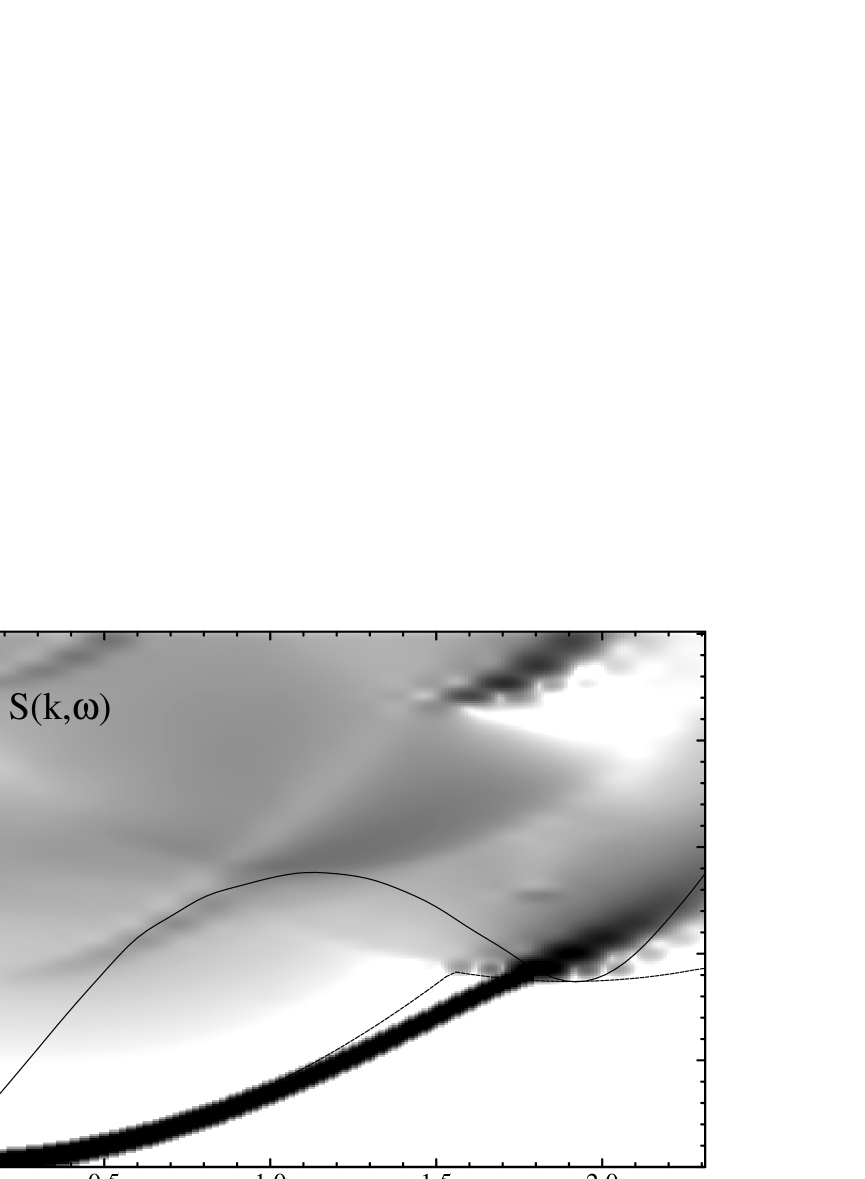
FIG. 5.: The impurity dynamic structure function $S^{(3)}(k,\omega)$ plotted in the $k,\omega$ plane. Also shown are the phonon-roton spectrum of the background ⁴He (heavy solid line, the data are from [52]), and the decay threshold of the impurity excitation mode (dashed line).

FIG. 6.: The dynamic structure function of the impurity $S^{(3)}(k,\omega)$ in the roton region as a function of $\omega$ for $k$=1.9 Å^-1, 2.1 Å^-1 and 2.3 Å^-1.

FIG. 7.: Theoretical and experimental effective mass ratio $m^{*}(P,x)\over m$ as a function of pressure $P$ and concentration $x$. The full curve is the fully self-consistent result, the dotted curve is the result without retardation effects, i.e. using the same quasiparticle interaction as in the spin–channel. The short dashed curve the static approximation. Symbols with error bars refer to the data of Ref. [28].

FIG. 8.: Same as Fig. 7 for the experiments of Ref. [29].

FIG. 9.: The figure shows a comparison between experimental (diamonds, from Fig. 1 of Ref. [39]) and theoretical magnetic susceptibilities. The vertical scale is arbitrary and taken from Ref. [39]. The theoretical results were scaled to generate the best overall fit to the data at $0.27\,\%$ and $1.33\,\%$ concentration. The solid lines are the results of the full microscopic calculation, the long dashed lines the results from using the static interaction $\tilde{W}_{\rm eff}(q)$. Note that the static results for $5.1\,\%$ concentration are close to the experiments at saturation concentration, and the static results for $8.8\,\%$ percent are off-scale.

FIG. 10.: The figure shows the calculated Landau parameter $F_{0}^{\rm a}$ determined from the microscopic interactions $\tilde{V}_{\rm eff}(q,0)$ (solid lines) and $\tilde{W}_{\rm eff}(q)$ (dashed lines) together with the results of Ahonen et al. (boxes). The highest theoretical curves correspond to zero pressure and the lowest to 20 atm. Also shown are estimates for the Landau parameter $F_{0}^{\rm a}$ from the data of Ref. [39], using the effective masses from Ref. [28] (diamonds). The lowest set of symbols corresponds to saturation pressure, the medium set to $p=10~{}$atm, and the upper set to $p=20~{}$atm. There is no experimental value at zero pressure and 8.8% concentration.

FIG. 11.: The figure shows the coordinate–space effective interactions $V_{\rm eff}(r,0)$ (solid lines) and $W_{\rm eff}(r)$ (dashed lines) for densities $\rho=0.020~{}{\rm\AA}^{-3}$ below saturation, $\rho=0.022~{}{\rm\AA}^{-3}$ close to saturation density, and $\rho=0.026~{}{\rm\AA}^{-3}$ close to solidification. The potentials with the higher repulsive peaks and deeper attractive wells correspond to the higher pressure. The Aziz–potential [3] is shown for reference (dotted line).

FIG. 12.: The figure shows the coordinate–space effective interactions $V_{\rm scat}(r)$ entering the scattering equation (83) at the density $\rho=0.022\,{\rm\AA}^{-3}$ (solid line), $\rho=0.024\,{\rm\AA}^{-3}$ (long-dashed line) and $\rho=0.026\,{\rm\AA}^{-3}$ (short-dashed line). The Aziz–potential [3] is shown for reference (dotted line).

FIG. 13.: The ³He –³He scattering phase–shifts are shown at 1 percent concentration for the densities $\rho=0.022~{}{\rm\AA}^{-3}$ (solid line), $\rho=0.024~{}{\rm\AA}^{-3}$ (long-dashed line), and $\rho=0.026~{}{\rm\AA}^{-3}$ (short-dashed line) for $\ell=0,\,1$, and $2$.

FIG. 14.: The ³He –³He scattering amplitudes corresponding to the phase shifts shown in Fig. (13) at 1 percent concentration for the densities $\rho=0.022~{}{\rm\AA}^{-3}$ (solid line), $\rho=0.024~{}{\rm\AA}^{-3}$ (long-dashed line), and $\rho=0.026~{}{\rm\AA}^{-3}$ (short-dashed line) for $\ell=0,\,1$, and $2$. The stars show the results in the simple HNC/0 approximation used by Owen [48].

FIG. 15.: The transition temperatures for $s$–wave (solid lines) and $p$–wave (dashed lines) pairing for the densities $\rho=0.022~{}{\rm\AA}^{-3}$ (upper curves) and $\rho=0.024~{}{\rm\AA}^{-3}$ (lower curves).

REFERENCES

- [1] R. de Bruyn Ouboter and C. N. Yang, Physica 144B, 127 (1986).
- [2] E. Krotscheck and M. Saarela, Phys. Rep. 232, 1 (1993).
- [3] R. A. Aziz et al., J. Chem. Phys. 70, 4330 (1979).
- [4] M. Saarela and E. Krotscheck, J. Low Temp. Phys. 90, 415 (1993).
- [5] E. Feenberg, Theory of Quantum Liquids (Academic, New York, 1969).
- [6] C. E. Campbell, in Progress in Liquid Physics, edited by C. A. Croxton (Wiley, London, 1977), Chap. 6, pp. 213–308.
- [7] C. E. Campbell and E. Feenberg, Phys. Rev. 188, 396 (1969).
- [8] C. E. Campbell, Phys. Lett. A 44, 471 (1973).
- [9] E. Krotscheck, Phys. Rev. B 33, 3158 (1986).
- [10] M. Saarela, in Recent Progress in Many Body Theories, edited by Y. Avishai (Plenum, New York, 1990), Vol. 2, pp. 337–346.
- [11] A. L. Fetter and J. D. Walecka, Quantum Theory of Many-Particle Systems (McGraw-Hill, New York, 1971).
- [12] J. C. Owen, Phys. Rev. B 23, 5815 (1981).
- [13] L. D. Landau and I. Pomeranchuk, Dokl. Akad. Nauk. SSSR 59, 669 (1948).
- [14] E. P. Bashkin and A. E. Meyerovich, Advan. Phys. 30, 1 (1981).
- [15] J. Bardeen, G. Baym, and D. Pines, Phys. Rev. Lett. 17, 372 (1966).
- [16] J. Bardeen, G. Baym, and D. Pines, Phys. Rev. 156, 207 (1967).
- [17] G. Baym and C. Pethick, Landau Fermi Liquid Theory (Wiley, New York, 1991).
- [18] E. Krotscheck and J. W. Clark, Nucl. Phys. A 328, 73 (1979).
- [19] E. Krotscheck, R. A. Smith, J. W. Clark, and R. M. Panoff, Phys. Rev. B 24, 6383 (1981).
- [20] S. Fantoni, V. R. Pandharipande, and K. E. Schmidt, Phys. Rev. Lett. 48, 878 (1982).
- [21] J. C. Wheatley, Rev. Mod. Phys. 47, 415 (1975).
- [22] T. A. Alvesalo, T. Haavasoja, M. T. Manninen, and A. T. Soinne, Phys. Rev. Lett 44, 1076 (1980).
- [23] E. Krotscheck, Phys. Rev. A 26, 3536 (1982).
- [24] L. Hedin, Phys. Rev. A 139, 796 (1965).
- [25] T. M. Rice, Ann. Phys. (NY) 31, 100 (1965).
- [26] A. D. Jackson, A. Lande, and R. A. Smith, Phys. Rep. 86, 55 (1982).
- [27] A. D. Jackson, A. Lande, and R. A. Smith, Phys. Rev. Lett. 54, 1469 (1985).
- [28] S. Yorozu, H. Fukuyama, and H. Ishimoto, Phys. Rev. B 48, 9660 (1993).
- [29] R. Simons and R. M. Mueller, Czekoslowak Journal of Physics Suppl. 46, 201 (1996).
- [30] B. Fåk et al., Phys. Rev. B 41, 8732 (1990).
- [31] A. Fabrocini and A. Polls, 1998, preprint.
- [32] D. S. Greywall, Phys. Rev. B 20, 2643 (1979).
- [33] J. R. Owers-Bradley et al., J. Low Temp. Phys. 72, 201 (1988).
- [34] H. W. Jackson, Phys. Rev. A 9, 964 (1974).
- [35] J. Harms and P. Toennies, 1998, (private communication).
- [36] S. A. Chin and E. Krotscheck, Phys. Rev. B 52, 10405 (1995).
- [37] E. Krotscheck and R. Zillich, Scattering of 3He Atoms from 4He Surfaces, 1998, submitted.
- [38] W. Hsu and D. Pines, J. Stat. Phys. 38, 273 (1985).
- [39] A. I. Ahonen, M. A. Paalanen, R. C. Richardson, and Y. Takano, J. Low Temp. Phys. 25, 733 (1976).
- [40] Y. Disatnik and H. Brucker, J. Low Temp. Phys. 7, 491 (1972).
- [41] A. Rodrigues and G. Vermeulen, J. Low Temp. Phys. 108, 103 (1997).
- [42] D. O. Edwards and S. M. Pettersen, J. Low Temp. Phys. 87, 473 (1992).
- [43] C. Ebner and D. O. Edwards, Phys. Rep. 2, 77 (1971).
- [44] C. H. Aldrich and D. Pines, J. Low Temp. Phys. 25, 677 (1976).
- [45] H. Ishimoto et al., J. Low Temp. Phys. 77, 133 (1989), (experimental; no superfluidity above 212myK).
- [46] G.-H. Oh et al., J. Low Temp. Phys. 95, 525 (1994).
- [47] R. König, A. Betat, and F. Pobell, J. Low Temp. Phys. 97, 311 (1994).
- [48] J. C. Owen, Phys. Rev. Lett. 47, 586 (1981).
- [49] S. Yorozu et al., Phys. Rev. B 45, 12942 (1992).
- [50] S. Babu and G. E. Brown, Ann. Phys. (NY) 78, 1 (1973).
- [51] E. Krotscheck, M. Saarela, K. Schörkhuber, and R. Zillich, Phys. Rev. Lett (1997), in press.
- [52] R. A. Cowley and A. D. B. Woods, Can. J. Phys. 49, 177 (1971).