On the exciton binding energy in a quantum well

Abstract

We consider a model describing the one-dimensional confinement of an exciton in a symmetrical, rectangular quantum-well structure and derive upper and lower bounds for the binding energy $E_{b}$ of the exciton. Based on these bounds, we study the dependence of $E_{b}$ on the width of the confining potential with a higher accuracy than previous reports. For an infinitely deep potential the binding energy varies as expected from $1\,Ry$ at large widths to $4\,Ry$ at small widths. For a finite potential, but without consideration of a mass mismatch or a dielectric mismatch, we substantiate earlier results that the binding energy approaches the value $1\,Ry$ for both small and large widths, having a characteristic peak for some intermediate size of the slab. Taking the mismatch into account, this result will in general no longer be true. For the specific case of a $Ga_{1-x}Al_{x}As/GaAs/Ga_{1-x}Al_{x}As$ quantum-well structure, however, and in contrast to previous findings, the peak structure is shown to survive.

I Introduction and statement of the problem

The study of electronic and excitonic properties in quantum well structures has been a subject of great interest since the pioneering work of Dingle, Wiegmann and Henry [2]. In view of the enormous amount of literature in this field, any list of references must be incomplete. We quote the publications [3, 4, 5, 6, 7, 8, 9, 10, 11, 12, 13], which are in part related to this work, and recommend the references therein. One of the most appealing features of these systems is the enhancement of excitonic effects, for instance the increase of the binding energy and the oscillator strength, which may allow the observation of an exciton even up to room temperature.

The main reason for the large binding energies and oscillator strengths is understood to be the quantum confinement of electron and hole in the growth direction of the heterostructure; in comparison to a three-dimensional monostructure, the electron-hole correlation is increased. Moreover, the mass mismatch as well as the dielectric mismatch in a quantum well may even enhance this effect, as was primarily pointed out by Keldysh[14].

In contrast to the simple qualitative reasonings, a quantitative theoretical description of the excitonic enhancement is quite complicated. The reasons are obvious; as translation symmetry is broken in the growth direction of the heterostructure, the familiar separation of center-of-mass and relative part of the exciton motion is no longer possible. If a dielectric mismatch is to be included, the electron-hole potential is no longer a simple Coulomb potential. If a mass mismatch exists, the kinetic-energy part of the Hamiltonian is no longer isotropic. Turning to real substances such as $Ga_{1-x}Al_{x}As/GaAs/Ga_{1-x}Al_{x}As$, band-structure complications (e.g. valence-band degeneracy) do occur. Moreover, the growing process may induce an interface roughness etc.. As a consequence, the spectra of excitons in a quantum well are far from being understood on a quantitative scale and different aspects have been controversially discussed in the literature.

In this paper we are concerned with one of the problems which — to the best of our knowledge — has not been solved; i.e. the position of the peak of the excitonic binding energy as a function of the width of the confining potential. Some introductory comments may be appropriate. For an infinitely deep well, the binding energy is known to vary monotonically from $1\,Ry$ to $4\,Ry$ if the width $L$ varies from infinity to zero. Contrasting this case with that of a finite well in an otherwise homogeneous material, the binding energy behaves similarly for sufficiently large values of $L$, but qualitatively different for small $L$. In the latter case, the wave function spills increasingly over the interfaces and into the barriers, occupying a greater three-dimensional volume as tunneling becomes more and more important. In the ultimate limit of zero width, the binding energy will again be $1\,Ry$. For a finite well width the confinement will increase the binding energy $E_{b}$ above $1\,Ry$. Thus we are lead to conclude that $E_{b}$ should have a maximum for some intermediate well width. In fact, this behavior was found in a variational treatment due to Greene, Bajaj, and Phelps [8]. In Sec. IV, we complement their results by lower bounds for the binding energy, which have a relative deviation of (at most) $0.2$ from the corresponding upper bounds and, furthermore, a similar shape.

A finite well in an otherwise homogeneous material should probably be viewed as a rather poor model for a real quantum well. We anticipate, however, that such a conclusion might be somewhat pessimistic. The model is well applicable as starting point for a quantitative description, but we include mismatches for the masses and the dielectric constants. What about the binding energy under these circumstances? The situation is clear in the limiting cases; for infinite well width, we start with $1\,Ry$ of the well material, whereas for zero well width, we arrive at $1\,Ry^{\prime}$ of the barrier material. Whether or not a peak appears will be sensitive to the value of $Ry/Ry^{\prime}$. Andreani and Pasquarello [9] performed a study for $Ga_{1-x}Al_{x}As/GaAs/Ga_{1-x}Al_{x}As$, including the effects of, firstly, a dielectric mismatch and, secondly, the valence band degeneracy. They did not find a peak for $x>0.25$ and a width $L>30\,\AA$, even when the band degeneracy is (theoretically) switched off.

The intention of this paper is to critically reexamine this conclusion. Clearly, our model must also resort to simplifications, as was indicated above. For each part of the heterostructure, we assume nondegenerate, isotropic and parabolic bands, but include a mass mismatch and a dielectric mismatch at the interfaces. The confinement of electron and hole is mimicked by finite rectangular wells. Our strategy is to produce upper and lower bounds for the correct binding energy of the model. Consequently, we can estimate the error of our results quantitatively. Inserting the material parameters of $Ga_{1-x}Al_{x}As/GaAs/Ga_{1-x}Al_{x}As$, $x$ varying from 0.15 to 0.40, we do find a peak structure. We can thereby disprove the above assertions.

II Formulation of the Model

To begin with, we fix the geometry of the quantum well as shown in Fig. 1. The figure shows a cut perpendicular to the $y$-axis, the well extending from $z=-L/2$ to $z=L/2$. The remaining space $|z|>L/2$ is occupied by the barrier material. The material parameters of well and barrier are denoted by unprimed and primed characters, respectively. To achieve a compact nomenclature, we define $z$-dependent expressions, e.g.

$$m(z):=m{\theta}(L/2-|z|)+m^{\prime}{\theta}(|z|-L/2),$$ (1)

for the mass of a particle; $\theta(z)$ is the familiar step function. As indicated in the figure, we assume translational invariance within the $x$-$y$ plane; consequently, the corresponding components of the total momentum are conserved.

To set up a model Hamiltonian, we proceed as described before. Introducing center-of-mass and relative coordinates for the motion in the $x$-$y$ plane, the corresponding center of mass part can be eliminated by projection on the subspace of total momentum zero. We are left with the Hamiltonian

$$H := {(2{\mu}_{\perp}(z_{e},z_{h}))}^{-1}\vec{p}_{\perp}^{\,2}+p_{z,e}{(2{m_{e}}(z_{e}))}^{-1}p_{z,e}+p_{z,h}{(2{m_{h}}(z_{h}))}^{-1}p_{z,h}$$ (3)

$$+V_{e}(z_{e})+V_{h}(z_{h})+V_{eh}(\vec{r}_{\perp},z_{e},z_{h}).$$

Here, the indices $e,h$ characterize electron and hole, respectively; $z_{e}$, $z_{h}$, $p_{z,e}$, and $p_{z,h}$ are the $z$-components of position and momentum, ${m_{e}}(z)$ and ${m_{h}}(z)$ the corresponding masses. For the relative coordinate in the $x$-$y$ plane we use the notation $\vec{r}_{\perp}:=\vec{r}_{\perp,e}-\vec{r}_{\perp,h}$, $\vec{p}_{\perp}$ denotes the corresponding momentum, and

$$({\mu}_{\perp}(z_{e},z_{h}))^{-1}:=(m_{\perp,e}(z_{e}))^{-1}+(m_{\perp,h}(z_{h}))^{-1}$$ (4)

is a generalized reduced mass. The confining potentials for electron and hole are $V_{e}(z_{e})$ and $V_{h}(z_{h})$. These potentials are assumed to be finite rectangular wells of the width $L$:

$$\displaystyle V_{i}(z_{i}):=\left\{\begin{array}[]{rcc}0,&\mbox{if}&|z_{i}|\leq L/2\ ,\\ V_{i},&\mbox{if}&|z_{i}|\geq L/2\ ,\end{array}\right.$$ (7)

where $i=e,h$. Finally, we have to specify $V_{eh}(\vec{r}_{\perp},z_{e},z_{h})$, that is the potential energy of electron and hole. To do so, we apply Poisson’s equation to find the electrostatic potential of one of the point charges (e.g. that of the hole) under the geometrical conditions of Fig. 1. At the interfaces, the familiar continuity conditions of electrodynamics have to be fulfilled. If we assume this potential to be known, its product with the electron charge yields the potential energy of interest. We note that the required solution of Poisson’s equation can conveniently be set up as follows. At first, one performs a Fourier transform of the potential with respect to the coordinates $x$ and $y$. One will realize that the remaining differential equation with respect to $z$ can be treated directly (the solutions are exponentials). In fact, this is the method, which was used by Fomin and Pokatilov [11] under more general circumstances. For the present geometry, their formulae can be somewhat simplified, leading to an explicit result for the potential energy which can be found in a paper of Kumagai and Tagakahara [12]. These authors use the method of image-charges and arrive at a power-series expansion of $V_{eh}$, the expansion parameter being

$$q:={\varepsilon-\varepsilon^{\prime}\over\varepsilon+\varepsilon^{\prime}}.$$ (8)

The zero’th order term $V_{eh}^{(0)}$ of the power series is the familiar Coulomb expression

$$V_{eh}^{(0)}(\vec{r}_{\perp},z_{e},z_{h}):=-{\bar{e}^{2}\over{\varepsilon{\,r}}},$$ (9)

the dielectric constant being that of the well material and $\bar{e}$ denotes the electron charge, divided by $\sqrt{4\pi{\varepsilon}_{0}}$ (SI units). The higher-order terms constitute the so-called image potential. For further use, we note the $q$-linear contribution explicitly:

$$V_{eh}^{(1)}(\vec{r}_{\perp},z_{e},z_{h}):=-{q\bar{e}^{2}\over\varepsilon}\left(\frac{{\Theta}_{\gg}+{\Theta}_{\ll}}{r}+\frac{1-{\Theta}_{\gg}}{r_{-}}+\frac{1-{\Theta}_{\ll}}{r_{+}}\right).$$ (10)

In this equation, we defined the distances $r$, $r_{\pm}$ and the ${\Theta}$-factors as follows:

$$r := \sqrt{r_{\perp}^{\,2}+(z_{e}-z_{h})^{2}},$$ (11)

$$r_{\pm} := \sqrt{r_{\perp}^{\,2}+(z_{e}+z_{h}\pm L)^{2}},$$ (12)

and

$${\Theta}_{\gg} := {\theta}(z_{e}-L/2)+{\theta}(z_{h}-L/2),$$ (13)

$${\Theta}_{\ll} := {\theta}(-z_{e}-L/2)+{\theta}(-z_{h}-L/2).$$ (14)

We add three remarks concerning these formulae.

The reader will notice that all terms of $V_{eh}^{(1)}$ are of Coulomb type, the corresponding denominators being partially displaced. It is important to realize that this property remains valid for all higher-order contributions (again, see Ref. [12]). Consequently, we induce an error of order $q^{2}$, if we replace the full expression for $V_{eh}$ by $V_{eh}^{(0)}+V_{eh}^{(1)}$. As $q$ is typically of the order 0.1, this simplification is reasonable and will be used in the remainder of this paper.

The second remark is concerned with an ambiguity in the power-series expansion of $V_{eh}$. Because of Eq. (8), we may replace $\varepsilon$ by ${\varepsilon^{\prime}}(1+q)/(1-q)$. Inserting this equality into Eqs. (9) and (10), we find terms of zero’th and first order as follows:

$$\tilde{V}_{eh}^{(0)}(\vec{r}_{\perp},z_{e},z_{h}):=-{\bar{e}^{2}\over{\varepsilon^{\prime}r}},$$ (15)

$$\tilde{V}_{eh}^{(1)}(\vec{r}_{\perp},z_{e},z_{h}):=-{q\bar{e}^{2}\over\varepsilon^{\prime}}\left(\frac{{\Theta}_{\gg}+{\Theta}_{\ll}-2}{r}+\frac{1-{\Theta}_{\gg}}{r_{-}}+\frac{1-{\Theta}_{\ll}}{r_{+}}\right).$$ (16)

These expansions are clearly equivalent, and will be used to our advantage in the next section.

Finally, we mention that some authors (see, e.g., Refs. [9, 12, 13]) include self-energy terms in $H$, which are also due to a dielectric mismatch. Formally these appear if one considers an electron- and a hole-inhomogeneity in Poisson’s equation and inserts the total electrostatic energy into $H$. The interaction part of this energy is the one we used above (i.e. $V_{eh}(\vec{r}_{\perp},z_{e},z_{h})$), the diagonal parts produce the self-energy terms $\Sigma(z_{e})$ for the electron (i.e. $-V_{eh}(0,z_{e},z_{e})/2$, evaluated for $\vec{r}_{\perp}=0$ and $z_{h}=z_{e}$, the bulk Coulomb singularity being subtracted) and $\Sigma(z_{h})$ for the hole. Inspection of Eq. (10) shows that $\Sigma(z)$ consists of one-dimensional Coulomb potentials, which exhibit a singularity on the interfaces $z=+L/2$ and $z=-L/2$ and vanish if $q$ vanishes. Summarizing, the confinement potentials are claimed to be changed. We doubt that modifications of the confinement potentials can be motivated this way and refer to the early quantum-mechanical debate on the hydrogen problem with (or without) self-energy corrections (e.g. Tomonaga [15]). Consequently, we did not include such corrections here. We agree, however, with the statement made in Ref. [13] that a correct microscopic description of an exciton in a quantum well should contain (well behaved) polarization-induced modifications of the rectangular confinement potentials. It should be mentioned that if we modify the confinement potentials in the way indicated above, then the corrections to the final binding energies presented in Sec. IV only appear in the vicinity of the peak being not larger than 0.5 meV.

It will prove useful to introduce dimensionless variables. For the excitonic system under consideration, appropriate units of length and energy are Bohr radius and Rydberg energy. Considering the well material, these are

$$a_{B}:={\hbar^{2}\varepsilon\over\mu_{\perp}\bar{e}^{2}},\quad Ry:={\mu_{\perp}\bar{e}^{4}\over 2\varepsilon^{2}\hbar^{2}}.$$ (17)

Returning to Eqs. (3), (9), (10), we replace $\vec{r}$ by $a_{B}\vec{r}$, introduce the dimensionless Hamiltonian

$$h:=H/Ry$$ (18)

and find the expression

$$h = -{\mu_{\perp}\over\mu_{\perp}(z_{e},z_{h})}{\vec{\nabla}}_{\perp}^{2}-{\partial\over\partial z_{e}}{\mu_{\perp}\over{m_{e}}(z_{e})}{\partial\over\partial z_{e}}-{\partial\over\partial z_{h}}{\mu_{\perp}\over{m_{h}}(z_{h})}{\partial\over\partial z_{h}}$$ (21)

$$-{2\over r}-2q\left(\frac{{\Theta}_{\gg}+{\Theta}_{\ll}}{r}+\frac{1-{\Theta}_{\gg}}{r_{-}}+\frac{1-{\Theta}_{\ll}}{r_{+}}\right)$$

$$+U_{e}(z_{e})+U_{h}(z_{h}).$$

All variables are now dimensionless. The confinement potentials read as follows;

$$\displaystyle U_{i}(z_{i}):=\left\{\begin{array}[]{rcc}0,&\mbox{if}&|z_{i}|\leq l/2,\\ U_{i},&\mbox{if}&|z_{i}|\geq l/2,\end{array}\right.$$ (24)

where we introduced

$$U_{i}:={V_{i}\over Ry},\quad l:={L\over a_{B}}.$$ (25)

The theta factors are defined as in Eq. (13) with the exception that $L$ is replaced by $l$.

We shall need a second dimensionless version of Hamiltonian (3), which is based on the Bohr radius $a_{B}^{\prime}$ and the Rydberg energy $Ry^{\prime}$ of the barrier material as well as the formulae (15), (16) for the electron-hole potential energy. Introducing

$$h^{\prime}:=H/Ry^{\prime}\ \,$$ (26)

one arrives at

$$h^{\prime} = -{\mu_{\perp}^{\prime}\over\mu_{\perp}(z_{e},z_{h})}{\vec{\nabla}}_{\perp}^{2}-{\partial\over\partial z_{e}}{\mu_{\perp}^{\prime}\over{m_{e}}(z_{e})}{\partial\over\partial z_{e}}-{\partial\over\partial z_{h}}{\mu_{\perp}^{\prime}\over{m_{h}}(z_{h})}{\partial\over\partial z_{h}}$$ (29)

$$-{2\over r}-2q\left(\frac{{\Theta}_{\gg}^{\prime}+{\Theta}_{\ll}^{\prime}-2}{r}+\frac{1-{\Theta}_{\gg}^{\prime}}{r_{-}}+\frac{1-{\Theta}_{\ll}^{\prime}}{r_{+}}\right)$$

$$+U_{e}^{\prime}(z_{e})+U_{h}^{\prime}(z_{h}).$$

The theta factors are defined as in Eq. (13) with the exception that $L$ has to be replaced by $l^{\prime}:=L/a_{b}^{\prime}$. In analogy, the confinement potentials $U^{\prime}$ can be taken from Eqs. (24) and (25), if one replaces the unprimed material parameters by primed ones.

III Upper and lower bounds for the exciton binding energy

Because of the absence of translation symmetry, the Hamiltonian $H$ (or $h$, $h^{\prime}$, respectively) cannot be treated analytically. Nevertheless, we can fix quantitative properties of the binding energy $E_{b}$ by means of rigorous bounds, which will be derived in the following sections. Our strategy will be to discuss firstly the ground-state energy $E_{0}$. The reason is that we can directly prove bounds for $E_{0}$. The binding energy $E_{b}$, in turn, is related to $E_{0}$ by the equation

$$E_{b}=E_{cont}-E_{0},$$ (30)

where $E_{cont}$ denotes the energy of the continuum edge. In our case, $E_{cont}$ is the sum of the lowest well energies of electron and hole, any correlation being neglected. For further use we note the explicit formulae

$$E_{cont}/Ry=e_{0,e}+e_{0,h},$$ (31)

where $e_{0,i}\ (i=e,h)$ is the ground-state eigenvalue of the one-dimensional well Hamiltonian

$$h_{i}:=-{\partial\over\partial z}{\mu_{\perp}\over{m_{i}}(z)}{\partial\over\partial z}+U_{i}(z),$$ (32)

part of the total Hamiltonian (21). The eigenvalue $e_{0,i}$ is implicitly defined by the equation

$$e_{0,i}={4\mu_{\perp}\over m_{i}\,l^{2}}\arcsin^{2}{\sqrt{1-e_{0,i}/U_{i}}\over\sqrt{1+({m^{\prime}_{i}}/{m_{i}}-1)e_{0,i}/U_{i}}}.$$ (33)

Due to Eq. (30), an upper (lower) bound for $E_{0}$ yields a lower (upper) bound for $E_{b}$.

A Lower bounds for the binding energy

We use a variational approach, to derive an upper bound on $E_{0}$. The trial wave function is

$$\Psi_{\alpha,\lambda}(\vec{r}_{\perp},z_{e},z_{h}):=\Phi_{e}(z_{e})\Phi_{h}(z_{h})e^{-\alpha\sqrt{r_{\perp}^{2}+\lambda z^{2}}}\hfill,$$ (34)

where $z:=z_{e}-z_{h}$ and $\Phi_{i}\ (i=e,h)$ is the ground-state eigenfunction of $h_{i}$ (see Eq. (32)). Clearly, the factors $\Phi_{e}$ and $\Phi_{h}$ serve to incorporate the single-particle well behavior.

Choosing an exponential envelope in Eq. (34), we account for two important aspects. Firstly, the confinement-induced change of the effective Bohr radius (parameter $\alpha$), and, secondly, the quenching of the wave function in $z$-direction (parameter $\lambda$). Both aspects are particularly important if one approaches the quasi two-dimensional case, where the width of the layer becomes considerably smaller than the Bohr radius of the exciton. We remark that the envelope can correctly reproduce the ultimate limits of a free exciton ground-state in two or three dimensions. Subsequently, the trial function is quite flexible and we expect the variational inequality

$${E_{0}\over Ry}\leq\min_{\lambda,\alpha}{<\Psi_{\alpha,\lambda}|h|\Psi_{\alpha,\lambda}>\over<\Psi_{\alpha,\lambda}|\Psi_{\alpha,\lambda}>}$$ (35)

to be effective. For the binding energy $E_{b}$ we derive

$${E_{b}\over Ry}\geq e_{0,e}+e_{0,h}-\min_{\lambda,\alpha}{<\Psi_{\alpha,\lambda}|h|\Psi_{\alpha,\lambda}>\over<\Psi_{\alpha,\lambda}|\Psi_{\alpha,\lambda}>}.$$ (36)

Note that the minimum of the right-hand side can be calculated for $q=0$, as we have linearized $h$ with respect to $q$.

B Upper bounds for the binding energy

In this subsection, we provide a class of lower bounds for $E_{0}$. To do so, we assume that the barrier masses $m_{e}^{\prime},m_{h}^{\prime}$ are not smaller than the corresponding well masses $m_{e},m_{h}$. This is the case for $Ga_{1-x}Al_{x}As/GaAs/Ga_{1-x}Al_{x}As$, which will be used as an example. Recalling formula (29) for the Hamiltonian under consideration, one verifies by direct inspection that the following inequality is true in the sense of operators:

$$h^{\prime}\geq\bar{h^{\prime}},$$ (37)

where

$$\bar{h^{\prime}} = :-{\vec{\nabla}}_{\perp}^{2}-{\mu_{\perp}^{\prime}\over m_{e}^{\prime}}{\partial^{2}\over\partial z_{e}^{2}}-{\mu_{\perp}^{\prime}\over m_{h}^{\prime}}{\partial^{2}\over\partial z_{h}^{2}}$$ (39)

$$-{2\over r}-2q\left(\frac{1}{r_{-}}+\frac{1}{r_{+}}\right)+U_{e}^{\prime}(z_{e})+U_{h}^{\prime}(z_{h}).$$

We stress that the above assumption $m_{i}^{\prime}\geq m_{i}$ is not crucial. If the contrary was true, we would find an analogous inequality with respect to Hamiltonian (21).

To provide a lower bound to the spectrum of $\bar{h^{\prime}}$, we split the Hamiltonian (39) into four tractable parts. Assuming the corresponding ground-state energies to be known, their sum will be a lower bound to $E_{0}/Ry^{\prime}$. Let us consider the following decomposition:

$$\bar{h^{\prime}} = h^{\prime}_{e}+h^{\prime}_{h}+h^{\prime}_{c}+h^{\prime}_{im},$$ (40)

$$h^{\prime}_{i} = :-(1-x_{i}){\mu_{\perp}^{\prime}\over m_{i}^{\prime}}{\partial^{2}\over\partial z_{i}^{2}}+U^{\prime}_{i}(z_{i}),\qquad i=e,h,$$ (41)

$$h^{\prime}_{c} = :-y{\vec{\nabla}}_{\perp}^{\,2}-x_{e}y_{e}{\mu_{\perp}^{\prime}\over m_{e}^{\prime}}{\partial^{2}\over\partial z_{e}^{2}}-x_{h}y_{h}{\mu_{\perp}^{\prime}\over m_{h}^{\prime}}{\partial^{2}\over\partial z_{h}^{2}}-{2\over r},$$ (42)

$$h^{\prime}_{im} = :-(1-y){\vec{\nabla}}_{\perp}^{\,2}-x_{e}(1-y_{e}){\mu_{\perp}^{\prime}\over m_{e}^{\prime}}{\partial^{2}\over\partial z_{e}^{2}}$$ (44)

$$-x_{h}(1-y_{h}){\mu_{\perp}^{\prime}\over m_{h}^{\prime}}{\partial^{2}\over\partial z_{h}^{2}}-2q\left(\frac{1}{r_{-}}+\frac{1}{r_{+}}\right).$$

Here, $x_{i},y_{i},y$ are parameters with values in the interval $[0,1]$ but otherwise arbitrary, which can then be chosen to lift the lower bound as much as possible. The exciton ground-state energy $E_{0}$ fulfills the inequality

$$E_{0}/Ry^{\prime}\geq e^{\prime}_{e}+e^{\prime}_{h}+e^{\prime}_{c}+e^{\prime}_{im},$$ (45)

where the four terms on the right-hand side are the ground-state eigenvalues of the four parts of $\bar{h^{\prime}}$, defined in Eq. (40). The eigenvalues $e^{\prime}_{i}$ can be derived from Eq. (33); removing the mass mismatch and rescaling the particle mass appropriately, we find

$$e^{\prime}_{i}=4(1-x_{i}){\mu_{\perp}^{\prime}\over m_{i}^{\prime}l^{\prime 2}}\arcsin^{2}\sqrt{1-e^{\prime}_{i}/U^{\prime}_{i}}.$$ (46)

Concerning $e^{\prime}_{c}$, we transform the corresponding Hamiltonian $h^{\prime}_{c}$; introducing center-of-mass and relative coordinates instead of $z_{e}$ and $z_{h}$, we can separate the center-of-mass part. Performing an appropriate scaling transformation with respect to ${\vec{r}}_{\perp}$ and $z=z_{e}-z_{h}$, we arrive at the following equations;

$$e^{\prime}_{c}={1\over y}\mbox{\rm inf spec}\left\{-\vec{\nabla}^{\,2}-{2\over\sqrt{r_{\perp}^{2}+Az^{2}}}\right\}=:{1\over y}e(A),$$ (47)

where

$$A={\mu^{\prime}_{\perp}\over\mu^{\prime}_{\parallel}}\,{x_{e}y_{e}m^{\prime}_{h}+x_{h}y_{h}m^{\prime}_{e}\over y(m^{\prime}_{e}+m^{\prime}_{h})},\quad\mu^{\prime}_{\parallel}={m^{\prime}_{e}m^{\prime}_{h}\over m^{\prime}_{e}+m^{\prime}_{h}}.$$ (48)

Clearly, $e(A)$ is (in units of $Ry^{\prime}$) the ground-state energy of an anisotropic Coulomb system. Before we comment on this, we turn to the last term in inequality (45), namely $e^{\prime}_{im}$. We transform the corresponding operator $h^{\prime}_{im}$ in two steps. Firstly, we replace $z_{h}$ by $-z_{h}$, secondly, we introduce center-of-mass and relative coordinates instead of $z_{e}$ and $z_{h}$ as was done above. We find

$$e^{\prime}_{im}=\mbox{\rm inf spec}\left\{-(1-y){\vec{\nabla}}_{\perp}^{\,2}-\mu^{\prime}_{\perp}\left[{x_{e}(1-y_{e})\over m^{\prime}_{e}}+{x_{h}(1-y_{h})\over m^{\prime}_{h}}\right]{\partial^{2}\over\partial z^{2}}-2q\left[\frac{1}{R_{-}}+\frac{1}{R_{+}}\right]\right\},$$ (49)

where $R_{+}$ and $R_{-}$ are derived from $r_{+}$ and $r_{-}$ by replacing $z_{e}+z_{h}$ by the relative coordinate $z$. Splitting the right-hand side of expression (49) again into two parts, containing the terms $1/R_{-}$ and $1/R_{+}$ separately, we may shift the variable $z$ by $+l^{\prime}$ and by $-l^{\prime}$, respectively. We obtain pure Coulomb potentials in both cases. Assuming their solutions to be known, we are finally lead to the inequality

$$e^{\prime}_{im}\geq\mbox{\rm inf spec}\left\{-(1-y){\vec{\nabla}}_{\perp}^{\,2}-\mu^{\prime}_{\perp}\left[{x_{e}(1-y_{e})\over m^{\prime}_{e}}+{x_{h}(1-y_{h})\over m^{\prime}_{h}}\right]{\partial^{2}\over\partial z^{2}}-\frac{4q}{r}\right\}.$$ (50)

Performing an appropriate scaling of variables, we can reduce the right-hand side once more to the anisotropic Coulomb problem. In comparison with Eq. (47), the parameters are changed:

$$e^{\prime}_{im}\geq{4q^{2}\over 1-y}\mbox{\rm inf spec}\left\{-\vec{\nabla}^{\,2}-{2\over\sqrt{r_{\perp}^{2}+A^{\prime}z^{2}}}\right\},$$ (51)

the anisotropy parameter now being

$$A^{\prime}={\mu^{\prime}_{\perp}\over\mu^{\prime}_{\parallel}}\,{x_{e}(1-y_{e})m_{h}+x_{h}(1-y_{h})m_{e}\over(1-y)(m_{e}+m_{h})}.$$ (52)

We summarize our results for $e^{\prime}_{c}$, $e^{\prime}_{im}$, and $E_{0}/Ry^{\prime}$. To evaluate the relations (45), (47) and (51), we need an exact expression for the ground-state eigenvalue $e(A)$ of the anisotropic Coulomb problem or, at least, a corresponding lower bound. Assuming $e(A)$ to be known, the above considerations prove the following inequality:

$${E_{0}\over Ry^{\prime}}\geq\max_{x_{e},x_{h},y_{e},y_{h},y}\left[e^{\prime}_{e}+e^{\prime}_{h}+{1\over y}e(A)+{4q^{2}\over(1-y)}e(A^{\prime})\right].$$ (53)

Finally, we arrive at a result for the binding energy, which complements the relation (36);

$${E_{b}\over Ry^{\prime}}\leq-\max_{x_{e},x_{h},y_{e},y_{h},y}\left[(e^{\prime}_{e}-e_{0,e})+(e^{\prime}_{h}-e_{0,h})+{1\over y}e(A)+{4q^{2}\over(1-y)}e(A^{\prime})\right].$$ (54)

To the best of our knowledge, an exact analytical equation for $e(A)$ is not available up to now. However, involved variational calculations were performed by several authors; we refer to the paper by Gerlach and Pollmann [16], the references therein and to our brief summary in the Appendix. The optimal upper bound on $e(A)$, which is presented in Ref. [16], will be denoted as $e_{GP}(A)$. Numerical studies indicate that $e_{GP}(A)$ deviates from $e(A)$ only on a one-percent scale, although a rigorous estimate is admittedly missing. We mention that the quoted paper also contains additional lower bounds for $e(A)$ which might be used to evaluate the preceeding inequality. In this paper we shall add another lower bound (again, see the Appendix). Unfortunately, the overall quality of all these lower bounds is not sufficient. Therefore, we will usually insert the numerical approximation $e_{GP}(A)$ instead of $e(A)$.

IV Results and discussion

A Absence of mass- and dielectric mismatch

We used this simplified model to test the efficiency of the above bounds and to illustrate the dimensional aspect. The system is interesting on it’s own and was already discussed in the literature (see Refs. [5, 8]). Here, it will prove useful to understand the well-width dependence of the binding energy on a quantitative basis.

One can easily specify the general results from above for the discussion of the present case. Equalizing all primed and unprimed material parameters, we have $q=0$ and $h=h^{\prime}$. We simplify even further by assuming $m_{e}=m_{h}$, $\mu_{\perp}=\mu_{\parallel}={m_{e}}/2$, and $U_{e}^{\prime}=U_{h}^{\prime}=U$. Turning to inequality (54) and recalling its derivation, we have to choose $y_{e}=y_{h}=y=1$ (no image potential). Consequently, the anisotropy parameter (see Eq. (48)) is fixed as $A=(x_{e}+x_{h})/2$. Summarizing at this stage, we derive from relation (54):

$${E_{b}\over Ry}\leq-\max_{x_{e},x_{h}}\left[(e_{e}-e_{0,e})+(e_{h}-e_{0,h})+e(A)\right],$$ (55)

where $e_{i}$ (see Eq. (46) is now the solution of the equation

$$e_{i}={2(1-x_{i})\over l^{2}}\arcsin^{2}\sqrt{1-e_{i}/U},$$ (56)

and $e_{i,0}$ can be derived from $e_{i}$, if we let $x_{i}=0$. The eigenvalue $e(A)$ was defined in Eq. (47). We shall now treat the cases of an infinite and a finite well. They will be shown to have a qualitatively different behavior in the narrow-well regime, as indicated in the Introduction.

For the limiting case of an infinite well we can simplify the inequality (55) as follows:

$${E_{b}\over Ry}\leq-\max_{A}\left[-A{\pi^{2}\over l^{2}}+e(A)\right].$$ (57)

To proceed, we employ another inequality, namely $e(A)\geq-4/(1+3A)$, which is derived in the Appendix. In this case, we are lead to an analytical result for $E_{b}$:

$$\displaystyle{E_{b}\over Ry}\leq\left\{\begin{array}[]{rcl}\displaystyle 4,&\mbox{if}&\displaystyle l\leq{\pi\sqrt{3}\over 6}\approx 0.91,\\[11.38109pt] \displaystyle{4\pi\sqrt{3}\over 3l}-{\pi^{2}\over 3l^{2}},&\mbox{if}&0.91\leq l\leq 3.63,\\[11.38109pt] \displaystyle 1+{\pi^{2}\over l^{2}},&\mbox{if}&\displaystyle l\geq{2\pi\sqrt{3}\over 3}\approx 3.63.\end{array}\right.$$ (61)

The right-hand side of Eq. (61) is shown as dashed-dotted curve in Fig. 3. One realizes that the required two- and three-dimensional limits 4 $Ry$ and 1 $Ry$ are reproduced, if $l$ tends to $0$ and $\infty$, respectively. Unfortunately, the overall quality of this bound is rather poor. Inserting the result $e_{GP}(A)$ for $e(A)$ as indicated in the preceding section, the upper bound on $E_{b}$ is drastically lowered as shown in the figure (dashed line for $V=\infty$). In addition, Fig. 3 contains a lower bound for the binding energy (solid curve for $V=\infty$), which is based on inequality (36).

Before we discuss the results in greater detail, we consider the finite-well case. Then, the inequality (55) has to be evaluated without further simplifications. Apart from the limiting cases $l\to 0$ and $l\to\infty$, an analytical discussion is not possible. The small-width case, however, is interesting on its own. For $l\to 0$, the solution for $e_{i}$ is

$$e_{i}=U[1-Ul^{2}/(2-2x_{i})+O(l^{3})].$$ (62)

Inserting this expression in inequality (55) and utilizing $e(A)\geq-4/(1+3A)$ again, one finds the result

$$1\leq{E_{b}\over Ry}\leq 1+\sqrt{3}Ul+O(l^{2}),\quad\mbox{\rm if}\quad l\to 0,$$ (63)

which was mentioned in the abstract as well as the Introduction. For finite values of $l$, we proceed as in the numerical treatment of the infinite well. Replacing $e(A)$ by $e_{GP}(A)$, we find the upper bounds, which are shown in Fig. 3 (dashed curves). Again, the figure includes the corresponding lower bounds (solid curves).

Clearly, the most significant attribute of these curves is the appearance of a maximum of $E_{b}$ as function of the well width $L$, if the height $V$ of the well is finite. There exists a unique relation between $V$ and the position $L_{max}$ of the maximum; for larger values of $V$ $L_{max}$ becomes smaller. All curves exhibit the expected asymptotic behavior. For finite (infinite) $V$, the large-$L$ limit of the binding energy is $1\,Ry$, the small-$L$ limit $1\,Ry$ ($4\,Ry$). Last but not least, the shape of the upper and lower bound is very similar, the relative deviation not exceeding 0.2. We are sure that the deviation as such is mostly due to the inaccuracy of the upper bound on the binding energy. We recall that the lower bound for $E_{b}$ is based on a variational upper bound on the ground-state energy, whereas the upper bound needs an accurate lower bound for $E_{0}$ as input; as usual, this part of the task is the more difficult one.

B Finite rectangular quantum well in a heterostructure

In this part we apply our theory to a single-well structure, which exhibits a mismatch of both masses and dielectric parameters. As far as specific material data are concerned, we use those of $Ga_{1-x}Al_{x}As/GaAs/Ga_{1-x}Al_{x}As$. We stress, however, that a direct comparison of our results with experimental data is limited by the fact that the present theory is clearly incomplete. An obvious shortcoming is that, for example, the effects of valence-band degeneracy, spin-orbit coupling, and exchange interaction are not included. Our intention was to analyze the implications of the well structure, in particular the inability to separate the center-of-mass and relative coordinates, as accurate as possible in order to have a well-defined basis for further improvements.

For the material parameters, we refer to the tables of Landolt-Börnstein [17] and the work of Winkler [10] (see also references therein). For $GaAs$, we used $\varepsilon=12.53,\ m_{e}=0.067m_{0}$, furthermore $m_{h}=0.090m_{0},\ \mu_{\perp}=0.051m_{0},\ Ry=4.418\ \mbox{\rm meV},\ a_{B}=130.21\ \AA$ for the light hole, and $m_{h}=0.377m_{0},\ \mu_{\perp}=0.042m_{0},\ Ry=3.638\ \mbox{\rm meV},\ a_{B}=158.12\ \AA$ for the heavy hole. For $AlAs$, the corresponding parameters are $\varepsilon=10.06\,,\,\ m_{e}=0.150m_{0}\,,\,m_{h}=0.208\,(0.478)m_{0}\,,\,\mu_{\perp}=0.106\,(0.093)m_{0}\,,\,Ry=14.2\,(12.5)\ \mbox{\rm meV}\,,\,a_{B}=50.2\,(57.2)\ \AA$ for the light (heavy) hole. The material parameters for $Ga_{1-x}Al_{x}As$ are normally described by linear interpolation formulae, for instance, $\varepsilon^{\prime}=12.53(1-x)+10.06x$, with one notable exception; the difference $\Delta E_{g}$ of the gap-energies for $x=0$ and $x>0$ is fitted as[10]

$$\Delta E_{g}=(1.087x+0.438x^{2})\ {\mbox{e}V}.$$ (64)

The precise partition of $\Delta E_{g}$ on the electronic part $V_{e}$ and the hole part $V_{h}$ has been critically discussed; to the best of our knowledge, no previous general solution exists. We used the empirical relation $V_{e}=0.65\Delta E_{g}$ and $V_{h}=0.35\Delta E_{g}$ (again, see Ref. [10]), but also indicate the consequences of modification to this assumption.

We discuss now our results. To begin with, we present lower bounds for the binding energy according to relation (36). In Fig. 4 we depict the influence of the parameter mismatches on the heavy-hole (HH) exciton of $Al_{x}Ga_{1-x}As/GaAs/Al_{x}Ga_{1-x}As$ for $x=0.3$. The thin solid curve describes the hypothetical case of equal masses and dielectric constants in well and barrier; it may be viewed as a reference line. Switching on the discontinuity of the band masses only (circles), the bound for the binding energy is lowered. We are confident that this is an artifact of our variational treatment. On the one hand, the energy of the continuum edge is exact, the effects of the mass mismatch being fully incorporated; on the other hand, the variational bound on the ground-state energy is, of course, an approximation. The difference between the two underestimates the influence of the mass mismatch. Considering only a dielectric mismatch, we find the curve depicted by triangles. One realizes that the presence of image charges shifts the binding energy to higher values, and this shift remains present for a wider range of the well width. It is only for $L\gg a_{B}$ that the energy shift disappears. Finally, the thick solid line summarizes all effects. In comparison to the reference curve, the peak height and peak position is only slightly changed; in our case, we find $L_{max}\sim 60\,\AA$ and a peak height of $9.5$ meV.

Fig. 5 presents lower bounds for the binding energies of heavy- and light-hole excitons in $Al_{x}Ga_{1-x}As/GaAs/Al_{x}Ga_{1-x}As$, assuming different $Al$-concentrations $x=0.15,\ x=0.3,\ x=0.4$. The dashed (solid) curves correspond to the light-hole (heavy-hole) exciton. The lowest (highest) curve of every set belongs to the smallest (largest) value of $x$. The observed sequence can easily be explained. A higher $Al$-concentration causes a higher band-gap difference and therefore higher potential wells. In addition, the peak positions are found to decrease with increasing $Al$-concentration. Again, the reason is clear; the higher the value of $x$, the smaller the influence of the barrier. In fact, we expect to recover the trend illustrated in Fig. 3, which is indeed the case. Above all, we find a peak structure for $x>0.25$ and $L>30\,\AA$, in contrast to the assertion of Andreani and Pasquarello [9].

We mentioned above that the actual values of $V_{e}$ and $V_{h}$ are somewhat controversial. Therefore, we found it interesting to change the fraction $V_{h}/V_{e}$. In Fig. 6 we compare lower bounds for the binding energy, $V_{h}/V_{e}$ being chosen as $35/65$ (circles) and $15/85$ (triangles), respectively; the latter value was used by Greene, Bajaj and Phelps [8]. Interestingly enough, the peak position is not changed too much.

We shall now comment on the accuracy of our results. To do so, we have chosen the HH-case of $Al_{0.3}Ga_{0.7}As/GaAs/Al_{0.3}Ga_{0.7}As$ as a representative example. In Fig. 7 we contrast lower and upper bounds for the binding energy according to Eqs. (36) and (54). The shape of the curves and the peak positions are nearly the same for both bounds, the peak heights, however, differ disappointingly by a factor 1.5. Analyzing the numerical data in detail, we realized two points: i) the adapted trial function is well localized within the well for all values of $L\geq L_{max}$ and even slightly below; ii) the upper bound for the binding energy (or, equivalently, the lower bound for the ground-state energy) grossly overestimates the mismatch. If we take (i) for granted, also for the exact wave function, we can simplify the peak problem from the very beginning. If we calculate an expectation value of $h$ (see Eq. (21)) for such a wave function, we can firstly omit all $\Theta$-factors, and secondly replace all material parameters by well parameters. Then, $h$ may be replaced by $\bar{h^{\prime}}$ (see Eq. (39)) with the important modification that all parameters in $\bar{h^{\prime}}$ have to be understood as unprimed ones, namely those of the well. Calculating lower bounds in exactly the same manner as before, we find the bounds which are denoted by approximate ones (triangles). Of course, this curve has to be cut in the region of small well widths when the requirement of prevailing localization inside the well is not fulfilled any longer. One observes that the allowed channel for the exact binding energy is now considerably smaller.

Finally, Figs. 8, 9 compare experimental and theoretical results, again for $Ga_{0.7}Al_{0.3}As/GaAs/Ga_{0.7}Al_{0.3}As$. The observed peak structure is reproduced by the present theory, but the experimental binding energies are up to 1 meV larger. There are indications that this discrepancy may be caused by our simplification of the real band structure. An enhancement of the exciton binding energies due to valence band degeneracy and conduction band nonparabolicity has been found by several authors (see, e.g., Refs. [9, 21]).

V conclusions

The intention of this work was to calculate the binding energy of an exciton in a rectangular quantum well with a higher reliability as was previously to be found in the literature. In doing so, we provided upper and lower bounds for the binding energy, which have a similar shape and constitute an allowed channel for the exact binding energy which is satisfactorily small. We can conclude that the peaks of the binding energy as function of the well width are well established within our model, and for a wide parameter range. In the case of $Ga_{1-x}Al_{x}As/GaAs/Ga_{1-x}Al_{x}As$, our results revise those of Ref. [9] thereby extending the regime of “admissable” well widths to less than $30\,\AA$. From a methodological point of view, our derivation of upper bounds on the binding energy (or, equivalently, lower bounds to the ground-state energy) can be transferred to related problems.

Upper and lower bounds for the anisotropic Coulomb problem

To evaluate the expression (54) for the lower bound on the binding energy of Hamiltonian (39), we had to provide an expression for the ground-state energy $e(A)$ of the Hamiltonian

$$h_{A} := -\vec{\nabla}^{\,2}-{2\over\sqrt{r_{\perp}^{2}+Az^{2}}}$$ (65)

$$= -\vec{\nabla}^{\,2}-{2\over\sqrt{Ar^{2}+(1-A)r_{\perp}^{2}}}.$$ (66)

We shall now briefly comment on this problem. Clearly, $e(A)$ interpolates between the two- and three-dimensional limits of the hydrogen system. If $A$ is changed from $1$ to $0$, the ground-state energy $E_{A}$ varies from -1 to -4 (in Rydberg units). Therefore, it is tempting to choose a variational wave function for the ground state as follows (see Ref. [16]):

$$\psi=Ce^{-\lambda(r+ar_{\perp})},$$ (67)

where $a,\lambda$ are variational parameters. This wave function is asymptotically exact in the three- ($A\to 1,\lambda\to 1,a\to 0$) and two-dimensional ($A\to 0,\lambda a\to 2,\lambda\to 0$) limits. Calculating the expectation value of Hamiltonian (66), one finds $e(A)\leq e_{GP}(A)$, where

$$e_{GP}(A)=\min_{a}(a^{2}-1){V^{2}(A,a)\over V^{2}(1,a)-a^{2}V^{2}(0,a)/4},$$ (68)

and

$$V(x,a)=\int\limits^{\pi/2}_{0}d\theta{\sin\theta\over(1+a\sin\theta)^{2}\sqrt{\sin^{2}\theta+x\cos^{2}\theta}}.$$ (69)

For a derivation of these equations and a discussion of the quality of the bound $e_{GP}(A)$, we again refer to Ref. [16]. In Sec. IV we made repeated use of formula (68).

Interestingly enough, the same trial wave function provides us with a lower bound for $e(A)$. To demonstrate this, we start from the identity

$$-\vec{\nabla}^{\,2}\psi+V_{tr}\psi = -\lambda^{2}(1+a)^{2}\,\psi,$$ (70)

$$V_{tr} = -\left[{2\lambda\over r}+{a\lambda\over r_{\perp}}+2a\lambda^{2}\left(1-{r_{\perp}\over r}\right)\right].$$ (71)

Thus, $\psi$ is an eigenfunction of the Hamiltonian $h_{tr}=-\vec{\nabla}^{\,2}+V_{tr}$, corresponding to the eigenvalue $e_{tr}=-\lambda^{2}(1+a)^{2}$. In fact, $\psi$ is the ground-state eigenfunction of $h_{tr}$. To prove this, one should realize that i) the ground-state of $h_{tr}$ is nondegenerate for all $a$, and ii) $e_{tr}$ coincides with the ground-state energy for $a=0$; besides, the chosen $\psi$ has no zeros. We remark that $h_{tr}$ has the same two- and three-dimensional limits as $h_{A}$.

Now let $\psi_{A}$ be the exact ground-state wave function of the Hamiltonian $h_{A}$. Then we obtain

$$e(A) = \langle\psi_{A}|h_{A}|\psi_{A}\rangle$$ (72)

$$= \langle\psi_{A}|h_{tr}-{2\over\sqrt{Ar^{2}+(1-A)r_{\perp}^{2}}}-V_{tr}|\psi_{A}\rangle$$ (73)

$$\geq e_{tr}+\langle\psi_{A}|{2\lambda\over r}+{a\lambda\over r_{\perp}}+2a\lambda^{2}\left(1-{r_{\perp}\over r}\right)-{2\over\sqrt{Ar^{2}+(1-A)r_{\perp}^{2}}}|\psi_{A}\rangle$$ (74)

$$\geq e_{tr}+\langle\psi_{A}|{1\over r}\left[2\lambda+{a\lambda\over\rho}-{2\over\sqrt{A+(1-A)\rho^{2}}}\right]|\psi_{A}\rangle,$$ (75)

where we defined $\rho:=r_{\perp}/r$ and made use of $\rho\leq 1$. The right-hand side of the latter inequality (75) may be considered as a function of the variational parameters $\lambda$ and $a\lambda$ ($A$ being the experimental “input”). We evaluate this function as follows. Firstly, we calculate the minimum of the expression in square brackets as a function of $\rho$; inserting the corresponding solution into inequality (75), the square bracket is a pure $c$-number and can be extracted from the expectation value. Secondly, we choose $\lambda$ such that the extracted square bracket vanishes and, finally, $a\lambda$ such that the lower bound assumes a maximum. This leads us to

$$e(A)\geq-{4\over 1+3A}.$$ (76)

Obviously, this lower bound gives the correct values $e(1)=-1$ and $e(0)=-4$.

a                 

FIG. 1.: Geometry of the quantum well

FIG. 2.: Upper (solid lines) and lower (dashed lines) bounds for the anisotropic Coulomb problem. The solution which is considered as numerically exact is drawn as a thick line.

FIG. 3.: Binding energy as function of the well thickness for different potential heights, showing comparison of variational calculation (solid lines) and lower bound method (dashed lines). The dashed-dotted line shows the result for the simple analytical lower bound from the Appendix.

FIG. 4.: Binding energy of a HH-exciton in $Al_{0.3}Ga_{0.7}As/GaAs/Al_{0.3}Ga_{0.7}As$; the effect of dielectric and mass mismatch is shown separately by the triangle and circle symbols, respectively. The thick solid line illustrates the result of both contributions.

FIG. 5.: Binding energies of the HH- and LH-exciton for different $Al$-concentrations $x=0.15,x=0.3,x=0.4$. The variational approach including parameter mismatch is applied. The lowest (highest) curves belong to the smallest (largest) value of $x$.

FIG. 6.: Binding energies of the HH- and LH-exciton for different valence band offsets in $Al_{0.4}Ga_{0.6}As/GaAs/Al_{0.4}Ga_{0.6}As$. The valence band offsets are chosen either from Greene, Bajaj and Phelps[8] (triangles) or from Andreani and Pasquarello[9] (circles).

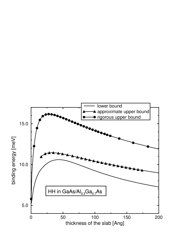
FIG. 7.: Rigorous upper bounds (circles) and lower bounds (lines) in comparison with approximate upper bounds for the exciton binding energy in $Al_{0.3}Ga_{0.7}As/GaAs/Al_{0.3}Ga_{0.7}As$.

FIG. 8.: Comparison of the present calculations (solid and dashed-dotted lines) with experimental data (stars and triangles) as well as with theoretical data (square symbols) for the heavy-hole-exciton in $Al_{0.3}Ga_{0.7}As/GaAs/Al_{0.3}Ga_{0.7}As$.

FIG. 9.: Comparison of the present calculations (solid and dashed-dotted lines) with experimental data (stars) as well as with theoretical data (square symbols) for the light-hole-exciton in $Al_{0.3}Ga_{0.7}As/GaAs/Al_{0.3}Ga_{0.7}As$.

REFERENCES

- [1] E-mail address: gerlach@fkt.physik.uni-dortmund.de
- [2] R. Dingle, W. Wiegmann, and C. H. Henry, Phys. Rev. Lett. 33, 827 (1974); see also R. Dingle, in Festkörperprobleme , ed. H. J. Queisser (Vieweg, Braunschweig, 1975); p. 21.
- [3] Confined Electrons and Photons, New Physics and Applications, eds. E. Burstein and C. Weisbuch (Plenum Press 1995).
- [4] Heterojunctions and Semiconductor Superlattices, Proceedings of the Winter School Les Houches, France 1985, eds. G. Allan, G. Bastard, N. Boccara, M. Lannoo, and M. Voos (Springer, Berlin 1986).
- [5] Optics of Excitons in Confined Systems, ed. A. D’Andrea, R. Del Sole, R. Girlanda, and A. Quattropani, Institute of Physics Conference Series No. 123.
- [6] G. Bastard, Wave Mechanics Applied to Semiconductor Heterostructures, Les editions de physique (Halsted Press 1988).
- [7] G. Bastard, E. E. Mendez, L. L. Chang, and L. Esaki, Phys. Rev. B 26, 1974 (1982).
- [8] R. L. Greene, K. K. Bajaj, and D. E. Phelps, Phys. Rev. B 29, 1807 (1984).
- [9] L. C. Andreani and A. Pasquarello, Phys Rev. B 42, 8928 (1990).
- [10] R. Winkler, Phys. Rev. B 51, 14395 (1995).
- [11] V. M. Fomin and E. P. Pokatilov, phys. stat. sol. (b) 129, 203 (1985).
- [12] M. Kumagai and T. Takagahara, Phys. Rev. B 40, 12359 (1989).
- [13] D. B. Tran Thoai, R. Zimmermann, M. Grundmann, and D. Bimberg, Phys. Rev. B 42, 5906 (1990).
- [14] L. V. Keldysh, JETP Lett. 29, 659 (1979).
- [15] S. I. Tomonaga, Quantum Mechanics, (North-Holland Publishing Company, Amsterdam 1966).
- [16] B. Gerlach and J. Pollmann, phys. stat. sol. (b) 67, 93 (1975), and Nuov. Cim. B 38, 423 (1977).
- [17] Landolt-Börnstein Numerical Data and Functional Relationships in Science and Technology, ed. O. Madelung (Springer, Berlin 1982).
- [18] M. Gurioli, J. Martinez-Pastor, M. Colocci, A. Bosacchi, S. Franchi, and L. C. Andreani, Phys. Rev B 47, 15755 (1993).
- [19] V. Voliotis, R. Grousson, P. Lavallard, and R. Planel, Phys. Rev. B 52, 10725 (1995).
- [20] C. Priester, G. Allan, and M. Lannoo, Phys. Rev. B 30, 7302 (1984).
-
[21]
G. D. Sanders and Y.-C. Chang,
Phys. Rev. B 32, 5517 (1985);
D. A. Broido and L. J. Sham, Phys. Rev. B 34, 3917 (1986);
U. Ekenberg and M. Altarelli, Phys. Rev. B 35, 7585 (1987);
G. E. W. Bauer and T. Ando, Phys. Rev. B 38, 6015 (1988).