Network Model for a 2D Disordered Electron System with Spin-Orbit Scattering

Abstract

We introduce a network model to describe two-dimensional disordered electron systems with spin-orbit scattering. The network model is defined by a discrete unitary time evolution operator. We establish by numerical transfer matrix calculations that the model exhibits a localization-delocalization transition. We determine the corresponding phase diagram in the parameter space of disorder scattering strength and spin-orbit scattering strength. Near the critical point we determine by statistical analysis a one-parameter scaling function and the critical exponent of the localization length to be $\nu=2.51\pm 0.18$. Based on a conformal mapping we also calculate the scaling exponent of the typical local density of states $\alpha_{0}=2.174\pm 0.003$.

]

I Introduction

Recently, localization-delocalization (LD) transitions in 2D disordered electron systems in the absence of a magnetic field were observed by several groups [1, 2, 3, 4, 5, 6, 7]. These results are in contrast with the scaling theory for non-interacting electrons [8], which predicts that all states are localized in two dimensions and in the absence of spin-orbit interaction (SOI). Now, a new discussion has started on this topic with the emphasis on the effects of electron-electron interaction and spin-orbit interaction [9, 10, 11, 12, 13].

It is known that both types of interactions could be responsible for the existence of a LD transition. In the case of SOI, general arguments [14] and perturbation theoretical calculations in the weakly disordered regime [15, 16] yield a positive correction to the conductance. This quantum interference effect requiring time reversal invariance is known as weak anti-localization. In the present work we focus on the detailed examination of a 2D non-interacting electron system with SOI. For these purposes we formulate a scattering theoretical network model for such a system.

In a recent paper [17] is was shown that scattering theoretical network models (NWMs) are well suited to describe mesoscopic disordered electron system. In general such a NWM can represent any system of coherent waves propagating through disordered media. It consists of a network of unitary scatterers connected by bonds. The arrangement of scatterers and bonds defines the topology of the NWM, which can be described by a connectivity matrix. In our work we have chosen a simple case, where the scatterers are located on the sites of a quadratic grid, so each of them has four nearest neighbors. Each bond consists of $2n$ links, $n$ for each direction, where $n=1$ for waves without and $n>1$ for waves with internal degrees of freedom (cf. Fig. 1). In the case of electron waves a complex number is attached to each link representing the probability amplitude at this position. The set of all amplitudes defines the quantum mechanical state $\Psi(t)$ at time $t$. One step of time evolution is then given by a unitary operator $\cal{U}$,

$$\Psi(t+1)={\cal U}\Psi(t).$$ (1)

This time evolution operator is determined by all the scatterers in the NWM. Each scatterer maps $4n$ incoming channels to $4n$ outgoing channels conserving the current and is therefore represented by a unitary $4n\times 4n$-matrix. The disorder is in general simulated in two ways: first by multiplying the amplitude on each link with a complex random phase factor ${\text{e}}^{{\text{i}}\phi}$ with $\phi$ randomly chosen from $[0,2\pi[$ simulating the random distances between the scatterers and secondly by taking random values for the parameters that parameterize the matrix representation of the scatterers simulating the random strengths of the scatterers. Of course, both random choices have to be compatible with the symmetry properties of the system. We distinguish 2D electron systems with time reversal symmetry (O2NC) and without time reversal symmetry (U2NC), both without spin degrees of freedom, and systems with time reversal symmetry and spin degrees of freedom (S2NC). The ”2” refers to the space dimension, the ”O”, ”U” and ”S” mean ”orthogonal”, ”unitary” and ”symplectic”, which refers to the corresponding universality classes of random matrix theory and the letters ”NC” indicate that all these systems are ”non-chiral”, which means that no orientation is preferred as would be in presence of a strong magnetic field.

FIG. 1.: Topology of a general network model. Squares are scatterers and lines are bonds.

The two former models have been examined extensively in [18]. In this work a reflection, a transmission and a deflection coefficient were introduced, which parameterize the scattering matrices. Furthermore an elastic mean free path was defined in terms of these coefficients. It was concluded that all states are localized in the O2NC-/U2NC-NWM.

In the present work we investigate the S2NC-NWM. We find a parameterization for the matrix representation of the spin scatterers and introduce a spin scattering strength. The calculation of the localization length by the transfer matrix method allows us to detect the LD transition and to determine the scaling function. In order to quantify the scaling exponent $\nu$ of the correlation length we use a fit procedure [19]. We fit the scaling function and the critical exponent in two steps respecting the correlations of the data. Additionally, we apply a $\chi^{2}$-test to estimate the confidence of the fits. Determining the critical value of the localization length we find the scaling exponent $\alpha_{0}$ of the typical local density of states using a conformal mapping [20].

This paper is organized as follows: In Sec. II we introduce the network model by explicitly constructing the scattering matrices. Sec. III contains the transformation to the transfer matrices and summarizes general aspects of LD transitions. A detailed description of the methods of data evaluation forms the content of Sec. IV. The discussion of the results is presented in Sec. V followed by a short summary in Sec. VI.

II Network Model

A Topology

There are two different types of scatterers in the S2NC-NWM: potential scatterers (PSs) changing only the electron’s direction and spin scatterers (SSs) changing only the electron’s spin. The network consists of a regular 2D quadratic grid of potential scatterers each of them connected to the four next neighbors by bonds. On each bond a spin scatterer is placed leaving the electron’s direction unchanged (cf. Fig. 2).

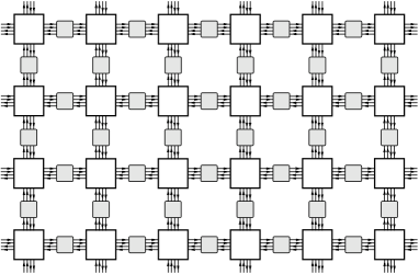
FIG. 2.: Topology of the network. The potential scatterers (white) change the direction, the spin scatterers (grey) the spin of the electrons.

B Potential scatterers

There are four channels or links within each bond, two of them for incoming and two of them for outgoing states with spin up and spin down, respectively. The electronic state is represented by complex numbers (amplitudes) on each link. Consequently, each PS maps eight incoming channels $I^{\sigma}_{i}$ to eight outgoing channels $O^{\sigma}_{i}$ ($\sigma\in\{+,-\}$, $i\in\{1,2,3,4\}$) and thus can be represented by a $8\times 8$-matrix ${\sf S}_{\text{pot}}$. With the definition of the geometrical arrangement of the channels shown in Fig. 3 this mapping is defined as follows:

$$\mathchoice{{\hbox{\boldmath$\displaystyle O$}}}{{\hbox{\boldmath$\textstyle O$}}}{{\hbox{\boldmath$\scriptstyle O$}}}{{\hbox{\boldmath$\scriptscriptstyle O$}}}={\sf S}_{\text{pot}}\mathchoice{{\hbox{\boldmath$\displaystyle I$}}}{{\hbox{\boldmath$\textstyle I$}}}{{\hbox{\boldmath$\scriptstyle I$}}}{{\hbox{\boldmath$\scriptscriptstyle I$}}}\qquad\text{with}\quad\mathchoice{{\hbox{\boldmath$\displaystyle I$}}}{{\hbox{\boldmath$\textstyle I$}}}{{\hbox{\boldmath$\scriptstyle I$}}}{{\hbox{\boldmath$\scriptscriptstyle I$}}}=\left(\begin{array}[]{c}I^{+}_{1}\\ I^{-}_{1}\\ \vdots\\ I^{+}_{4}\\ I^{-}_{4}\end{array}\right)\,,\normalsize\mathchoice{{\hbox{\boldmath$\displaystyle O$}}}{{\hbox{\boldmath$\textstyle O$}}}{{\hbox{\boldmath$\scriptstyle O$}}}{{\hbox{\boldmath$\scriptscriptstyle O$}}}=\left(\begin{array}[]{c}O^{+}_{1}\\ O^{-}_{1}\\ \vdots\\ O^{+}_{4}\\ O^{-}_{4}\end{array}\right).$$ (2)

FIG. 3.: Potential scatterer: The eight incoming channels $I_{i}^{\sigma}$ are mapped to the eight outgoing channels $O_{i}^{\sigma}$.

Due to current conservation,

$$\sum_{i,\sigma}\left|I_{i}^{\sigma}\right|^{2}=\sum_{i,\sigma}\left|O_{i}^{\sigma}\right|^{2},$$ (3)

each scattering matrix has to be unitary,

$${\sf S}_{\text{pot}}\cdot{\sf S}_{\text{pot}}^{\dagger}=\openone_{8},$$ (4)

where $\openone_{8}$ denotes the $8\times 8$ identity matrix. Additionally, the scatterers are time reversal invariant. Both properties yield the matrix to be symmetric,

$${\sf S}_{\text{pot}}={\sf S}_{\text{pot}}{{}^{\text{T}}},$$ (5)

where T denotes the transpose.

For convenience we choose the potential scatterers to be isotropic, i.e. they are invariant under rotations by multiple angles of $\pi/2$. With these restrictions each scattering matrix ${\sf S}_{\text{pot}}$ can be parameterized in the following way [18]:

$${\sf S}_{\text{pot}}=\Phi\tilde{\sf S}_{\text{pot}}\Phi$$ (6)

with

$$\tilde{\sf S}_{\text{pot}}=\left(\begin{array}[]{cccc}r{\text{e}}^{{\text{i}}\phi_{r}}&d&d&t{\text{e}}^{{\text{i}}\phi_{t}}\\ d&r{\text{e}}^{{\text{i}}\phi_{r}}&t{\text{e}}^{{\text{i}}\phi_{t}}&d\\ d&t{\text{e}}^{{\text{i}}\phi_{t}}&r{\text{e}}^{{\text{i}}\phi_{r}}&d\\ t{\text{e}}^{{\text{i}}\phi_{t}}&d&d&r{\text{e}}^{{\text{i}}\phi_{r}}\\ \end{array}\right)\otimes\openone_{2}$$ (7)

and

$$\Phi=\left(\begin{array}[]{cccc}{\text{e}}^{{\text{i}}\phi_{1}}&0&0&0\\ 0&{\text{e}}^{{\text{i}}\phi_{2}}&0&0\\ 0&0&{\text{e}}^{{\text{i}}\phi_{3}}&0\\ 0&0&0&{\text{e}}^{{\text{i}}\phi_{4}}\\ \end{array}\right)\otimes\openone_{2}.$$ (8)

Here $\openone_{2}$ denotes the $2\times 2$ identity matrix and $\otimes$ is the tensor product. The real parameters $r,t,d$ denote the reflection, transmission and deflection (right and left scattering) coefficient, respectively (cf. Fig. 4). If we choose $r$ and $t$ as independent parameters for ${\sf S}_{\text{pot}}$, the real phases $\phi_{r}$, $\phi_{t}$ and the deflection coefficient $d$ are related to them due to unitarity and time reversal symmetry,

$$\left|r\right|^{2}+2\left|d\right|^{2}+\left|t\right|^{2} = 1,$$ (10)

$$\left|r\right|\cdot\left|d\right|\cos\phi_{r} = -\left|t\right|\cdot\left|d\right|\cos\phi_{t},$$ (11)

$$\left|r\right|\cdot\left|t\right|\cos(\phi_{r}-\phi_{t}) = \left|d\right|^{2}.$$ (12)

Furthermore, two restrictions follow from these equations,

$$r^{2}+t^{2}\; \leq\;1,$$ (14)

$$r\phantom{{}^{2}}+t\phantom{{}^{2}}\; \geq\;1.$$ (15)

FIG. 4.: Definition of the reflection coefficient $r$, the transmission coefficient $t$ and the deflection coefficient $d$.

The four real phases $\phi_{1},\dots,\phi_{4}$ which are randomly chosen from the interval $[0,2\pi[$ model the spatial disorder. They can be interpreted as phase factors ${\text{e}}^{{\text{i}}\phi_{i}}$ for freely propagating electron waves. Consequently, there are six independent parameters. But only $r$ and $t$ govern the macroscopic properties of the system. For convenience we choose them to be equal for all PSs in the network, whereas the phases are randomly taken for each scatterer.

C Spin scatterers

The spin scatterers located between the potential scatterers have two incoming and two outgoing channels on the left and on the right, respectively, as is shown in Fig. 5. They can be represented by $4\times 4$-matrices ${\sf S}_{\text{sp}}$:

$$\mathchoice{{\hbox{\boldmath$\displaystyle O$}}}{{\hbox{\boldmath$\textstyle O$}}}{{\hbox{\boldmath$\scriptstyle O$}}}{{\hbox{\boldmath$\scriptscriptstyle O$}}}={\sf S}_{\text{sp}}\mathchoice{{\hbox{\boldmath$\displaystyle I$}}}{{\hbox{\boldmath$\textstyle I$}}}{{\hbox{\boldmath$\scriptstyle I$}}}{{\hbox{\boldmath$\scriptscriptstyle I$}}}\qquad\text{with}\quad\mathchoice{{\hbox{\boldmath$\displaystyle I$}}}{{\hbox{\boldmath$\textstyle I$}}}{{\hbox{\boldmath$\scriptstyle I$}}}{{\hbox{\boldmath$\scriptscriptstyle I$}}}=\left(\begin{array}[]{c}I^{+}\\ I^{-}\\ \tilde{I}^{+}\\ \tilde{I}^{-}\end{array}\right)\,,\normalsize\mathchoice{{\hbox{\boldmath$\displaystyle O$}}}{{\hbox{\boldmath$\textstyle O$}}}{{\hbox{\boldmath$\scriptstyle O$}}}{{\hbox{\boldmath$\scriptscriptstyle O$}}}=\left(\begin{array}[]{c}O^{+}\\ O^{-}\\ \tilde{O}^{+}\\ \tilde{O}^{-}\end{array}\right).$$ (16)

FIG. 5.: Spin scatterer: The four incoming channels $I^{\sigma}$, $\tilde{I}^{\sigma}$ are mapped to the eight outgoing channels $O^{\sigma}$, $\tilde{O}^{\sigma}$.

Unitarity and time reversal symmetry result in

$${\sf S}_{\text{sp}}={\sf D}^{\text{T}}{\sf S}_{\text{sp}}^{\text{T}}{\sf D}$$ (17)

and

$${\sf S}_{\text{sp}}={\sf D}^{\text{T}}K{\sf S}_{\text{sp}}^{-1}K{\sf D}={\sf D}^{\text{T}}\bigl{(}{\sf S}_{\text{sp}}^{-1}\bigr{)}^{\ast}{\sf D},$$ (18)

respectively. Here the asterisk denotes complex conjugation and $K{\sf D}$ is the time-reversal operator with complex conjugation operator $K$ and

$${\sf D}=\left(\begin{array}[]{cc}-\tau_{2}&0\\ 0&-\tau_{2}\end{array}\right)=\left(\begin{array}[]{cc}{\sf J}&0\\ 0&{\sf J}\end{array}\right)\;,$$ (19)

where $\tau_{2}$ is one of the basis quaternions $(\tau_{0},\mathchoice{{\hbox{\boldmath$\displaystyle\tau$}}}{{\hbox{\boldmath$\textstyle\tau$}}}{{\hbox{\boldmath$\scriptstyle\tau$}}}{{\hbox{\boldmath$\scriptscriptstyle\tau$}}})=(\tau_{0},\tau_{1},\tau_{2},\tau_{3})$ given by

$$\tau_{0}=\openone_{2}\quad\text{and}\quad\mathchoice{{\hbox{\boldmath$\displaystyle\tau$}}}{{\hbox{\boldmath$\textstyle\tau$}}}{{\hbox{\boldmath$\scriptstyle\tau$}}}{{\hbox{\boldmath$\scriptscriptstyle\tau$}}}=-{\text{i}}\mathchoice{{\hbox{\boldmath$\displaystyle\sigma$}}}{{\hbox{\boldmath$\textstyle\sigma$}}}{{\hbox{\boldmath$\scriptstyle\sigma$}}}{{\hbox{\boldmath$\scriptscriptstyle\sigma$}}}$$ (20)

with Pauli matrices $\mathchoice{{\hbox{\boldmath$\displaystyle\sigma$}}}{{\hbox{\boldmath$\textstyle\sigma$}}}{{\hbox{\boldmath$\scriptstyle\sigma$}}}{{\hbox{\boldmath$\scriptscriptstyle\sigma$}}}=(\sigma_{x},\sigma_{y},\sigma_{z})$. The matrix

$${\sf J}=\left(\begin{array}[]{cc}0&1\\ -1&0\end{array}\right)$$ (21)

is the symplectic unit matrix. The symmetries (17) and (18) suggest the following parameterization of the spin scattering matrix,

$${\sf S}_{\text{sp}}=\left(\begin{array}[]{cc}0&{\text{e}}^{{\text{i}}{\varphi}}q\\ {\text{e}}^{{\text{i}}{\varphi}}\bar{q}&0\end{array}\right)$$ (22)

with the quaternion real matrix

$$q=\sum_{k=0}^{3}q_{k}\tau_{k}=\left(\begin{array}[]{cc}q_{0}-{\text{i}}q_{3}&-q_{2}-{\text{i}}q_{1}\\ q_{2}-{\text{i}}q_{1}&q_{0}+{\text{i}}q_{3}\end{array}\right)\in SU(2),$$ (23)

where the real coefficients $q_{i}$ are restricted by $\sum_{k=0}^{3}q_{k}^{2}=1$ due to unitarity and $\bar{q}$ denotes the quaternion conjugation [21]. Thus, three independent parameters remain which are randomly and homogeneously taken from the unit sphere for each SS. The phase $\varphi$ is randomly taken from $[0,2\pi[$. In random matrix theory the symmetries (17) and (18) correspond to an ensemble of quaternion real Hamiltonians, which can be diagonalized by symplectic transformations. Because of this, we also refer to this symmetry as symplectic symmetry.

We now define the spin scattering strength by

$$s=\sqrt{1-q_{0}}=\sqrt{q_{1}^{2}+q_{2}^{2}+q_{3}^{2}}.$$ (24)

This quantity takes values in the interval $[0,1]$, where $s=0$ means no spin scattering and $s=1$ full spin scattering, resulting in full spin relaxation after one scattering event. The parameter $s$ is fixed for the whole network.

D Parameter space

In conclusion there are three independent quantities building up the three dimensional parameter space (or phase space) of the S2NC-NWM. With the restrictions (II B) and $s\in[0,1]$ the possible values $(r,t,s)$ are located in a certain volume in ${\mathbb{R}}^{3}$. Fig. 6 shows a cross-section of this volume at some fixed value of $s$. The grey area contains the allowed values. If the time reversal symmetry is omitted, i.e. switching to the U2NC-NWM, the phase space (at some fixed s) is the entire quarter of the circle.

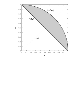
FIG. 6.: Cross-section of the parameter space at some fixed $s$.

There are three exceptional points in the phase space: For $r=0$ and $t=1$ we have the delocalized fixed point, where the electron waves propagate freely. If we take $r=1$ and $t=0$, we have the localized fixed point, where transport stops. For $r=t=0$ the network is at the Chalker-Coddington fixed point [22], where only left and right scattering exists. On the line $r^{2}+t^{2}=1$ the deflection coefficient is zero. Thus, the system splits in independent 1D subsystems which always show localization. All of these properties are independent of the value of $s$.

In [18] an elastic mean free path is defined by

$$l_{\text{e}}:=\frac{1}{2}\frac{t^{2}+d^{2}}{r^{2}+d^{2}}\;.$$ (25)

The factor $1/2$ is a consequence of the diagonal arrangement, which is shown in Fig. 7. The unit of $l_{\text{e}}$ is a lattice constant. Analogously, we define a spin scattering length by

$$l_{\text{SO}}:=\frac{1}{2}\frac{1-s^{2}}{s^{2}}\>.$$ (26)

This length scale takes values from 0 for maximal spin scattering to $\infty$ in the case of the absence of spin scattering.

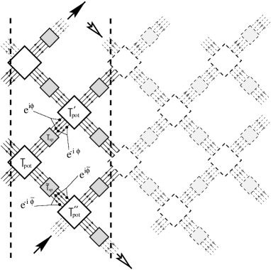
FIG. 7.: Definition of the strip transfer matrix for $M=2$. The arrows indicate the periodic boundary conditions.

III Finite-Size Scaling

A Transfer Matrix Method

In order to investigate the scaling behavior of the modeled system we need some scaling variable. Although the conductance is the natural choice for a scaling variable in this context, the renormalized localization length (RLL) $\Lambda=\xi/M$ is, as a self-averaging quantity, much more convenient. Here $\xi$ is the localization length of a quasi-1D system of width $M$ and can be calculated by the transfer matrix method [23, 24]. This method yields a sequence of Lyapunov exponents in decreasing order, where (due to conservation of current density) each value has a partner with opposite sign. Beyond this, in presence of SOI each value appears twice, because of time reversal symmetry (Kramers degeneracy). The smallest positive Lyapunov exponent determines the quasi-1D localization length. It is always finite due to the finite width of the system.

In order to be able to apply the transfer matrix method we have to convert our scattering matrices ${\sf S}_{\text{pot}}$ and ${\sf S}_{\text{sp}}$ into the corresponding transfer matrices ${\sf T}_{\text{pot}}$ and ${\sf T}_{\text{sp}}$, which map channels on the left to channels on the right. In contrast to the scattering matrices the transfer matrices are multiplicative, which means the following: The total system is divided into a sequence of elementary subsystems each of them corresponding to a single transfer step. The transfer matrix of the total system is then given by the product of the transfer matrices of the subsystems (”strip transfer matrices”).

B Transfer Matrices in the Network Model

With the channel orientation of Fig. 3 and Fig. 5 the transfer matrices of the S2NC-NWM are defined by

$$\left(\begin{array}[]{c}O^{+}_{3}\\ O^{-}_{3}\\ I^{+}_{3}\\ I^{-}_{3}\\ O^{+}_{4}\\ O^{-}_{4}\\ I^{+}_{4}\\ I^{-}_{4}\end{array}\right)={\sf T}_{\text{pot}}\left(\begin{array}[]{c}I^{+}_{1}\\ I^{-}_{1}\\ O^{+}_{1}\\ O^{-}_{1}\\ I^{+}_{2}\\ I^{-}_{2}\\ O^{+}_{2}\\ O^{-}_{2}\end{array}\right)$$ (27)

and

$$\left(\begin{array}[]{c}\tilde{O}^{+}\\ \tilde{O}^{-}\\ \tilde{I}^{+}\\ \tilde{I}^{-}\end{array}\right)={\sf T}_{\text{sp}}\left(\begin{array}[]{c}I^{+}\\ I^{-}\\ O^{+}\\ O^{-}\end{array}\right)\>,$$ (28)

respectively. From this definition a diagonal arrangement of the whole network results, as is shown in Fig. 7. The arrows at the top and the bottom of the figure indicate the periodic boundary conditions which we have chosen. The natural width unit in this arrangement is a pair of diagonally neighbored transfer matrices, which corresponds to a channel number of $N_{\text{c}}=8$. Therefore the bold printed part of the picture represents a strip transfer matrix of width $M=2$, channel number $N_{\text{c}}=16$ and unit length $L=1$ (horizontal direction).

In the language of transfer matrices the conservation of current density writes as pseudo-unitarity:

$${\sf T}_{\text{pot}}\Sigma_{z}{\sf T}_{\text{pot}}^{\dagger}=\Sigma_{z}$$ (29)

with

$$\Sigma_{z}=\left(\begin{array}[]{cc}\openone_{4}&0\\ 0&-\openone_{4}\end{array}\right)\>,$$ (30)

and

$${\sf T}_{\text{sp}}\Sigma_{z}^{\prime}{\sf T}_{\text{sp}}^{\dagger}=\Sigma_{z}^{\prime}$$ (31)

with

$$\Sigma_{z}^{\prime}=\left(\begin{array}[]{cc}\openone_{2}&0\\ 0&-\openone_{2}\end{array}\right),$$ (32)

respectively. On the other hand, time reversal invariance requires

$${\sf T}_{\text{pot}}=\left(\begin{array}[]{cc}0&{\sf D}\\ {\sf D}&0\end{array}\right)^{\text{T}}{\sf T}_{\text{pot}}^{\ast}\left(\begin{array}[]{cc}0&{\sf D}\\ {\sf D}&0\end{array}\right)$$ (33)

and

$${\sf T}_{\text{sp}}={\sf D}^{\text{T}}{\sf T}_{\text{sp}}^{\ast}{\sf D}\;,$$ (34)

with ${\sf D}$ as given in (19). A parameterization of ${\sf T}_{\text{pot}}$ compatible with these restrictions is given by [18]

$${\sf T}_{\text{pot}}=\left(\begin{array}[]{cccc}\alpha^{\ast}&\gamma&\beta^{\ast}&\delta\\ -\gamma&\alpha&-\delta&\beta\\ \beta^{\ast}&\delta&\alpha^{\ast}&\gamma\\ -\delta&\beta&-\gamma&\alpha\\ \end{array}\right)\otimes\openone_{2}$$ (35)

with

$$\begin{array}[]{ll}\displaystyle\alpha=\displaystyle\frac{d}{\Delta},&\displaystyle\beta=-\frac{t\text{e}^{\text{i}\phi_{t}}}{\Delta},\\[14.22636pt] \displaystyle\gamma=\frac{(r\text{e}^{\text{i}{\phi_{r}}}-t\text{e}^{\text{i}\phi_{t}})d}{\Delta},&\displaystyle\delta=\frac{d^{2}-r{\text{e}}^{{\text{i}}\phi_{r}}t{\text{e}}^{{\text{i}}\phi_{t}}}{\Delta},\\[14.22636pt] \Delta=d^{2}-(t{\text{e}}^{{\text{i}}\phi_{t}})^{2}.&\end{array}$$ (36)

For ${\sf T}_{\text{sp}}$ we find

$${\sf T}_{\text{sp}}=\left(\begin{array}[]{cc}{\text{e}}^{{\text{i}}{\varphi}}\bar{q}&0\\ 0&{\text{e}}^{-{\text{i}}{\varphi}}\bar{q}\end{array}\right)$$ (37)

with $\bar{q}$ as in Eq. (23). We omitted the four phase factors in ${\sf T}_{\text{pot}}$ because they can be combined with those of ${\sf T}_{\text{sp}}$ to a resulting phase factor $\varphi$ in ${\sf T}_{\text{sp}}$.

C Localization-Delocalization Transition

The scaling behavior of the RLL $\Lambda$ determines whether the system is localized or delocalized. If $\Lambda$ shrinks with increasing system width $M$ the system behaves like an insulator, if it grows, the system is metallic. At the LD transition the RLL is independent of the system width. To ensure that $\Lambda$ is in fact a scaling variable one has to find a scaling function that is a function of only the ratio of the correlation length $\xi_{\text{c}}$ and $M$,

$$\Lambda(M)=\tilde{f}\biggl{(}\frac{\xi_{\text{c}}}{M}\biggr{)},$$ (38)

or logarithmically

$$\ln\Lambda(M)=f\Bigl{(}\ln M-\ln\xi_{\text{c}}\Bigr{)}.$$ (39)

Equivalent to the existence of a scaling function is the formulation of a flow equation with a $\beta$-function that is a function of $\ln\Lambda$ only,

$$\beta(\ln\Lambda)=\frac{\text{d}\ln\Lambda}{\text{d}\ln M}.$$ (40)

Fig. 8 shows a qualitative picture of the $\beta$-function in different dimensions. Due to Ohm’s law the limiting value of $\beta$ for large conductance (or $\Lambda$) is $d-2$. Without SOI there is a negative correction to the conductance caused by weak localization [25]. The $\beta$-function is always negative in 2D and therefore all states are localized. In the presence of SOI the correction to the metallic conductance changes the sign due to weak anti-localization [14, 15, 16]. Consequently, in 2D and in the large conductance limit the $\beta$-function converges to zero from above. Since in the strongly disordered regime all states are exponentially localized, the existence of a LD transition in the 2D symplectic case follows from simple scaling arguments. At the critical point, where the $\beta$-function is zero, the correlation length shows power low scaling with the critical exponent $\nu$,

$$\xi_{\text{c}}(r)=\xi_{\text{c}}^{0}\left|r-r^{\ast}\right|^{-\nu},$$ (41)

where $r$ is a system parameter, e.g. the reflection coefficient of the NWM, and $r^{\ast}$ is its critical value. Here the correlation length is the fictitious system width up to which the system is in the critical regime. In the localized regime this is just the quasi-1D localization length obtained by the transfer matrix method in the thermodynamic limit,

$$\xi_{\text{c}}=\lim_{M\rightarrow\infty}\xi(M)=\xi_{\infty}.$$ (42)

FIG. 8.: Qualitative picture of the $\beta$-function for $d=1,2,3$. In the 2D case there can be a transition due to weak anti-localization.

In [20] it was shown that the typical local density of states (LDOS) is an appropriate choice for the order parameter of the LD transition,

$$\rho_{\text{typ}}:={\text{e}}^{\left\langle\ln\rho(E,\mathchoice{{\hbox{\boldmath$\displaystyle r$}}}{{\hbox{\boldmath$\textstyle r$}}}{{\hbox{\boldmath$\scriptstyle r$}}}{{\hbox{\boldmath$\scriptscriptstyle r$}}})\right\rangle}\propto\left|r-r^{\ast}\right|^{\beta_{\rho}},$$ (43)

with $\rho(\mathchoice{{\hbox{\boldmath$\displaystyle r$}}}{{\hbox{\boldmath$\textstyle r$}}}{{\hbox{\boldmath$\scriptstyle r$}}}{{\hbox{\boldmath$\scriptscriptstyle r$}}})=\left|\psi(E,\mathchoice{{\hbox{\boldmath$\displaystyle r$}}}{{\hbox{\boldmath$\textstyle r$}}}{{\hbox{\boldmath$\scriptstyle r$}}}{{\hbox{\boldmath$\scriptscriptstyle r$}}})\right|^{2}/\Delta(E)$, energy $E$ and local level spacing $\Delta(E)$. $\left\langle\ldots\right\rangle$ denotes disorder average and $\beta_{\rho}$ is the critical exponent of the order parameter. Furthermore, $\rho_{\text{typ}}$ shows power law scaling at the critical point with exponent $d-\alpha_{0}$,

$$\rho_{\text{typ}}\propto L^{d-\alpha_{0}},$$ (44)

where $L^{d}$ is the volume of a $d$-dimensional cube and $\alpha_{0}$ is a scaling exponent, which is known from multifractal analysis of critical wave functions. In 2D, i.e. for a square system, this scaling exponent is linked to the critical value of the quasi-1D RLL by a conformal mapping argument [20],

$$\Lambda^{\ast}=\frac{1}{\pi(\alpha_{0}-2)}.$$ (45)

With the knowledge of $\nu$ and $\alpha_{0}$ the critical exponent of the LDOS is given by

$$\beta_{\rho}=\nu(\alpha_{0}-2).$$ (46)

IV Methods of evaluation

A Fit Procedure for the Scaling Function

In our work we follow the method introduced in [19], which not only fits the scaling function to the data of the RLLs but also uses a $\chi^{2}$ test to check the confidence of the fit.

According to (39) we want to fit the scaling function $f$ to the logarithms of the RLLs, which depend on the $n_{M}$ system widths $\{M_{1},\ldots,M_{n_{M}}\}$ and the $n_{r}$ system parameters $\{r_{1},\ldots,r_{n_{r}}\}$. So we have $n_{\Lambda}=n_{M}\cdot n_{r}$ data points $\{\Lambda_{1},\ldots,\Lambda_{n_{\Lambda}}\}$. For abbreviation we now introduce the following vectors,

$$\mathchoice{{\hbox{\boldmath$\displaystyle Y$}}}{{\hbox{\boldmath$\textstyle Y$}}}{{\hbox{\boldmath$\scriptstyle Y$}}}{{\hbox{\boldmath$\scriptscriptstyle Y$}}}:=\left(\begin{array}[]{c}\ln\Lambda_{1}\\ \vdots\\ \ln\Lambda_{n_{\Lambda}}\end{array}\right),\qquad\mathchoice{{\hbox{\boldmath$\displaystyle\tilde{X}$}}}{{\hbox{\boldmath$\textstyle\tilde{X}$}}}{{\hbox{\boldmath$\scriptstyle\tilde{X}$}}}{{\hbox{\boldmath$\scriptscriptstyle\tilde{X}$}}}:=\left(\begin{array}[]{c}\ln M_{1}-\ln\xi_{c}(r_{1})\\ \vdots\\ \ln M_{n_{M}}-\ln\xi_{c}(r_{n_{r}})\end{array}\right)$$ (47)

and

$$\mathchoice{{\hbox{\boldmath$\displaystyle E$}}}{{\hbox{\boldmath$\textstyle E$}}}{{\hbox{\boldmath$\scriptstyle E$}}}{{\hbox{\boldmath$\scriptscriptstyle E$}}}:=\left(\begin{array}[]{c}\Delta\ln\Lambda_{1}\\ \vdots\\ \Delta\ln\Lambda_{n_{\Lambda}}\end{array}\right),$$ (48)

the latter being the vector containing the errors of the average obtained by the transfer matrix method. Assuming the data to be statistically independent the corresponding correlation matrix ${\sf C}_{\Lambda}$ given by

$$\left({\sf C}_{\Lambda}\right)_{ij}:=\langle E_{i}\cdot E_{j}\rangle$$ (49)

is diagonal. Here $\langle\dots\rangle$ denotes the mean value.

Following the procedure in Ref. [19] we make an ansatz for the scaling function by a linear combination of Chebyshev polynomials,

$$F(x_{i})=\frac{c_{0}}{2}+\sum_{k=1}^{N}c_{k}T_{k}(X_{i}),$$ (50)

which gives a polynomial of degree $N$. Omitting the tilde over the $X_{i}$ indicates the argument being rescaled to $[-1,1]$. In this interval the Chebyshev polynomials are orthogonal and have simple behavior at the edges.

The smallest of the parameters $\ln\xi_{c}$ is fixed by requiring $\ln\xi_{c}(r_{1})\equiv 0$ for the delocalized branch and $\ln\xi_{c}(r_{n_{r}})\equiv 0$ for the localized branch, respectively. So we have the $n_{\Theta}=n_{r}+N$ parameters

$$\mathchoice{{\hbox{\boldmath$\displaystyle\Theta$}}}{{\hbox{\boldmath$\textstyle\Theta$}}}{{\hbox{\boldmath$\scriptstyle\Theta$}}}{{\hbox{\boldmath$\scriptscriptstyle\Theta$}}}:=\left(\begin{array}[]{c}\ln\xi_{c}(r_{1})\\ \vdots\\ \ln\xi_{c}(r_{n_{r}-1})\\ c_{0}\\ \vdots\\ c_{N}\end{array}\right),$$ (51)

for the localized and

$$\mathchoice{{\hbox{\boldmath$\displaystyle\Theta$}}}{{\hbox{\boldmath$\textstyle\Theta$}}}{{\hbox{\boldmath$\scriptstyle\Theta$}}}{{\hbox{\boldmath$\scriptscriptstyle\Theta$}}}:=\left(\begin{array}[]{c}\ln\xi_{c}(r_{2})\\ \vdots\\ \ln\xi_{c}(r_{n_{r}})\\ c_{0}\\ \vdots\\ c_{N}\end{array}\right),$$ (52)

for the delocalized branch, respectively. These parameters have to be fitted with respect to the data $\textstyle Y$. Hence, the $n_{\Lambda}$ values of the fit function can be written as

$$\mathchoice{{\hbox{\boldmath$\displaystyle F$}}}{{\hbox{\boldmath$\textstyle F$}}}{{\hbox{\boldmath$\scriptstyle F$}}}{{\hbox{\boldmath$\scriptscriptstyle F$}}}(\mathchoice{{\hbox{\boldmath$\displaystyle X$}}}{{\hbox{\boldmath$\textstyle X$}}}{{\hbox{\boldmath$\scriptstyle X$}}}{{\hbox{\boldmath$\scriptscriptstyle X$}}};\mathchoice{{\hbox{\boldmath$\displaystyle\Theta$}}}{{\hbox{\boldmath$\textstyle\Theta$}}}{{\hbox{\boldmath$\scriptstyle\Theta$}}}{{\hbox{\boldmath$\scriptscriptstyle\Theta$}}}):=\left(\begin{array}[]{c}F(X_{1};\mathchoice{{\hbox{\boldmath$\displaystyle\Theta$}}}{{\hbox{\boldmath$\textstyle\Theta$}}}{{\hbox{\boldmath$\scriptstyle\Theta$}}}{{\hbox{\boldmath$\scriptscriptstyle\Theta$}}})\\ \vdots\\ F(X_{n_{\Lambda}};\mathchoice{{\hbox{\boldmath$\displaystyle\Theta$}}}{{\hbox{\boldmath$\textstyle\Theta$}}}{{\hbox{\boldmath$\scriptstyle\Theta$}}}{{\hbox{\boldmath$\scriptscriptstyle\Theta$}}})\end{array}\right).$$ (53)

We use the method of the least-squares fit, i.e. we have to minimize the sum $S_{\Theta}$ of the weighted quadratic deviations, which means solving

$$\frac{\partial S_{\Theta}}{\partial\mathchoice{{\hbox{\boldmath$\displaystyle\Theta$}}}{{\hbox{\boldmath$\textstyle\Theta$}}}{{\hbox{\boldmath$\scriptstyle\Theta$}}}{{\hbox{\boldmath$\scriptscriptstyle\Theta$}}}}=\mathchoice{{\hbox{\boldmath$\displaystyle 0$}}}{{\hbox{\boldmath$\textstyle 0$}}}{{\hbox{\boldmath$\scriptstyle 0$}}}{{\hbox{\boldmath$\scriptscriptstyle 0$}}}$$ (54)

with

$$S_{\Theta}=\Bigl{(}\mathchoice{{\hbox{\boldmath$\displaystyle Y$}}}{{\hbox{\boldmath$\textstyle Y$}}}{{\hbox{\boldmath$\scriptstyle Y$}}}{{\hbox{\boldmath$\scriptscriptstyle Y$}}}-\mathchoice{{\hbox{\boldmath$\displaystyle F$}}}{{\hbox{\boldmath$\textstyle F$}}}{{\hbox{\boldmath$\scriptstyle F$}}}{{\hbox{\boldmath$\scriptscriptstyle F$}}}(\mathchoice{{\hbox{\boldmath$\displaystyle X$}}}{{\hbox{\boldmath$\textstyle X$}}}{{\hbox{\boldmath$\scriptstyle X$}}}{{\hbox{\boldmath$\scriptscriptstyle X$}}};\mathchoice{{\hbox{\boldmath$\displaystyle\Theta$}}}{{\hbox{\boldmath$\textstyle\Theta$}}}{{\hbox{\boldmath$\scriptstyle\Theta$}}}{{\hbox{\boldmath$\scriptscriptstyle\Theta$}}})\Bigr{)}^{\text{T}}{\sf C}_{\Lambda}^{-1}\Bigl{(}\mathchoice{{\hbox{\boldmath$\displaystyle Y$}}}{{\hbox{\boldmath$\textstyle Y$}}}{{\hbox{\boldmath$\scriptstyle Y$}}}{{\hbox{\boldmath$\scriptscriptstyle Y$}}}-\mathchoice{{\hbox{\boldmath$\displaystyle F$}}}{{\hbox{\boldmath$\textstyle F$}}}{{\hbox{\boldmath$\scriptstyle F$}}}{{\hbox{\boldmath$\scriptscriptstyle F$}}}(\mathchoice{{\hbox{\boldmath$\displaystyle X$}}}{{\hbox{\boldmath$\textstyle X$}}}{{\hbox{\boldmath$\scriptstyle X$}}}{{\hbox{\boldmath$\scriptscriptstyle X$}}};\mathchoice{{\hbox{\boldmath$\displaystyle\Theta$}}}{{\hbox{\boldmath$\textstyle\Theta$}}}{{\hbox{\boldmath$\scriptstyle\Theta$}}}{{\hbox{\boldmath$\scriptscriptstyle\Theta$}}})\Bigr{)}.$$ (55)

Since $\textstyle F$ is non-linear in the parameters $\textstyle\Theta$ this procedure leads to a system of $n_{\Theta}$ coupled non-linear equations. Therefore $S_{\Theta}$ is minimized directly by a numerical method. Starting with some estimated initial values for the logarithms of the correlation lengths we successively optimize the $c_{i}$ and the $\ln\xi_{c}(r_{i})$. If the data are compatible we will have convergence, and thus we can stop when a chosen accuracy is reached. The result then is a set of coefficients $c_{i}$ which defines the fit function and a set of optimized values for the correlation lengths.

According to Ref. [26] the correlation matrix of the parameters is given by

$${\sf C}_{\Theta}=\left({\sf F}_{\Theta}^{\text{T}}{\sf C}_{\Lambda}^{\text{-1}}{\sf F}_{\Theta}\right)^{-1},$$ (56)

where ${\sf F}_{\Theta}$ is the Jacobian of $\textstyle F$ with respect to $\textstyle\Theta$,

$${\sf F}_{\Theta}:=\frac{\partial\mathchoice{{\hbox{\boldmath$\displaystyle F$}}}{{\hbox{\boldmath$\textstyle F$}}}{{\hbox{\boldmath$\scriptstyle F$}}}{{\hbox{\boldmath$\scriptscriptstyle F$}}}}{\partial\mathchoice{{\hbox{\boldmath$\displaystyle\Theta$}}}{{\hbox{\boldmath$\textstyle\Theta$}}}{{\hbox{\boldmath$\scriptstyle\Theta$}}}{{\hbox{\boldmath$\scriptscriptstyle\Theta$}}}}.$$ (57)

Usually, as errors of the parameters one takes the diagonal elements of the error matrix ${\sf E}$, which is defined by

$${\sf E}_{\Theta}=\frac{S_{\Theta}}{n_{\Lambda}-n_{\Theta}}{\sf C}_{\Theta}.$$ (58)

B Testing the Fit of the Scaling Function

A converging fit procedure doesn’t guarantee that the errors of the numerical data are actually compatible with the obtained fit function. Therefore, in addition to this fit procedure we apply a $\chi^{2}$ test to estimate the confidence of the fit. We make the essential assumption that the data $y_{i}$ are normally distributed about $f(x_{i};\mathchoice{{\hbox{\boldmath$\displaystyle\Theta$}}}{{\hbox{\boldmath$\textstyle\Theta$}}}{{\hbox{\boldmath$\scriptstyle\Theta$}}}{{\hbox{\boldmath$\scriptscriptstyle\Theta$}}})$ with variances ${e_{i}}^{2}$. Consequently the quantity $S_{\Theta}$ has to be distributed as $\chi^{2}$ with $n_{\Lambda}-n_{\Theta}$ degrees of freedom. This distribution has the estimated value $n_{\Lambda}-n_{\Theta}$ and the variance $2(n_{\Lambda}-n_{\Theta})$. A suitable measure for the confidence of the fit then is the normalized deviation of $S$ from the estimated value

$$\Delta_{\Theta}=\frac{S_{\Theta}-(n_{\Lambda}-n_{\Theta})}{\sqrt{2(n_{\Lambda}-n_{\Theta})}}.$$ (59)

If $\left|\Delta_{\Theta}\right|\lesssim 1$ it is safe to assume that the fit is trustworthy. But if $\left|\Delta_{\Theta}\right|$ takes values much larger than 1 it is very unlikely that the data $Y_{i}$ are normally distributed about $F(X_{i};\Theta)$ which indicates systematic errors. In this case the fit has failed, we have to give up the assumption of one-parameter scaling and further calculations, e.g. of the critical exponent, don’t make much sense.

It should be noticed that rescaling of the variance matrix ${\sf S}$ by a factor $b$, $\tilde{\sf S}=b\cdot{\sf S}$, results in the reciprocal rescaling of $S_{\Theta}$, $\tilde{S}_{\Theta}=b^{-1}S_{\Theta}$. Since $\Delta_{\Theta}$ depends sensitively on $S_{\Theta}$, especially if $n_{\Lambda}$ is small, one should carefully consider, how to determine the errors of the raw data.

C Fitting the Critical Exponent $\textstyle\nu$ and $\mathchoice{{\hbox{\boldmath$\displaystyle r$}}}{{\hbox{\boldmath$\textstyle r$}}}{{\hbox{\boldmath$\scriptstyle r$}}}{{\hbox{\boldmath$\scriptscriptstyle r$}}}^{\ast}$
and Testing the Fit

In order to determine the critical exponent of the correlation length we apply the same idea as before with respect to Eq. (41). Particularly, we simultaneously deal with both branches of the scaling function, i.e. we assume the critical value $r^{\ast}$ and the critical exponent $\nu$ to be the same in the localized and the delocalized regime. Only the prefactor can take different values, which will be denoted as $\xi_{\text{c}}^{\text{0,loc}}$ and $\xi_{\text{c}}^{\text{0,deloc}}$ for the localized and the delocalized regime, respectively. Taking the logarithm Eq. (41) writes as

$$\ln\xi_{\text{c}}(r_{i})=\ln\xi_{\text{c}}^{\text{0,loc}}-\nu\ln\left|r_{i}-r^{\ast}\right|$$ (61)

and

$$\ln\xi_{\text{c}}(r_{i})=\ln\xi_{\text{c}}^{\text{0,deloc}}-\nu\ln\left|r_{i}-r^{\ast}\right|$$ (62)

for $r_{i}$ in the localized and delocalized regime, respectively.

The $n_{r}$ values $\ln\xi_{\text{c}}(r_{i})$ are the results of the foregoing optimization, the arguments are the values $\ln\left|r_{i}-r^{\ast}\right|$ and the four parameters that have to be optimized are $\xi_{\text{c}}^{\text{0,loc}}$, $\xi_{\text{c}}^{\text{0,deloc}}$, $\nu$ and $r^{\ast}$. Introducing the vectors

$$\mathchoice{{\hbox{\boldmath$\displaystyle y$}}}{{\hbox{\boldmath$\textstyle y$}}}{{\hbox{\boldmath$\scriptstyle y$}}}{{\hbox{\boldmath$\scriptscriptstyle y$}}}:=\left(\begin{array}[]{c}\ln\xi_{\text{c}}(r_{1})\\ \vdots\\ \ln\xi_{\text{c}}(r_{n_{r}})\end{array}\right),\quad\mathchoice{{\hbox{\boldmath$\displaystyle x$}}}{{\hbox{\boldmath$\textstyle x$}}}{{\hbox{\boldmath$\scriptstyle x$}}}{{\hbox{\boldmath$\scriptscriptstyle x$}}}:=\left(\begin{array}[]{c}\ln\left|r_{1}-r^{\ast}\right|\\ \vdots\\ \ln\left|r_{n_{r}}-r^{\ast}\right|\end{array}\right)$$ (64)

$$\mathchoice{{\hbox{\boldmath$\displaystyle\theta$}}}{{\hbox{\boldmath$\textstyle\theta$}}}{{\hbox{\boldmath$\scriptstyle\theta$}}}{{\hbox{\boldmath$\scriptscriptstyle\theta$}}}:=\left(\begin{array}[]{c}\ln\xi_{\text{c}}^{\text{0,loc}}\\ \ln\xi_{\text{c}}^{\text{0,deloc}}\\ \nu\\ r^{\ast}\end{array}\right)\quad\text{and}\quad\mathchoice{{\hbox{\boldmath$\displaystyle\tilde{\theta}$}}}{{\hbox{\boldmath$\textstyle\tilde{\theta}$}}}{{\hbox{\boldmath$\scriptstyle\tilde{\theta}$}}}{{\hbox{\boldmath$\scriptscriptstyle\tilde{\theta}$}}}:=\left(\begin{array}[]{c}\ln\xi_{\text{c}}^{\text{0,loc}}\\ \ln\xi_{\text{c}}^{\text{0,deloc}}\\ \nu\end{array}\right)$$ (65)

and comparing them with Eq. (IV C) the fit function can be written as

$$\mathchoice{{\hbox{\boldmath$\displaystyle f$}}}{{\hbox{\boldmath$\textstyle f$}}}{{\hbox{\boldmath$\scriptstyle f$}}}{{\hbox{\boldmath$\scriptscriptstyle f$}}}(\mathchoice{{\hbox{\boldmath$\displaystyle x$}}}{{\hbox{\boldmath$\textstyle x$}}}{{\hbox{\boldmath$\scriptstyle x$}}}{{\hbox{\boldmath$\scriptscriptstyle x$}}};\mathchoice{{\hbox{\boldmath$\displaystyle\theta$}}}{{\hbox{\boldmath$\textstyle\theta$}}}{{\hbox{\boldmath$\scriptstyle\theta$}}}{{\hbox{\boldmath$\scriptscriptstyle\theta$}}})={\sf W}(\mathchoice{{\hbox{\boldmath$\displaystyle x$}}}{{\hbox{\boldmath$\textstyle x$}}}{{\hbox{\boldmath$\scriptstyle x$}}}{{\hbox{\boldmath$\scriptscriptstyle x$}}})\mathchoice{{\hbox{\boldmath$\displaystyle\tilde{\theta}$}}}{{\hbox{\boldmath$\textstyle\tilde{\theta}$}}}{{\hbox{\boldmath$\scriptstyle\tilde{\theta}$}}}{{\hbox{\boldmath$\scriptscriptstyle\tilde{\theta}$}}},$$ (66)

with

$${\sf W}:=\left(\begin{array}[]{ccc}1&0&-\ln\left|r_{1}-r^{\ast}\right|\\ \vdots&\vdots&\vdots\\ 1&0&-\ln\left|r_{n_{r}{{}_{\text{,loc}}}}-r^{\ast}\right|\\ 0&1&-\ln\left|r_{n_{r}{{}_{\text{,loc}}}+1}-r^{\ast}\right|\\ \vdots&\vdots&\vdots\\ 0&1&-\ln\left|r_{n_{r}}-r^{\ast}\right|\end{array}\right).$$ (67)

Here $n_{\text{r,loc}}$ is the number of values $r_{i}$ which belong to the localized regime.

The correlation matrix ${\sf C}_{\xi_{\text{c}}}$ of the data $y_{i}$ is the upper left $n_{r}\times n_{r}$ submatrix of ${\sf C}_{\Theta}$ (Eq. (56)) obtained by the fit of the scaling function. Thus, the sum of the quadratic deviations is

$$S_{\theta}=\Bigl{(}\mathchoice{{\hbox{\boldmath$\displaystyle y$}}}{{\hbox{\boldmath$\textstyle y$}}}{{\hbox{\boldmath$\scriptstyle y$}}}{{\hbox{\boldmath$\scriptscriptstyle y$}}}-\mathchoice{{\hbox{\boldmath$\displaystyle f$}}}{{\hbox{\boldmath$\textstyle f$}}}{{\hbox{\boldmath$\scriptstyle f$}}}{{\hbox{\boldmath$\scriptscriptstyle f$}}}(\mathchoice{{\hbox{\boldmath$\displaystyle x$}}}{{\hbox{\boldmath$\textstyle x$}}}{{\hbox{\boldmath$\scriptstyle x$}}}{{\hbox{\boldmath$\scriptscriptstyle x$}}};\mathchoice{{\hbox{\boldmath$\displaystyle\theta$}}}{{\hbox{\boldmath$\textstyle\theta$}}}{{\hbox{\boldmath$\scriptstyle\theta$}}}{{\hbox{\boldmath$\scriptscriptstyle\theta$}}})\Bigr{)}^{\text{T}}{\sf C}_{\xi_{\text{c}}}^{-1}\Bigl{(}\mathchoice{{\hbox{\boldmath$\displaystyle y$}}}{{\hbox{\boldmath$\textstyle y$}}}{{\hbox{\boldmath$\scriptstyle y$}}}{{\hbox{\boldmath$\scriptscriptstyle y$}}}-\mathchoice{{\hbox{\boldmath$\displaystyle f$}}}{{\hbox{\boldmath$\textstyle f$}}}{{\hbox{\boldmath$\scriptstyle f$}}}{{\hbox{\boldmath$\scriptscriptstyle f$}}}(\mathchoice{{\hbox{\boldmath$\displaystyle x$}}}{{\hbox{\boldmath$\textstyle x$}}}{{\hbox{\boldmath$\scriptstyle x$}}}{{\hbox{\boldmath$\scriptscriptstyle x$}}};\mathchoice{{\hbox{\boldmath$\displaystyle\theta$}}}{{\hbox{\boldmath$\textstyle\theta$}}}{{\hbox{\boldmath$\scriptstyle\theta$}}}{{\hbox{\boldmath$\scriptscriptstyle\theta$}}})\Bigr{)}.$$ (68)

Since the fit function is a linear function in the argument $\textstyle x$, we can analytically solve the minimization problem

$$\frac{\partial S_{\theta}}{\partial\mathchoice{{\hbox{\boldmath$\displaystyle\tilde{\theta}$}}}{{\hbox{\boldmath$\textstyle\tilde{\theta}$}}}{{\hbox{\boldmath$\scriptstyle\tilde{\theta}$}}}{{\hbox{\boldmath$\scriptscriptstyle\tilde{\theta}$}}}}=\mathchoice{{\hbox{\boldmath$\displaystyle 0$}}}{{\hbox{\boldmath$\textstyle 0$}}}{{\hbox{\boldmath$\scriptstyle 0$}}}{{\hbox{\boldmath$\scriptscriptstyle 0$}}},$$ (69)

which leads to

$$\mathchoice{{\hbox{\boldmath$\displaystyle\tilde{\theta}$}}}{{\hbox{\boldmath$\textstyle\tilde{\theta}$}}}{{\hbox{\boldmath$\scriptstyle\tilde{\theta}$}}}{{\hbox{\boldmath$\scriptscriptstyle\tilde{\theta}$}}}=\left({\sf W}^{\text{T}}{\sf C}_{\xi_{\text{c}}}^{-1}{\sf W}\right)^{-1}{\sf W}^{\text{T}}{\sf C}_{\xi_{\text{c}}}^{-1}\mathchoice{{\hbox{\boldmath$\displaystyle y$}}}{{\hbox{\boldmath$\textstyle y$}}}{{\hbox{\boldmath$\scriptstyle y$}}}{{\hbox{\boldmath$\scriptscriptstyle y$}}}.$$ (70)

In contrast to that the parameter $r^{\ast}$ has to be optimized numerically since it appears non-linearly in Eq. (IV C). Giving some starting value for $r^{\ast}$ one iteration step consists of successively optimizing $\textstyle\tilde{\theta}$ and $r^{\ast}$.

The $4\times 4$ correlation matrix of the four parameters is given by

$${\sf C}_{\theta}=\left({\sf F}_{\theta}^{\text{T}}{\sf C}_{\xi_{\text{c}}}^{-1}{\sf F}_{\theta}\right)^{-1},$$ (71)

where

$${\sf F}_{\theta}:=\frac{\partial\mathchoice{{\hbox{\boldmath$\displaystyle f$}}}{{\hbox{\boldmath$\textstyle f$}}}{{\hbox{\boldmath$\scriptstyle f$}}}{{\hbox{\boldmath$\scriptscriptstyle f$}}}}{\partial\mathchoice{{\hbox{\boldmath$\displaystyle\theta$}}}{{\hbox{\boldmath$\textstyle\theta$}}}{{\hbox{\boldmath$\scriptstyle\theta$}}}{{\hbox{\boldmath$\scriptscriptstyle\theta$}}}}.$$ (72)

Finally we get the error matrix

$${\sf E}_{\theta}=\frac{S_{\theta}}{n_{r}-4}{\sf C}_{\theta}.$$ (73)

As in Eq. (59) we use the quantity

$$\Delta_{\theta}=\frac{S_{\theta}-(n_{r}-4)}{\sqrt{2(n_{r}-4)}}.$$ (74)

to test the confidence of the fit. $\left|\Delta_{\theta}\right|$ should take values of about 1 or smaller to verify the assumption that the values $y_{i}$ are normally distributed about the fit function, which is a straight line in this case. Note that it is important to take the correlations between the $\xi_{\text{c}}(r_{i})$ introduced by the previous fit procedure into account in the present analysis. Thus, a simple linear regression will not give the correct results.

D Determination of $\mathchoice{{\hbox{\boldmath$\displaystyle\Lambda$}}}{{\hbox{\boldmath$\textstyle\Lambda$}}}{{\hbox{\boldmath$\scriptstyle\Lambda$}}}{{\hbox{\boldmath$\scriptscriptstyle\Lambda$}}}^{\ast}$

The fit procedures introduced in Sects. IV A and IV C are not the most direct way to determine $\nu$ from the raw data. Instead, one can fit the RLLs as functions of $\left|r-r^{\ast}\right|$ with a width dependent scaling factor $M^{1/\nu}$

$$\Lambda(M;r)=h\left(M^{1/\nu}\left|r-r^{\ast}\right|\right),$$ (75)

which is a consequence of Eqs. (38) and (41). This procedure leads to a continuous curve, because there is no splitting in two branches as in the logarithmic case. Fitting the scaling function in this manner allows a direct evaluation of $\Lambda^{\ast}$. Since at $r=r^{\ast}$ the argument of $h$ is zero, one only has to calculate the function value:

$$\Lambda^{\ast}=h(0).$$ (76)

Following the law of propagation of errors we get for the error

$$\Delta\Lambda^{\ast}=\Delta\Lambda\bigr{|}_{r={r^{\ast}}}=M^{1/\nu}\Delta h^{\prime}(0)r^{\ast},$$ (77)

where $h^{\prime}$ denotes the first derivative of $h$ with respect to the argument.

V Results and Discussions

A Localization Lengths

We calculated quasi-1D localization lengths for system lengths up to $L=2\cdot 10^{5}$ and widths from $M=2$ up to $M=32$, which corresponds to channel numbers from $N_{\text{c}}=16$ to $N_{\text{c}}=256$. The corresponding errors $\Delta\Lambda$ are the errors of the average, which vanish for $L\rightarrow\infty$. We have chosen such system lengths $L$ that the relative errors $\Delta\Lambda/\Lambda$ take values of about 0.1 % to 1 %.

Fig. 9 shows the renormalized localization lengths for $r=0.8$ and $t=0.4$ decreasing with increasing system width for the whole range of the spin scattering strength. So the system is in the deeply localized regime. This matches with the fact that the mean free path (see Eq. (25)) takes a value of $l_{\text{e}}\simeq 0.35$ in units of the lattice constant. So the reflection is too strong to allow extended states at all.

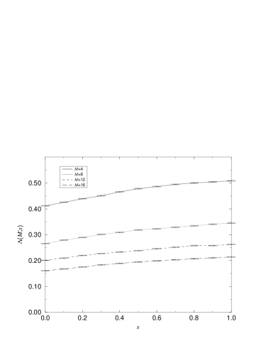
FIG. 9.: Renormalized localization length for strong disorder, $r=0.8$, $t=0.4$ which corresponds to $l_{\text{e}}\simeq 0.35$, depending on the spin scattering strength $s$ and the the system width $M$.

Contrary to this, the next example exhibits a LD transition at $s\simeq 0.3$, which can be seen in Fig. 10. With $r=0.55$ and $t=0.6$ corresponding to $l_{\text{e}}\simeq 1.1$ the effect of weak anti-localization causes the existence of extended states, if $s$ is strong enough. The intersection of the curves clearly indicates the LD transition. However, their slope is rather small compared to the error bars preventing an accurate scaling analysis close to the critical point.

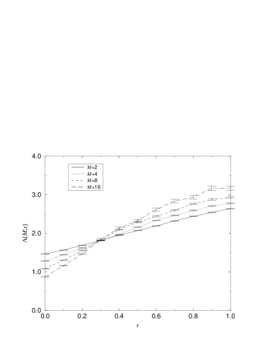
FIG. 10.: Renormalized localization length for $r=0.55$, $t=0.6$ which corresponds to $l_{\text{e}}\simeq 1.1$, depending on the spin scattering strength $s$ and the the system width $M$.

The third example shown in Fig. 11 belongs to the values $t=0.8$ and $s=0.4$, where $r$ varies from $r=0.48$ to $r=0.56$. It exhibits another kind of problem. Although curves for different system widths $M$ intersect, the points of intersection systematically depend on the width. The larger $M$ is the closer are the points of intersection for curves of neighboring values of $M$. It is obvious that there exists a limiting point, which would be the true critical point. The observed deviations are the consequence of finite-size effects, which vanish in the thermodynamic limit. By investigating $\Lambda$ at a lot of different points in parameter space we have seen that the deviations due to finite-size effects are larger for more delocalized systems. Actually, there is only a small area in parameter space that is suitable for a quantitative analysis of the LD transition.

FIG. 11.: Renormalized localization length in the vicinity of the localization-delocalization transition, $t=0.8$, $s=0.6$ which corresponds to $l_{\text{e}}\simeq 2$, depending on the reflection coefficient $r$ and the the system width $M$. The arrows mark the section of curves corresponding to neighbored values of $M$.

B Phase Diagram

We determined a phase diagram for the LD transition by using the scaling behavior of the RLL. More precisely, we calculated $\Lambda(M_{1}=4)$ and $\Lambda(M_{2}=8)$ for a lot of pairs $(r,t)$ with $s$ = 0.01, 0.02, 0.05, 0.1, 0.4 and 1. In order to get the critical line in the $(r,t)$-subspace with fixed $s$ we decided the point $(r,t,s)$ to be in the localized and delocalized regime, if

$$\Lambda(M_{1})-\Delta\Lambda(M_{1})\;>\;\Lambda(M_{2})+\Delta\Lambda(M_{2})$$ (78)

and

$$\Lambda(M_{2})-\Delta\Lambda(M_{2})\;>\;\Lambda(M_{1})+\Delta\Lambda(M_{1}),$$ (79)

respectively. In the case that both conditions failed, we considered the point in the parameter space to be critical. By that procedure we got a critical region, i.e. the separating line had some finite width. Fig. 12 shows the resulting phase diagrams for some intersections of the parameter space at the above declared fixed values of $s$. The white area marks the localized the grey one the delocalized phase. The drawn critical line is the optical interpolated center line of the critical region.

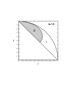
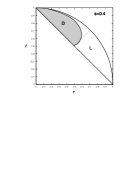
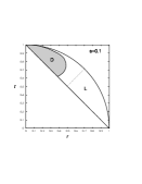
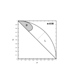
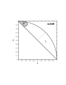
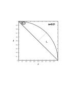
FIG. 12.: Phase diagrams for the localization-delocalization transition for cross-sections at $s=$ 1, 0.4, 0.1, 0.05, 0.02, 0.01. The grey area shows the delocalized, the white the localized regime. The dotted line corresponds to $r=t$.

The region of the metallic phase shrinks with decreasing spin scattering strength. This is due to the fact that the weak anti-localization then becomes less effective in preventing Anderson localization. At $s=0$ the system changes universality class from symplectic to orthogonal symmetry, a fact that could be verified by comparing the values of the localization lengths with those in Ref. [18]. On the other hand even a very small value of $s$ gives rise to a certain delocalized phase, if $r$ is small and $t$ is large enough. Of course, the larger $l_{e}$, i.e. the larger $t$ and smaller $r$, the more easily extended states occur. But even in the presence of full spin scattering only about the half of the area of the parameter space belongs to the metallic phase. This is due to the fact that parameter values $(r,t)$ belonging to the localized phase correspond to too strong disorder resulting in too strong localization to be broken by weak anti-localization.

It should be noticed, that for $t\gtrsim 0.6$ the shape of the phase boundary is influenced by finite-size effects. So the phase diagram can only serve as a qualitative picture of the LD transition. In order to improve on the phase diagram, one has to consider much larger systems, which is very computer time consuming taking such a large number of data points into account. Nevertheless, the lower part of the boundary, i.e. the region close to the line $r=t$ (dotted line in the figure), is suitable for quantitative investigations, as will be shown in the following.

C Scaling Function

We determined the scaling function by the fitting procedure described in Sec. IV A for $t=0.6$, $s=0.4$ and $r\in[0.52,0.62]$. In this small region of the phase space the corresponding curves $\Lambda(M;r)$ (see Fig. 13) are very well suitable for a quantitative analysis, because of their strong $r$ dependence and the absence of noticeable finite-size effects ($l_{\text{e}}\simeq 1$).

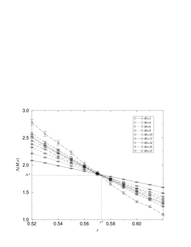
FIG. 13.: Renormalized localization length for $t=0.6$, $s=0.4$ which corresponds to $l_{\text{e}}\simeq 1$, depending on the reflection coefficient $r$ and the the system width $M$.

Fig. 14 shows the scaling function with the upper branch belonging to the metallic and the lower branch belonging to the localized regime. The curves represent the fitted Chebyshev polynomials. The data points are the raw data shifted by the fitted values of $\xi_{\text{c}}(r)$. We omitted the data with $M=2$ in the localized and $M=2$ and $M=4$ in the delocalized regime, because these values showed systematic deviations due to finite-size effects. Also data that are too close to the critical point were omitted. For the remaining data the confidence test of the fit gives $\Delta_{\Theta}=-0.30$ and $\Delta_{\Theta}=0.27$ for the localized and delocalized branch, respectively. So the assumption of one-parameter scaling is very well confirmed.

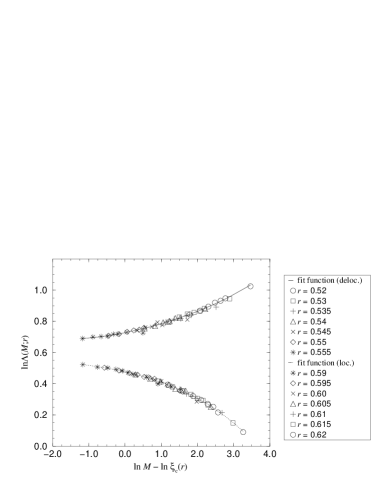
FIG. 14.: Scaling function for the localization-delocalization transition. The upper branch corresponds to the delocalized and the lower to the localized phase.

Fixing the fit parameters $\ln\xi_{\text{c}}$ by setting $\ln\xi_{\text{c}}(r=0.52)=0$ for the delocalized and $\ln\xi_{\text{c}}(r=0.62)=0$ for the localized branch (circles in Fig. 14) the procedure has converged with an accuracy of 0.1% after about 50 iterations. The starting values have a radius of convergence of about 5. So a rough estimate is sufficient for convergence.

The Chebyshev polynomials used are of fourth order. With a lower order it is impossible to fit the curves (as indicated by the figure of merit $\Delta_{\Theta}$), whereas with an order higher than 6 the fitted curves start to follow the fluctuations of the data points, which results in a non-physical behavior of the scaling function. With an order between four and six there is no significant difference in the results.

D Critical Exponent $\textstyle\nu$ and Critical RLL $\mathchoice{{\hbox{\boldmath$\displaystyle\Lambda$}}}{{\hbox{\boldmath$\textstyle\Lambda$}}}{{\hbox{\boldmath$\scriptstyle\Lambda$}}}{{\hbox{\boldmath$\scriptscriptstyle\Lambda$}}}^{\ast}$

In order to determine the critical exponent $\nu$ of the correlation length we used the fit procedure presented in Sec. IV C. With a starting value $r^{\ast}\in[0.53,0.59]$ the procedure converges. After about 10 iterations the corrections are smaller than 1%. The results of the fit are

$$\nu=2.51\pm 0.18\quad\text{and}\quad r^{\ast}=0.571\pm 0.002\;.$$ (80)

The prefactors take the values

$$\ln\xi_{\text{c}}^{\text{0,loc}}=-7.55\pm 0.42$$ (82)

and

$$\quad\ln\xi_{\text{c}}^{\text{0,deloc}}=-7.50-\pm 0.43.$$ (83)

The confidence test of the fit gives $\Delta_{\theta}=-0.47$, showing its high quality. It is very important to stress, that the given errors (Eq. (73)) are not independent. They have to be interpreted considering the correlation matrix

$${\sf C}_{\theta}=\left(\begin{array}[]{cccc}0.0310&-0.0737&-0.0739&-0.0004\\ -0.0737&0.1782&0.1766&0.0009\\ -0.0739&0.1766&0.1853&0.0009\\ -0.0004&0.0009&0.0009&5.5\cdot 10^{-6}\end{array}\right),$$ (84)

which shows that the different values are highly correlated.

Several reference values for $\nu$ have been published in the last years [27, 28, 29, 30]. The most recent calculations yield $\nu=2.75\pm 0.1$ [31], $\nu=2.5\pm 0.3$ [32] and $\nu=2.32\pm 0.14$ [33]. Within the errors our value agrees with these. We note that $\nu$ is very sensitive to slight variations of $r^{\ast}$. This is seen by fitting $\nu$ for fixed values of $r^{\ast}$. As is shown in Fig. 15 $\nu$ changes by 30% if $r^{\ast}$ changes by about 3%. The difficulties in obtaining a credible value for $\nu$ were the reasons to employ the iterative fit procedure of Sec. IV C.

FIG. 15.: Dependence of $\nu$ on the assumed value of $r^{\ast}$. The best estimate is found for $r^{\ast}=0.571$

In order to determine the critical RLL we used Eqs. (75) and (76). The result is

$$\Lambda^{\ast}=1.83\pm 0.03.$$ (85)

Finally, Eq. (45) yields the value for the scaling exponent of the typical LDOS

$$\alpha_{0}=2.174\pm 0.003.$$ (86)

This value agrees well with the result of Schweitzer [34], $\alpha_{0}=2.19\pm 0.03$ obtained for a Hamiltonian model.

VI Summary

In this work we found the S2NC-network model to be a new model to describe mesoscopic disordered electron systems with symplectic symmetry. We constructed the topology of the model and the scattering matrices representing the potential and spin scatterers. Three independent parameters were needed to characterize the scatterers. The reflection coefficient $r$ and the transmission coefficient $t$ represent the strength of the spatial disorder by defining the mean free path of the network model (in the absence of SOI). The coefficient $s$ represents the strength of the spin-orbit scattering and defines a corresponding spin scattering length. We have shown that our model exhibits a localization-delocalization transition. In order to investigate this transition we calculated renormalized localization lengths $\Lambda(r,t,s)$ by the transfer matrix method and obtained the scaling function by an iterative fit procedure. The quality of the fit was checked by a $\chi^{2}$-test, which confirmed the assumption of one-parameter scaling. We constructed a phase diagram for the system showing a metallic phase for any $s>0$, if $r$ is small and $t$ is large enough. The critical exponent of the correlation length was obtained to be $\nu=2.51\pm 0.18$. This value agrees with previously published results within the errors. We pointed out, that in determining the errors it is essential to take the correlations into account. The critical renormalized localization length was found to be $\Lambda^{\ast}=1.83\pm 0.03$. By a conformal mapping argument this corresponds to a value $\alpha_{0}=2.174\pm 0.003$ for the scaling exponent of the typical local density of states.

- [1] S. Kravchenko et al., Phys. Rev. B 50, 8039 (1994).
- [2] S. Kravchenko et al., Phys. Rev. B 51, 7038 (1995).
- [3] S. Kravchenko, D. Simonian, M. Sarachik, and W. M. J. Furneaux, Phys. Rev. Lett. 77, 4938 (1996).
- [4] V. Pudalov, G. Brunthaler, A. Prinz, and G. Bauer, JETP Lett 65, 1997 (1997).
- [5] D. Simonian, S. Kravchenko, and M. Sarachik, cond-mat/9704071.
- [6] D. Popović, A. Fowler, and S. Washburn, Phys. Rev. Lett. 79, 1543 (1997).
- [7] M. Simmons et al., cond-mat/9709240.
- [8] E. Abrahams, P. Anderson, D. Licciardello, and T. Ramakrishnan, Phys. Rev. Lett. 42, 673 (1979).
- [9] V. Dobrosavljević, E. Abrahams, E. Miranda, and S. Chakravarty, Phys. Rev. Lett. 79, 455 (1997).
- [10] S. Chakravarty, L. Yin, and E. Abrahams, cond-mat/9712217 .
- [11] V. Pudalov, JETP Lett. 66, 175 (1997).
- [12] C. Castellani, C. DiCastro, and P. Lee, cond-mat/9801006 .
- [13] Y. Lyanda-Geller, cond-mat/9801095 .
- [14] G. Bergmann, Solid State Comm. 42, 815 (1982).
- [15] S. Hikami, A. Larkin, and Y. Nagaoka, Prog. Theor. Phys. 63, 707 (1980).
- [16] S. Maekawa and H. Fukuyama, J. Phys. Soc. Japan 50, 2516 (1981).
- [17] P. Freche, M. Janssen, and R. Merkt, cond-mat/9710297; to be published in: Proccedings of the Ninth International Conference on Recent Progress in Many Body Theories, Sydney, Australia, 1997 .
- [18] P. Freche, Ph.D. thesis, Köln, 1997.
- [19] B. Huckestein, Physica A 167, 175 (1990).
- [20] M. Janßen, Int. Journal of Mod. Phys. B 8, 943 (1994).
- [21] F. Dyson, J. Math. Phys. 3, 140 (1962).
- [22] J. Chalker and P. Coddington, J. Phys. C 21, 2665 (1988).
- [23] A. Crisanti, G. Paladin, and A. Vulpiani, in Products of Random Matrices in Statistical Physics, edited by P. Fulde (Springer-Verlag, Berlin, 1992), Vol. 104, 26.
- [24] J. Pichard and G. Sarma, J. Phys. C 14, L127 (1981).
- [25] G. Bergmann, Phys. Rep. 107, 1 (1984).
- [26] B. Martin, Statistics for Physicists (Academic Press, London, 1971).
- [27] F. Wegner, Nucl. Phys. B 316, 663 (1989).
- [28] M. Zirnbauer, 4. DFG-Rundgespräch über den Quanten-Hall-Effekt, Schleching, 1989.
- [29] T. Ando, Phys. Rev. B 40, 5325 (1989).
- [30] A. MacKinnon, in Localization and Confinement of Electrons in Semiconductors, edited by F. Kuchar (Springer Series in Solid State Sciences, Berlin, 1990).
- [31] U. Fastenrath et al., Physica A 172, 302 (1991).
- [32] S. Evangelou, Phys. Rev. Lett. 75, 2550 (1995).
- [33] L. Schweitzer and I. Zharakeshev, J. Phys. Condens. Matter 9, L441 (1997).
- [34] L. Schweitzer, J. Phys. Condens. Matter 7, L281 (1995).