Berry-Robnik level statistics in a smooth billiard system
Tomaž Prosen

Department of Physics, Faculty of Mathematics and Physics,

University of Ljubljana, Jadranska 19, SLO-1111 Ljubljana, Slovenia

Abstract. Berry-Robnik level spacing distribution is demonstrated clearly in a generic quantized plane billiard for the first time. However, this ultimate semi-classical distribution is found to be valid only for extremely small semi-classical parameter (effective Planck’s constant) where the assumption of statistical independence of regular and irregular levels is achieved. For sufficiently larger semiclassical parameter we find (fractional power-law) level repulsion with phenomenological Brody distribution providing an adequate global fit.

PACS numbers: 05.45.+b, 03.65.Ge, 03.65.Sq

Submitted to Journal of Physics A: Math. Gen.

Energy level statistics of mixed quantum systems whose classical dynamics is partly regular and partly chaotic have been intensively studied over the past decade (see [1] and references therein), and this subject is still much less theoretically understood than the level statistics of the two extreme cases, namely completely chaotic (hyperbolic) systems [2, 3], and integrable systems [4]. However, it is believed that mixed systems, for example hydrogen atom in strong magnetic field [5], are generic in nature, at least among dynamical systems with few degrees of freedom. Although Berry and Robnik have developed a semiclassical theory of level spacing statistics for mixed systems back in 1984 [6], there has been a lot of confusion in the literature advocating various phenomenological models due to incompatibility of experimental or numerical data with the Berry-Robnik (BR) statistics (see a recent comment [7]). BR distribution is built on a simple and clean assumption of a statistically independent superposition of partial subspectra consisting of regular or chaotic levels (following an old Percivals’ idea [8] of classifying the quantum eigenstates of mixed systems as regular or chaotic). The sequence of regular levels, associated to eigenstates whose phase space distribution functions (e.g. Wigner or Husimi) localize on regions of regular motion, is assumed to have Poissonian statistics, whereas the sequences of chaotic levels, associated with eigenstates whose phase space distribution functions extend over chaotic components of classical phase space, are assumed to have GOE (or GUE if antiunitary symmetry is absent) statistics of ensembles of Gaussian random matrices. Further, it is crucial to note that the gap distribution $E(S)$, the probability that unfolded energy interval of length $S$ contains no levels, factorizes upon independent superposition of level sequences, so the 2-component BR distribution for a system with a single classically chaotic component of relative measure $\rho_{2}$ and regular components of complementary measure $\rho_{1}=1-\rho_{2}$ reads

$$E_{\rm BR}(S)=E_{\rm Poisson}(\rho_{1}S)E_{\rm GOE}(\rho_{2}S).$$ (1)

Note that $E_{\rm Poisson}(S)=\exp(-S)$ while for $E_{\rm GOE}(S)$ no closed-form expression exists (for the exact infinitely-dimensional GOE), and we have to rely on various expansions (we recommend Padé approximation published in [9]). The more common nearest neighbour level spacing distribution $P(S)$ is directly related to the gap distribution, simply as $P_{\rm BR}(S)=d^{2}E_{\rm BR}(S)/dS^{2}$.

However, for the validity of semiclassical BR formula, two conditions have to be satisfied. (i) The regular and irregular levels should not be correlated, i.e. the corresponding (Wigner or Husimi) phase-space distributions should not overlap. This is true if the quantum resolution scale in phase space, $\hbar^{1/2}$ (where $\hbar$ is the effective Planck’s constant), is small enough to resolve the essential features of the structure of classical phase space: $\hbar^{1/2}<$ (sizes of the main regular islands, widths of chaotic strips penetrating through regular islands, etc). (ii) The quantum relaxation time, i.e. the Heisenberg (break) time $t_{\rm break}=2\pi\hbar/\Delta E$ (where $\Delta E$ is the mean level spacing) should be larger than the classical ergodic time $t_{\rm erg}$ on the chaotic component, $t_{\rm break}>t_{\rm erg}$. When this is not true, one expects dynamical localization of eigenstates inside the chaotic component [1, 10, 11, 12].

Note that the BR statistics are incompatible with level repulsion, namely $P_{BR}(0)=1-\rho_{2}^{2}\neq 0$. If either (i) or (ii) is violated, one recovers level repulsion $P(S\rightarrow 0)\rightarrow 0$. Indeed, numerous numerical studies ([1, 7, 13] and references therein) give phenomenological support to the fractional power-law level repulsion which is usually very well globally captured by the phenomenological Brody distribution [14]

$$P_{\rm B}(S)=(\beta+1)bS^{\beta}\exp(-bS^{\beta+1}),\quad b=[\Gamma(1+(\beta+1)^{-1})]^{\beta+1}$$ (2)

In fact, even for a generic 2-dim toy system with a simple phase space structure (where (i) and (ii) have the largest chances to apply) having a small number of islands and well connected chaotic component, one may verify that (i) and (ii) are typically fulfilled only for sequential quantum numbers substantially larger than $\sim 10^{6}-10^{7}$ [10].

So it is not surprising that the ‘ultimate semiclassical’ BR statistics have so far been clearly demonstrated only in two toy systems: (1) in a rather abstract compactified standard map [15], and (2) in a 2-dim semi-separable oscillator [13, 10], which is dynamically a generic system but geometrically somewhat special. Here we give the first clear numerical demonstration of BR statistics in a generic billiard system with a smooth boundary. We consider classical and quantum motion of a free particle moving inside a bounded planar region which has a shape of a smoothly deformed circle. Billiard domain is described by the following function $r(\phi)$, giving the radial distance from the origin to the boundary as a function of the polar angle $\phi$,

$$r(\phi)=1+a\cos(4\phi).$$ (3)

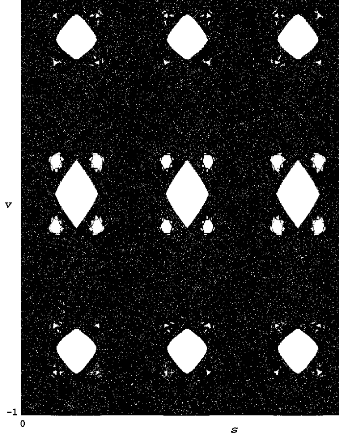
Figure 1: Classical phase space for $a=0.04$ in Poincaré-Birkhoff coordinates: arc-length $s$ and tangential (normalized) velocity $v$. We show a chaotic orbit with $2000000$ collisions with the boundary.

For the purpose of this letter we choose the following value of deformation parameter, $a=0.04$, for which the classical phase space (plotted in a Poincaré-Birkhoff coordinates on a boundary-section in figure 1) has regular regions with the total relative Liouville measure (not the area on SOS [16]) $\rho_{1}^{\rm cl}=0.115\pm 0.005$. Note that numerical computation of measures of regular and chaotic components of phase space in mixed (KAM) systems converges very slowly with increasing discretization of the phase space [17], hence it is difficult to further reduce the error estimate $\delta\rho_{1}^{\rm cl}\approx 0.005$.

High-lying quantum eigenenergies, eigenvalues of the Schrödinger equation $(\nabla^{2}+k^{2})\Psi_{k}(\vec{r})=0$ with Dirichlet b.c. on the boundary $r=r(\phi)$, have been computed by means of extremely efficient scaling technique proposed by Vergini and Saraceno [18]: Eigenstates $\Psi_{k}$ are expanded in a basis of circular scaling functions (see also [12], as opposed to plane waves used in original approach [18])

$$\Psi_{k}(\vec{r})=\sum_{l=1}^{M}a_{l}J_{4l}(kr)\sin(4l\phi).$$ (4)

Note that the billiard has been desymmetrized and here we consider only fully antisymmetric states with respect to 8-fold symmetry group of the billiard. The coefficients $a_{l}$ are determined by minimizing a special positive quadratic form defined along the boundary of the billiard [18]. The dimension of the problem $M=[(1+a)k/4]+M_{\rm evanescent}$ is nearly optimal where few ten, typically $M_{\rm evanescent}\sim 40$, evanescent modes have been added in order to ensure convergence and accuracy of the computed energy levels. We should note that the scaling method of quantization of billiards is by far superior to other relevant methods, e.g. boundary integral method [19] or Heller’s plane wave decomposition [20], since it yields a constant fraction ($5\%-10\%$) of $M\propto k$ of accurate levels, with no risk of missing any, by solving a single generalized eigenvalue problem of dimension $M$.

In figure 2 we show cumulative nearest neighbour level spacing distribution $W(S)=\int_{0}^{S}dsP(s)=(d/dS)E(S)-(d/dS)E(0)$ for the unfolded [9] spectral stretches $\{e_{n}=k_{n}^{2}/32+(1/8+1/\pi)k_{n};k_{\rm min}\leq k_{n}\leq k_{\rm max}\}$ (for small $a$) containing about $6000$ consecutive levels each. In fact, we have computed several spectral stretches, the first in the near semiclassical regime $399.7\leq k\leq 600.1$ (containing 6220 levels), and the last in the far semiclassical regime $15999.707\leq k\leq 16004.865$ (containing 5168 levels) where the sequential quantum number is $N\approx k^{2}/32+(1/8+1/\pi)k\approx 0.8\cdot 10^{7}$. Only for the last spectral stretch in the far semiclassical regime ($k\approx 16000$) we found statistically significant agreement with BR distribution (figures 2,3) where the quantal (best-fitting) parameter $\rho_{1}^{\rm q}$ agrees very well with its classical value, namely $\rho_{1}^{\rm q}=0.119$. However, for smaller sequential quantum numbers, when we approach the near-semiclassical regime, we find substantial deviation from BR statistics and recover fractional-power law level repulsion [21, 1], namely for the lowest spectral stretch (figures 2,3) at $k\approx 500$ we find almost statistically significant agreement with Brody distribution (2) with exponent $\beta=0.46$. Of course, the fit to BR distribution in the near semiclassical regime $k\approx 500$ and the fit to Brody distribution in the far semiclassical regime $k\approx 16000$ turned out to be highly statistically non-significant.

In figure 3 we show deviations of numerical spacing distributions from the semiclassical BR distribution (for parameter $\rho^{\rm q}_{1}=0.119\approx\rho^{\rm cl}_{1}$) in fine detail, using a smooth U-transformation [21] of the cumulative level spacing distribution $U(W(S))-U(W_{\rm BR}(S))$, where $U(W)=(2/\pi)\arccos\sqrt{1-W}$, against $W(S)$. This statistical representation has a uniform expected statistical error $\delta U(W)=1/(\pi\sqrt{\Delta N})$ (where $\Delta N$ is the number of levels in a spectral stretch) and a constant density of numerical points along the abscissa. One can see very clearly that in both cases, far and near semiclassical, the numerical distributions are fluctuating around theoretical BR and Brody distributions, respectively, within expected statistical error.

Finally we wish to characterize long-range spectral correlations as well, so we consider the number variance $\Sigma^{2}(L)=\left\langle N^{2}\right\rangle_{L}-\left\langle N\right\rangle^{2}_{L}$, i.e. the variance of the number of unfolded levels $e_{n}$ in an interval of length $L$. Since this is a linear statistic it should be additive upon statistically independent superposition of spectral subsequences [22]. According to assumptions (i) and (ii) one immediately arrives to the ultimate semiclassical formula for the number variance [22]

$$\Sigma^{2}(L)=\Sigma^{2}_{\rm Poisson}(\rho_{1}L)+\Sigma^{2}_{\rm GOE}(\rho_{2}L)$$ (5)

where $\Sigma^{2}_{\rm Poisson}(L)=L$ is the number variance of Poissonian level sequence, and $\Sigma^{2}_{\rm GOE}(L)\approx(2/\pi^{2})\ln(2\pi L)$ is the number variance of the spectrum of infinitely dimensional GOE random matrix which is supposed to model chaotic levels. In figure 4 we show $\Sigma^{2}(L)$ for four spectral stretches, namely for $k\approx 500$, $k\approx 2000$, $k\approx 8000$, and $k\approx 16000$, and only the last in the far semiclassical regime agrees well with the formula (5) (for parameter $\rho_{1}=\rho_{1}^{\rm cl}=0.115$) up to $L=L^{*}\approx 50$.

In this letter we have clearly demonstrated the validity of BR level spacing distribution in a generic smooth plane billiard system with mixed classical phase space, namely the quartic billiard. However, for insufficiently small semi-classical parameter $\hbar\sim N^{-1/2}$, we demonstrated the existence of fractional-power law level repulsion which is (for sufficiently small energy ranges) globally very well captured by the phenomenological Brody distribution. Unfortunately, this is the regime which can only be observed in most experimental situations due to extremely high energy region of crossover to BR statistics.

We should note that this particular KAM billiard system ((3) for $a=0.04$) has quite simple phase space structure which is reflected in relatively low transition point ($N\approx 10^{7}$) to the ultimate semiclassical BR statistics. For example, in a well known quadratic or Robnik billiard, the phase space is much more complicated [23] (smaller regular islands, more partial phase space bariers, cantori), and as a consequence, the transition to BR regime is shifted to much higher energies [24].

Figure captions

Figure 2: Cumulative nearest level spacing distribution $W(S)$ for a stretch of 5168 consecutive levels in the far semiclassical regime ($k\approx 16000$) (thick curve) and a stretch of 6220 consecutive levels in the near semiclassical regime ($k\approx 500$) (thin curve). The first numerical curve is almost overlapping with theoretical best fitting BR distribution for $\rho_{1}^{\rm q}=0.119$ (dashed curve), while the second numerical curve agrees very well with the best fitting Brody distribution with exponent $\beta=0.46$ (dot-dashed curve). For comparison we give Poisson and GOE integrated level spacing distributions (dotted curves). In the inset we plot the same data in the T-function representation [21], $T(S)=\ln(-\ln(1-W(S)))$ against $\ln S$, which transforms the Brody distributions (an hence also Poissonian and Wigner) to straight lines, and enhances the region of small spacings.

Figure 3: Fine detail deviations from Berry-Robnik distribution (for $\rho_{1}=0.119$) in a uniform U-function transformation [21]: we plot $U(W(S))-U(W_{\rm BR}(S))$ against $W(S)$. In the far semiclassical regime $k\approx 16000$ (5168 consecutive levels), the difference of U-functions (thick curve) lies within a band of expected statistical error $\delta U$ (dashed lines), while in the near semiclassical regime $k\approx 500$ (6220 consecutive levels), the difference of U-functions (thin curve) agrees very well with the difference of U-functions for the best fitting Brody distribution with exponent $\beta=0.46$ (dash-dotted curve).

Figure 4: Number variance $\Sigma^{2}(L)$ for the four spectral stretches: for $k\approx 16000$ (thickest curve, 5168 levels), $k\approx 8000$ (next thickest curve, 17300 levels), $k\approx 2000$ (second thinnest curve, 5100 levels), and $k\approx 500$ (thinnest curve, 6220 levels). Dashed curve is the semiclassical formula (5) which indeed reproduces the far semiclassical numerical data (thickest full curve) quite well, for $L\leq L^{*}\approx 50$. For comparison we give the Poissonian and GOE curves (dotted).

References

- [1] Prosen T and Robnik M 1994 J. Phys. A: Math. Gen. 27 8059
- [2] Andreev A V, Agam O, Simons B D, and Altshuler B L 1996 Phys.Rev.Lett. 76 3947
- [3] Bohigas O, in Proceedings of the 1989 Les Houches Smmer School on “Chaos and Quantum Physics”, ed. by M.J.Giannoni, A.Voros, J.Zinn-Justin (Elsevier Science Publisher B.V., North -Holland, Amsterdam 1991), p 89
- [4] Robnik M and Veble G “On spectral statistics of classically integrable systems”, preprint CAMTP/97-7, J. Phys. A: Math. Gen. in press, and references therein
- [5] Hasegawa H, Robnik M, and Wunner G 1989 Progress Theor. Phys. Suppl. 98 198; Friedrich H and Wintgen D 1989 Phys. Rep. 183 37
- [6] Berry M V and Robnik M 1984 J. Phys. A: Math. Gen. 17 2413
- [7] Robnik M and Prosen T 1997 J. Phys. A: Math. Gen. 30 8787
- [8] Percival I C 1973 J. Phys. B: At. Mol. Phys. 6 L229
- [9] Haake F “Quantum Signatures of Chaos” (Springer-Verlag, Berlin Heidelberg 1991)
- [10] Prosen T 1996 Physica D91 244
- [11] Borgonovi F, Casati G, and Li B 1996 Phys. Rev. Lett. 77 4744
- [12] Casati G and Prosen T 1998 “Quantum mechanics of chaotic billiards” preprint
- [13] Prosen T 1995 J. Phys. A: Math. Gen. 28 L349
- [14] Brody T A 1973 Lett. Nuovo Cimento 7 482
- [15] Prosen T and Robnik M 1994 J. Phys. A: Math. Gen. 27 L459
- [16] Meyer H D 1985 J. Chem. Phys. 84 3147
- [17] Robnik M, Dobnikar J, Rapisarda A, Prosen T, and Petkovšek M 1997 J. Phys. A: Math. Gen. 30 L803
- [18] Vergini E and Saraceno M 1995 Phys. Rev. E 52 2204
- [19] Berry M V and Wilkinson M 1984 Proc. R. Soc. Lond. A 392 15
- [20] Heller E J in Ref. [3], p 547
- [21] Prosen T and Robnik M 1993 J. Phys. A: Math. Gen. 26 2371
- [22] Seligman T H and Verbaarschot J J M 1985 J. Phys. A: Math. Gen. 18 2227
- [23] Robnik M 1983 J. Phys. A: Math. Gen. 16 3971
- [24] Robnik M, Liu J, and Veble G, work in progress