Finite-temperature properties of doped antiferromagnets

Abstract

We review recent results for the properties of doped antiferromagnets, obtained by the numerical analysis of the planar $t$-$J$ model using the novel finite-temperature Lanczos method for small correlated systems. First we shortly summarize our present understanding of anomalous normal-state properties of cuprates, and present the electronic phase diagram, phenomenological scenarios and models proposed in this connection. The numerical method is then described in more detail. Following sections are devoted to various static and dynamical properties of the $t$-$J$ model. Among thermodynamic properties the chemical potential, entropy and the specific heat are evaluated. Discussing electrical properties the emphasis is on the optical conductivity and the d.c. resistivity. Magnetic properties involve the static and dynamical spin structure factor, as measured via the susceptibility measurements, the NMR relaxation and the neutron scattering, as well as the orbital current contribution. Follows the analysis of electron spectral functions, being studied in photoemission experiments. Finally we discuss density fluctuations, the electronic Raman scattering and the thermoelectric power. Whenever feasible a comparison with experimental data is performed. A general conclusion is that the $t$-$J$ model captures well the main features of anomalous normal-state properties of cuprates, for a number of quantities the agreement is even a quantitative one. It is shown that several dynamical quantities exhibit at intermediate doping a novel universal behaviour consistent with a marginal Fermi-liquid concept, which seems to emerge from a large degeneracy of states and a frustration induced by doping the antiferromagnet.

to appear in ADVANCES IN PHYSICS

1 Introduction

The discovery of the high-temperature superconductivity (SC) in copper-oxide based compounds - cuprates (Bednorz and Müller 1986) revived the interest in materials containing transition elements. The main feature of these materials is the crucial role of electron-electron interactions. This can result in electronic properties, very unusual when compared to the behaviour of conventional metals. Although the unconventional SC is clearly the most puzzling phenomenon in cuprates, we focus in this review predominantly on the analysis of more or less anomalous properties of the normal state which deviate essentially from the standard understanding of electrons in metals and still present one of the major theoretical challenges in the solid state physics.

The cuprate superconductors have a very anisotropic structure, where the common building blocks are layers, in cuprates formed by combining one of the three possible structural elements containing Cu and O, as shown in Fig. 1.1b. The CuO layered structures are stacked in the crystal, separated by various intercalant layers in different cuprates. In spite of vast differences in the structure of unit cells, electronic properties of the whole family of cuprates are quite universal. This can be explained by the predominant role of generic CuO₂ planes, Fig. 1.1a, where conducting electrons reside. The electronic coupling between CuO₂ planes is very weak, resulting in a huge ratio of the in-plane resistivity to the perpendicular resistivity, in the anisotropy of the SC coherence length etc. Intermediate layers serve mainly as a charge reservoir for the planes. Consequently properties of cuprates are quite well classified according to the doping level of the reference CuO₂ electronic structure.

 

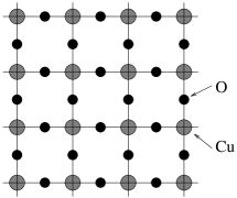
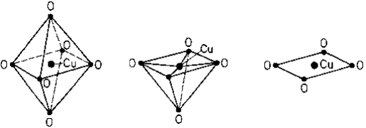
Figure 1.1: (a) Schematic structure of copper-oxide planes and (b) three possible building blocks of the planes, after Fulde (1991).

As now well established, the reference cuprate compounds, as La₂CuO₄ and YBa₂Cu₃O₆, are Mott (charge-transfer) insulators due to strong correlations which induce in a half-filled band a charge gap $\sim 2~{}$eV. The spin degrees of planar CuO₂ electrons can be well mapped on the properties of a planar antiferromagnetic (AFM) $S=1/2$ Heisenberg model. The AFM ground state of undoped materials, emerging from strong correlations, has been quite early recognized as a crucial starting point for theoretical considerations (Anderson 1987) of doped materials, being strange metals in the normal state and exhibiting high transition temperature $T_{c}$ to the SC state.

There are by now numerous indications that essential features of electronic properties of the doped AFM, as realized in cuprates, are well represented by prototype single-band models of correlated electrons, as the Hubbard model and the $t$-$J$ model (Rice 1995). In spite of their apparent simplicity both models are notoriously difficult to treat analytically, in particular in the most interesting regime of strong correlations. The lack of analytical tools for correlated electrons (for a general introduction see Fulde 1991) has increased the efforts towards numerical approaches (Dagotto 1994), which predominantly can be divided into two categories: the quantum Monte Carlo (QMC) methods and the exact diagonalization (ED) methods. The $t$-$J$ model, which incorporates the strong correlation requirement explicitly, is more adapted to the ED approach. So far most calculations were performed for the ground state (g.s.) at $T=0$, where the standard Lanczos technique (Lanczos 1950) offers an efficient ED analysis of small systems of reasonable sizes. Recently, present authors (Jaklič and Prelovšek 1994a) introduced a novel numerical method, combining the Lanczos method with a random sampling, which allows for an analogous treatment of statics and dynamics of many-body quantum models at $T>0$. The latter method, further referred to as the finite-temperature Lanczos method (FTLM), and results for the $t$-$J$ model obtained using this method, are the main subject of this review.

The final goal is to understand properties of doped AFM in general, and of high-$T_{c}$ cuprates in particular. In the absence of reliable analytical methods and results, numerical calculations can help to answer several crucial questions. Are strong correlations, as incorporated in prototype models, enough to account for anomalous normal-state properties of the strange metal ? Which are the relevant energy and temperature scales in doped AFM, as represented by the $t$-$J$ model, and in which properties do they show up ? Which is the unifying phenomenological description of the normal state ? Is the $t$-$J$ model sufficient, or which ingredients should be added to account qualitatively and quantitatively for observed properties ? Can we learn something macroscopically meaningful from the studies of small systems, and why ?

We note that at present the SC seems to be beyond the reach of numerical approaches including the FTLM, hence we do not investigate here in more detail the possible existence of SC and its origin in model systems.

2 Cuprates as doped antiferromagnets

2.1 Electronic phase diagram and properties of the normal state

Reference cuprate compounds are AFM insulators and are so far best understood. Properties of various other layered cuprates can be interpreted in terms of doping the reference material, where (mainly) holes are introduced into CuO₂ planes. One of the major conceptual achievements, which emerged from careful experimental investigations of high-quality materials in the last decade, has been the realization of quite universal electronic phase diagram (Hwang et al. 1994, Batlogg et al. 1994, Batlogg 1997), revealing characteristic temperature scales as they develop as the function of hole doping. It is at present quite common to classify materials with respect to doping as underdoped, optimally doped and overdoped, and the corresponding phase diagram is shown in Fig. 2.1.

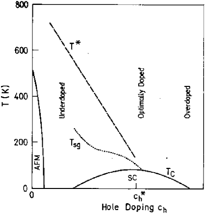
Figure 2.1: Schematic electronic phase diagram of cuprates, after Batlogg (1997).

2.1.1 Optimum doping regime

Experimentally optimum doping is chosen to correspond to materials with the highest $T_{c}$ within the given class of chemically and structurely related compounds. It has been realized soon after the discovery of high-$T_{c}$ SC that also normal state properties at $T>T_{c}$ of the optimally doped materials are very anomalous, but at the same time also most universal. The prominent feature is the resistivity law $\rho\propto T$ (Takagi et al. 1992), valid essentially in the whole measurable range $T>T_{c}$ and clearly contradicting the normal Landau-Fermi-liquid (LFL) behaviour $\rho\propto T^{2}$. Related is the observation that the dynamical conductivity $\sigma(\omega)$ does not fall off for larger $\omega$ according to the Drude form $\sigma\propto 1/\omega^{2}$, but rather as $\sigma\propto 1/\omega$ (Tanner and Timusk 1992).

The clearest evidence for an anomalous spin dynamics comes from the NMR and NQR relaxation (Slichter 1994), where the relaxation rate $1/T_{1}$ on planar ⁶³Cu in optimally doped La_2-xSr_xCuO₄ (LSCO) with $x_{opt}\sim 0.15$ is nearly $T$-independent (as well as nearly doping independent) in contrast to the usual Korringa law for metals $1/T_{1}\propto T$. The qualitative difference, i.e. a large enhancement of low-frequency spin fluctuations at low $T$, can be related to the persistence of short range AFM fluctuations, even at the optimum doping. The support for this comes also from neutron scattering experiments, where a substantial AFM correlation length $\xi$ has been measured in the same class of materials, with $\xi\sim 3.8\AA/\sqrt{x}$ (Birgeneau et al. 1988).

On the other hand, several properties at the optimum doping seem to be close to the normal LFL picture. The angle-resolved photoemission spectroscopy (ARPES) on cuprates (Shen and Dessau 1995), most reliable for BiSrCaCuO (BISCCO) compounds, shows electronic excitations consistent with a large Fermi surface (FS) and with the conserved FS volume (Luttinger theorem), although spectral shapes are quite distinct from a simple LFL picture. The specific heat (Loram et al. 1993) follows in the normal state roughly the LFL behaviour $C_{v}=\gamma T$ with $\gamma$ not very far from the free-fermion value, consistent with a nearly $T$-independent uniform susceptibility $\chi_{0}$, whereby the Wilson ratio is close to the free-fermion one (Loram et al. 1996). It is also the unifying characteristic of the optimum doping that properties do not reveal above $T_{c}$ any additional characteristic $T$ scale.

2.1.2 Overdoped and underdoped regime

In overdoped materials $T_{c}$ is decreasing and finally vanishing with increased doping. At the same time the electronic properties are getting closer to the usual metallic behaviour consistent with the LFL scenario. E.g., the resistivity behaviour moves towards the normal FLF form $\rho\propto T^{2}$ (Takagi et al. 1992), spectral shapes of electronic excitations, as revealed by ARPES, become sharper near the FS (Marshall et al. 1996) etc. These facts can be put together with a decreasing intensity of AFM fluctuations. It is thus plausible that we are dealing in the overdoped regime with the crossover to the normal LFL, however this crossover is not a trivial one and so far also not well understood either.

The most evident progress in the investigations of normal-state properties has been made in last few years for the underdoped cuprates. In contrast to the optimum doping, experiments reveal in this regime additional characteristic temperatures $T>T_{c}$ (Batlogg et al 1994), which show up as the crossovers where particular properties qualitatively change. As summarized in Fig. 2.1, there seems to be an indication for two distinct crossovers. The existence of both as well as their distinction is still widely debated, nevertheless we will refer to them as the AFM crossover scale $T^{*}$ and the pseudogap scale $T_{sg}$ for the lower one (Batlogg 1997).

The $T^{*}$ scale (Batlogg et al. 1994) shows up most clearly as the maximum of the spin susceptibility $\chi_{0}(T=T^{*})$ (Torrance et al. 1989). The in-plane resistivity $\rho(T)$ is linear $\rho\propto T$ for $T>T^{*}$ and decreases more steeply for $T<T^{*}$. Characteristic is also the anomalous $T$-dependence of the Hall constant $R_{H}(T)$ for $T<T^{*}$ (Ong 1990, Hwang et al. 1994). The latter is evidently hole-like in the classical sense $R_{H}(T\gtrsim T_{c})\propto 1/x$, which is also not properly understood theoretically. It seems plausible that the $T^{*}$ crossover is related to the onset of short-range AFM correlations for $T<T^{*}$, since in the undoped AFM $T^{*}$ corresponds just to a well understood maximum due to a gradual transition from a disordered paramagnet to the one with short-range AFM correlations.

The crossover $T_{sg}$ has been first identified in connection with the decrease of the NMR relaxation $1/T_{1}$ for $T<T_{sg}$ (Takigawa et al. 1991, Slichter 1994), indicating the reduction of low-energy spin excitations interpreted as the opening of the spin pseudogap in underdoped materials. Most striking evidence for an additional energy scale in underdoped cuprates is the observation of the leading-edge shift in ARPES measurements at $T>T_{c}$ (Marshall et al 1996), indicating features of the $d$-wave SC gap persisting within the normal phase. It should be pointed out, however, that the designation of crossover features is at present still controversial. In particular it is not evident whether we are dealing with two or more essentially different energy scales.

2.2 Phenomenology of the normal state

Properties of the normal LFL follow from the one-to-one correspondence of low-energy excitations of the interacting fermion system to that of a free-fermion gas. The prerequisite is that the volume of the FS is conserved (Luttinger 1960). Essential are the well defined quasiparticles (QP) with the vanishing damping at the FS, with $\Gamma\propto(E-E_{F})^{2}$. Consequences are the linear specific heat $C_{V}=\gamma T$, nearly $T$-independent static and dynamical spin susceptibilities, the Korringa law for NMR relaxation $1/T_{1}\propto T$, the resistivity $\rho(T)\propto T^{2}$ etc. Experimental facts on cuprates contradict the usual LFL picture. Several more or less elaborated scenarios have been proposed to capture main anomalous features.

Focusing on the importance of AFM spin fluctuations, the concept of a nearly AFM Fermi liquid (NAFL) has been elaborated (see e.g. Monthoux and Pines 1994). Here one assumes that at low-frequencies $\chi^{\prime\prime}(\vec{q},\omega)\propto\omega$ at all $\vec{q}$, as expected in a LFL, but with strongly enhanced fluctuations near the AFM wavevector $\vec{Q}=(\pi,\pi)$, corresponding to the critical slowing down in the proximity of a phase transition to the AFM-ordered state. The following form has been proposed, which can be derived also via the self-consistent paramagnon theory (Moriya et al. 1990),

$$\chi(\vec{q},\omega)=\frac{\chi_{\vec{Q}}}{1+\xi^{2}|\vec{q}-\vec{Q}|^{2}-i\omega/\omega_{SF}}\;.$$ (2.1)

In the proposal by Millis et al. (1990), originally devoted to the interpretation of the NMR and NQR relaxation, the main $T$-dependence is expected to arise from the AFM correlation length $\xi$, which is assumed to show a critical behaviour as $T$ is decreased, i.e. $\xi^{2}\propto T_{x}/(T+T_{x})$. In order to explain the anomalous NQR relaxation $1/T_{1}(T)\sim const$ (Imai et al. 1993), contradicting the Korringa law, strong $T$-dependence of $\xi$ is essential with $T_{x}\sim 100~{}K$, as well as low $\omega_{SF}$ and large $\chi_{\vec{Q}}$ for $T\sim T_{c}$ (Monthoux and Pines 1994). The form of spin fluctuations is the basis for further investigations of the charge dynamics, strongly coupled to spin degrees of freedom. The calculated response functions such as the conductivity appear also anomalous, e.g. the resistivity is close to a linear law $\rho\propto T$.

There are several proposals, analogous to the NAFL in the basic idea of the proximity to a critical point, enhancing fluctuations in the optimum doping regime. One proposal invokes the quantum critical scaling of the spin dynamics, established in the nonlinear sigma model (Chakravarty et al. 1989), induced by doping the AFM (Sokol and Pines 1993). Another scenario relates the quantum critical point to a charge-density-wave instability (Castellani et al. 1995).

An alternative interpretation of experimental facts has been provided by the concept of a marginal Fermi liquid (MFL) (Varma et al. 1989). The hypothesis is that there exist excitations, contributing both to the charge and spin response, which show in a broad range of wavevectors $\vec{q}$ anomalous susceptibilities of the form

$$\chi^{\prime\prime}(\vec{q},\omega)\sim\left\{{C~{}\omega/T~{}~{}~{}{\rm for}~{}~{}~{}|\omega|<T,\atop C~{}{\rm sgn}\,\omega~{}~{}~{}{\rm for}~{}~{}~{}|\omega|>T}\right.$$ (2.2)

Due to the scattering on bosonic excitations with the spectrum (2.2) the single-particle self-energy $\Sigma(\vec{k},\omega)$ is also anomalous. Assuming its $\vec{k}$-independence in a broad range, it has been postulated using phenomenological arguments (Littlewood and Varma 1991),

$$\Sigma(\omega)\sim\pi\lambda\left[2\omega\ln\frac{x}{\omega_{c}}-ix\right],\qquad x=\max(|\omega|,\pi T),$$ (2.3)

where $\omega_{c}$ is a high-frequency cutoff. Hence the QP lifetime $1/\tau\propto-\Sigma^{\prime\prime}(\omega)$ is anomalous, i.e. $1/\tau(\omega)\propto x$. It should be however mentioned that the Ansatz (2.3) is not unique and also modified forms have been invoked, e.g. in the analysis of the optical conductivity (El Azrak et al. 1994, Baraduc et al. 1995) better fit has been obtained with

$$-\Sigma^{\prime\prime}(\omega)\sim\pi\lambda(|\omega|+\pi T).$$ (2.4)

While the FS should remain well defined with the volume equal to that of free fermions, the corresponding QP weight $\tilde{Z}$ at the FS, given by

$$\tilde{Z}^{-1}=1-\partial\Sigma^{\prime}(\omega)/\partial\omega|_{\omega=0},$$ (2.5)

vanishes on the FS in analogy to the case of a one-dimensional Luttinger liquid (Haldane 1981). The MFL concept accounts for several remarkable properties at the optimum doping, as the anomalous resistivity $\rho(T)\propto T$, the optical conductivity $\sigma(\omega)\propto 1/\omega$, the NMR and the NQR relaxation rate $1/T_{1}(T)\sim const$. Note that the only low-energy scale within the MFL scenario, equations (2.2) - (2.4), is given by $T$. Although there are certain similarities to the NAFL and other critical-point scenarios, the essential difference of the MFL concept is a non-critical $\vec{q}$ dependence. Hence the critical behaviour within the MFL is rather a local one. The attempts to derive MFL behaviour from a microscopic model have not been successful so far.

2.3 Models of correlated electrons in cuprates

A similarity of electronic properties in a wide class of different cuprates serves as a strong indication that the appropriate microscopic model should be quite universal and must in first place describe the electrons restricted to CuO₂ orbitals within a single plane. There has been quite an extensive effort put into finding a proper model, and at present there seems to be a wide consensus on its main features. This should be contrasted to various other materials with interacting electrons, e.g. heavy fermions and 1D conductors, where microscopic models are much less known.

Since the physics of electrons in CuO₂ planes is governed by Cu $3d_{x^{2}-y^{2}}$ orbitals and O $2p_{x,y}$ orbitals (see the structure in Fig. 1.1), quite a complete model seems to be the three-band Hubbard model (Emery 1987), describing fermion carriers (holes) added to closed $3d^{10}$ and $2p^{6}$ shells. Parameters are the Cu–O hopping $t_{pd}$, the direct O–O hopping $t_{pp}$, the on-site energies $\varepsilon_{d}$, $\varepsilon_{p}$, and the corresponding Coulomb repulsions $U_{d}$, $U_{p}$ on Cu and O sites, respectively. Parameters correspond to the charge-transfer regime with $\Delta=\varepsilon_{p}-\varepsilon_{d}>t_{pd}$ and $U_{d}>\Delta$. The reference (insulator) material contains one fermion/cell, entering predominantly the $d$ orbitals. Due to $U_{d}\gg t_{pd}$, a large charge gap $\sim 2$eV opens at half filling, while spin degrees can be mapped on the isotropic $S=1/2$ Heisenberg model, first proposed in connection with cuprates by Anderson (1987). Holes added by doping enter the singlets, introduced by Zhang and Rice (1988), which can be in a fermion model treated as empty sites (holes). Such a reduction, confirmed also with other analytical approaches (Zaanen and Oleś 1988, Ramšak and Prelovšek 1989) and cluster methods (Hybertsen et al. 1990), leads to a single-band $t$-$J$ model (Rice 1995),

$$H=-t\sum_{\langle ij\rangle s}(\tilde{c}^{\dagger}_{js}\tilde{c}_{is}+{\rm H.c.})+J\sum_{\langle ij\rangle}(\vec{S}_{i}\cdot\vec{S}_{j}-{1\over 4}n_{i}n_{j}),$$ (2.6)

describing fermions in a tight-binding band with the hopping parameter $t\propto t_{pd}^{2}/\Delta$. Here $\vec{S}_{i}=(1/2)\sum_{ss^{\prime}}c^{\dagger}_{is}\vec{\sigma}_{ss^{\prime}}c_{is^{\prime}}$ are the local spin operators interacting with the exchange parameter $J\propto t^{4}_{pd}/U_{d}\Delta<t$. Due to the strong on-site repulsion states with doubly occupied sites are explicitly forbidden and we are dealing with projected fermion operators $\tilde{c}_{is}=c_{is}(1-n_{i,-s})$.

By explicitly projecting out states with doubly occupied sites, the $t$-$J$ model only allows for charge fluctuations in terms of a hole motion, while at half-filling it is equivalent to the $S=1/2$ Heisenberg model. The $t$-$J$ model is expected to capture the essential low-energy physics of doped AFM as well of cuprates in the whole regime of dopings. The challenging regime of the model is the one of strong correlations with $J<t$.

The $t$-$J$ model is the simplest model which describes the interplay of magnetism and itinerant metallic properties of cuprates. A more rigorous reduction of the three-band model (Zaanen and Oleś 1988, Ramšak and Prelovšek 1989) leads to additional terms, which could be as well represented within a reduced space without doubly occupied sites. Among possible generalizations most attention has been recently devoted to the addition of the next-nearest-neighbour (n.n.n.) hopping ($t^{\prime}$) terms, emerging from the $t_{pp}$ hopping in the three-band model,

$$H_{t^{\prime}}=-t^{\prime}\sum_{\langle\langle ij\rangle\rangle s}(\tilde{c}^{\dagger}_{js}\tilde{c}_{is}+{\rm H.c.}),$$ (2.7)

representing the hopping along the diagonal in Fig. 1.1a. Analogous is the $t^{\prime\prime}$ term for the n.n.n. hopping along each axis. It seems necessary to include such a term to account for the QP dispersion found in ARPES experiments on undoped material, such as Sr₂CuO₂Cl₂ (Wells et al. 1995). In spite of their apparent smallness, $t^{\prime}$ and $t^{\prime\prime}$ terms could lead to relevant corrections since they allow a free propagation of fermions even in an AFM (Néel) spin background.

The $t$-$J$ model, as relevant for cuprates, should be considered on a planar square lattice. Parameters are rather well known (Rice 1995). $J$ is measured in the undoped AFM via the inelastic neutron scattering and the magnon dispersion, leading to $J\sim 0.13$ eV. The hopping parameter $t$ is not accessible directly, but cluster calculations (Hybertsen el al. 1990) and other considerations (Rice 1995) allow only for a narrow range of $t$ values. In our calculations we shall furtheron use (if not declared differently) $t=0.4$ eV and $J/t=0.3$.A possible range for $t^{\prime}$ (Hybertsen et al. 1990) is more controversial, while in numerical studies (Tohyama and Maekawa 1994, Nazarenko et al. 1995) values $-0.35<t^{\prime}/t<-0.2$ are used.

Another prototype model for strongly correlated electrons is the traditional Hubbard model (Hubbard 1963),

$$H=-t\sum_{\langle ij\rangle s}(c^{\dagger}_{js}c_{is}+{\rm H.c.})+U\sum_{i}n_{i\uparrow}n_{i\downarrow}.$$ (2.8)

High-energy excitations of the Hubbard model could be different from those of the charge-transfer regime in the three-band model, still it is expected that the low-energy properties map well on those of the $t$-$J$ model provided that $U\gg t$. In the following we shall mainly consider $T>0$ properties of the $t$-$J$ model. It should be however noted that prior to the introduction of the FTLM method most calculations of $T>0$ properties have been performed for the Hubbard model by applying QMC methods (Dagotto 1994).

3 Finite-Temperature Lanczos Method

This chapter is devoted to the description of the FTLM which we developed (Jaklič and Prelovšek 1994a) for studying correlated systems at $T>0$ and which is used to obtain results described furtheron. The goal was to calculate $T>0$ properties in small model systems and to find a method, comparable in efficiency to g.s. calculations employing ED methods, used in the past decade extensively in the study of correlated systems (Dagotto 1994).

Here we should stress that the advantage of $T>0$ calculations is twofold. It is evident that we are interested in static and dynamical properties at nonzero $T$, in particular in their $T$-variation. On the other hand, the use of finite but small $T>0$ represents the proper approach to more reliable g.s. calculations in small systems. Namely, it is well known that g.s. ED results, in particular for dynamical quantities, are strongly influenced by finite size artifacts. At $T>0$ the latter effects can to large extent average out, leading to more macroscopic-like results. Still the understanding of remaining finite-size restrictions is important for the proper application of the method, as will be described in Sec. 3.7. In Sec. 3.8. we put our approach in perspective with other methods yielding $T>0$ results for models of correlated electrons. These includes mainly various QMC methods and the high-$T$ expansion (HTE) technique.

3.1 Lanczos algorithm and matrix elements

The scarcity of well-controlled analytical approaches to models of strongly correlated electrons has stimulated the development of computational methods. Conceptually the simplest is the ED method of small systems. In models of correlated electrons, however, one is dealing with the dimension of the basis (number of basis states) which grows exponentially with the size of the system. In the Hubbard model there are 4 basis states for each lattice site, therefore the number of basis states in the $N$-site system is $N_{st}\propto 4^{N}$. In the $t-J$ model $N_{st}$ still grows as $\propto 3^{N}$. In the ED of such systems one is therefore representing operators with matrices $N_{st}\times N_{st}$, which become large already for very modest values of $N$. The helpful circumstance is that for most interesting operators and lattice models only a small proportion of matrix elements is nonzero within the local basis. Then, the operators can be represented by sparse matrices with $N_{st}$ rows and at most $f(N)$ nonzero elements in each row. In this way memory requirements are relaxed and matrices up to $N_{st}\sim 10^{7}$ are considered in recent applications. Finding eigenvalues and eigenvectors of such large matrices is not possible with standard algorithms performing the full diagonalization. One must instead resort to the power algorithms (see Parlett 1980), among which the Lanczos algorithm (Lanczos 1950) is one of the most widely known.

The Lanczos algorithm starts with a normalized random vector $|\phi_{0}\rangle$ in the vector space in which the Hamiltonian operator $H$ is defined. $H$ is applied to $|\phi_{0}\rangle$ and the resulting vector is split in components parallel to $|\phi_{0}\rangle$, and $|\phi_{1}\rangle$ orthogonal to it, respectively,

$$H|\phi_{0}\rangle=a_{0}|\phi_{0}\rangle+b_{1}|\phi_{1}\rangle.$$ (3.1)

Since $H$ is Hermitian, $a_{0}=\langle\phi_{0}|H|\phi_{0}\rangle$ is real, while the phase of $|\phi_{1}\rangle$ can be chosen so that $b_{1}$ is also real. In the next step $H$ is applied to $|\phi_{1}\rangle$,

$$H|\phi_{1}\rangle=b_{1}^{\prime}|\phi_{0}\rangle+a_{1}|\phi_{1}\rangle+b_{2}|\phi_{2}\rangle,$$ (3.2)

where $|\phi_{2}\rangle$ is orthogonal to $|\phi_{0}\rangle$ and $|\phi_{1}\rangle$. It follows also $b_{1}^{\prime}=\langle\phi_{0}|H|\phi_{1}\rangle=b_{1}$. Proceeding with the iteration one gets in $i$ steps

$$H|\phi_{i}\rangle=b_{i}|\phi_{i-1}\rangle+a_{i}|\phi_{i}\rangle+b_{i+1}|\phi_{i+1}\rangle,\qquad 1\leq i\leq M.$$ (3.3)

By stopping the iteration at $i=M$ and putting the last coefficient $b_{M+1}=0$, the Hamiltonian can be represented in the basis of orthogonal Lanczos functions $|\phi_{i}\rangle$ as the tridiagonal matrix $H_{M}$ with diagonal elements $a_{i}$ with $i=0\ldots M$, and offdiagonal ones $b_{i}$ with $i=1\ldots M$. Such a matrix is easily diagonalized using standard numerical routines to obtain approximate eigenvalues $\epsilon_{j}$ and the corresponding orthonormal eigenvectors $|\psi_{j}\rangle$,

$$|\psi_{j}\rangle=\sum_{i=0}^{M}v_{ji}|\phi_{i}\rangle,\;\;\;j=0\ldots M.$$ (3.4)

It is important to realize that $|\psi_{j}\rangle$ are (in general) not exact eigenfunctions of $H$, but show a remainder

$$H|\psi_{j}\rangle-\epsilon_{j}|\psi_{j}\rangle=b_{M+1}v_{jM}|\phi_{M+1}\rangle.$$ (3.5)

On the other hand it is evident from the diagonalization of $H_{M}$ that matrix elements

$$\langle\psi_{i}|H|\psi_{j}\rangle=\epsilon_{j}\delta_{ij},\;\;\;i,j=0\ldots M$$ (3.6)

are exact, without restriction to the subspace $L_{M}$.

If in the equation (3.3) $b_{M+1}=0$, we have found a $(M+1)$-dimensional eigenspace where $H_{M}$ is already an exact representation of $H$. This inevitably happens when $M=N_{st}-1$, but for $M<N_{st}-1$ it can only occur if the starting vector is orthogonal to some invariant subspace of $H$. This should not be the case if the input vector $|\phi_{0}\rangle$ is random, without any hidden symmetries.

The number of operations needed to perform $M$ Lanczos iterations scales as $MN_{st}$. Numerically the Lanczos procedure is subject to roundoff errors, introduced by the finite-precision arithmetics. This problem usually only becomes severe at larger $M>100$ (more than needed to get accurate g.s. $|\psi_{0}\rangle$) and is seen in the loss of the orthogonality of vectors $|\phi_{i}\rangle$. It can be remedied by successive reorthogonalization (and normalization) of new states $|\phi^{\prime}_{i}\rangle$, plagued with errors, with respect to previous ones. However this procedure requires $\sim M^{2}N_{st}$ operations, and can become computationally more demanding than Lanczos iterations alone. This effect prevents one to use the Lanczos method e.g. to tridiagonalize large matrices.

The identity (3.6) already shows the usefulness of the Lanczos method for the calculation of particular matrix elements. As an aid in a further discussion of the Lanczos method we consider the calculation of a matrix element

$$W_{kl}=\langle n|H^{k}BH^{l}A|n\rangle,$$ (3.7)

where $|n\rangle$ is an arbitrary normalized vector, and $A,B$ are general operators. One can calculate this expression exactly by performing two Lanczos procedures with $M=\max(k,l)$ steps. The first one, starting with the vector $|\phi_{0}\rangle=|n\rangle$, produces the subspace $L_{M}=\{|\phi_{j}\rangle,\;j=0\ldots M\}$ along with approximate eigenvectors $|\psi_{j}\rangle$ and eigenvalues $\epsilon_{j}$. The second Lanczos procedure is started with the normalized vector

$$|\tilde{\phi}_{0}\rangle=A|\phi_{0}\rangle/\sqrt{\langle\phi_{0}|A^{\dagger}A|\phi_{0}\rangle},$$ (3.8)

and results in the subspace $\tilde{L}_{M}=\{|\tilde{\phi}_{j}\rangle,\;j=0\ldots M\}$ with approximate $|\tilde{\psi}_{j}\rangle$ and $\tilde{\epsilon}_{j}$. We can now define projectors

$$P_{m}=\sum_{i=0}^{m}|\phi_{i}\rangle\langle\phi_{i}|,\;\;\tilde{P}_{m}=\sum_{i=0}^{m}|\tilde{\phi}_{i}\rangle\langle\tilde{\phi}_{i}|,$$ (3.9)

which for $m=M$ can also be expressed as

$$P_{M}=\sum_{i=0}^{M}|\psi_{i}\rangle\langle\psi_{i}|,\;\;\tilde{P}_{M}=\sum_{i=0}^{M}|\tilde{\psi}_{i}\rangle\langle\tilde{\psi}_{i}|.$$ (3.10)

By taking into account definitions (3.9), (3.10) we show that

$$HP_{m}=P_{m+1}HP_{m}=P_{M}HP_{m},\qquad m<M.$$ (3.11)

Since in addition $|n\rangle=|\phi_{0}\rangle=P_{0}|\phi_{0}\rangle$ and $A|n\rangle\propto|\tilde{\phi}_{0}\rangle=P_{0}|\tilde{\phi}_{0}\rangle$, by successive use of the first equality in (3.11) we arrive at

$$W_{kl}=\langle\phi_{0}|P_{0}HP_{1}H\ldots HP_{k}B\tilde{P}_{l}H\ldots\tilde{P}_{1}H\tilde{P}_{0}A|\phi_{0}\rangle.$$ (3.12)

Using the second equality in the equation (3.11) and identities $P_{0}|\phi_{0}\rangle=P_{M}|\phi_{0}\rangle$, $\tilde{P}_{0}A|\phi_{0}\rangle=\tilde{P}_{M}A|\phi_{0}\rangle$ we can rewrite $W_{kl}$ as

$$W_{kl}=\langle\phi_{0}|P_{M}HP_{M}H\ldots HP_{M}B\tilde{P}_{M}H\ldots\tilde{P}_{M}H\tilde{P}_{M}A|\phi_{0}\rangle.$$ (3.13)

We note that the necessary condition for the equation (3.13) is $M\geq k,l$. We finally expand the projectors according to expressions (3.10) and take into account the orthonormality relation (3.6) for matrix elements, and get

$$W_{kl} = \sum_{i_{0}=0}^{M}\ldots\sum_{i_{k}=0}^{M}\sum_{j_{0}=0}^{M}\ldots\sum_{j_{l}=0}^{M}\langle\phi_{0}|\psi_{i_{0}}\rangle\langle\psi_{i_{0}}|H|\psi_{i_{1}}\rangle\ldots\langle\psi_{i_{k-1}}|H|\psi_{i_{k}}\rangle$$ (3.14)

$$\times\langle\psi_{i_{k}}|B|\tilde{\psi}_{j_{l}}\rangle\langle\tilde{\psi}_{j_{l}}|H|\tilde{\psi}_{j_{l-1}}\rangle\ldots\langle\tilde{\psi}_{j_{1}}|H|\tilde{\psi}_{j_{0}}\rangle\langle\tilde{\psi}_{j_{0}}|A|\phi_{0}\rangle=$$

$$= \sum_{i=0}^{M}\sum_{j=0}^{M}\langle\phi_{0}|\psi_{i}\rangle\langle\psi_{i}|B|\tilde{\psi}_{j}\rangle\langle\tilde{\psi}_{j}|A|\phi_{0}\rangle(\epsilon_{i})^{k}(\tilde{\epsilon}_{j})^{l}.$$

We have thus expressed the desired quantity in terms of the Lanczos (approximate) eigenvectors, and eigenvalues alone.

3.2 Dynamical response in the ground state

Within the Lanczos algorithm the extreme (smallest and largest) eigenvalues $\epsilon_{i}$, along with their corresponding $|\psi_{i}\rangle$, are rapidly converging to exact eigenvalues $E_{i}$ and eigenvectors $|\Psi_{i}\rangle$. It is quite characteristic that usually (for nondegenerate states) $M=30-60\ll N_{st}$ is sufficient to achieve the convergence to the machine precision of the g.s. energy $E_{0}$ and the wavefunction $|\Psi_{0}\rangle$, from which various static and dynamical correlation functions at $T=0$ can be evaluated.

After $|\Psi_{0}\rangle$ is obtained, the g.s. dynamic correlation functions can be calculated within the same framework (Haydock et al. 1972). Let us consider the autocorrelation function

$$C(t)=-i\langle\Psi_{0}|A^{\dagger}(t)A|\Psi_{0}\rangle=-i\langle\Psi_{0}|A^{\dagger}e^{i(E_{0}-H)t}A|\Psi_{0}\rangle$$ (3.15)

with the transform,

$$\tilde{C}(\omega)=\int_{0}^{\infty}dte^{i\omega^{+}t}C(t)=\langle\Psi_{0}|A^{\dagger}\frac{1}{\omega^{+}+E_{0}-H}A|\Psi_{0}\rangle.$$ (3.16)

where $\omega^{+}=\omega+i\epsilon,~{}\epsilon>0$. To calculate $\tilde{C}(\omega)$, one has to run the second Lanczos procedure starting with the normalized function $|\tilde{\phi}_{0}\rangle$, equation (3.8). The matrix for $H$ in the new basis $\tilde{L}_{M}$, with elements $\langle\tilde{\phi}_{i}|H|\tilde{\phi}_{j}\rangle=[\tilde{H}_{M}]_{ij}$, is again a tridiagonal one with $\tilde{a}_{i}$ and $\tilde{b}_{i}$ elements, respectively. Terminating the Lanczos procedure at given $M$, one can evaluate the $\tilde{C}(\omega)$ as a resolvent of the $\tilde{H}_{M}$ matrix which can be expressed in the continued-fraction form (Haydock et al. 1972),

$$\tilde{C}(\omega)=\frac{\langle\Psi_{0}|A^{\dagger}A|\Psi_{0}\rangle}{\omega^{+}+E_{0}-\tilde{a}_{0}-{\displaystyle\frac{\tilde{b}_{1}^{2}}{\omega^{+}+E_{0}-\tilde{a}_{1}-{\displaystyle\frac{\tilde{b}_{2}^{2}}{\omega^{+}+E_{0}-\tilde{a}_{2}-\ldots}}}}}\;,$$ (3.17)

terminating with $\tilde{b}_{M+1}=0$, although other termination functions have also been employed.

The spectral function $C(\omega)=-(1/\pi){\rm Im}\tilde{C}(\omega)$ is characterized by frequency moments,

$$\mu_{l}=\int_{-\infty}^{\infty}\omega^{l}C(\omega)d\omega=\langle\Psi_{0}|A^{\dagger}(H-E_{0})^{l}A|\Psi_{0}\rangle,$$ (3.18)

which are particular cases of the expression (3.7) for $B=A^{\dagger}$, $k=0$, and $|n\rangle=|\Psi_{0}\rangle$. Using the equation (3.14) we can express $\mu_{l}$ for $l\leq M$ in terms of Lanczos quantities alone

$$\mu_{l}=\sum_{j=0}^{M}\langle\Psi_{0}|A^{\dagger}|\tilde{\psi}_{j}\rangle\langle\tilde{\psi}_{j}|A|\Psi_{0}\rangle(\tilde{\epsilon}_{j}-E_{0})^{l}.$$ (3.19)

Hence moments are exact for given $|\Psi_{0}\rangle$ (as would be also for any other starting $|n\rangle$) provided $l\leq M$. The corresponding approximation for $C(t)$, equation (3.15), within the restricted set of eigenfunctions $|\tilde{\psi}_{j}\rangle,j=0\ldots M$, can be written at given $M$ (assuming $\tilde{b}_{M+1}=0$) as

$$C(t)=-i\sum_{j=0}^{M}\langle\Psi_{0}|A^{\dagger}|\tilde{\psi}_{j}\rangle\langle\tilde{\psi}_{j}|A|\Psi_{0}\rangle e^{-i(\tilde{\epsilon}_{j}-E_{0})t}.$$ (3.20)

Note that such $C(t)$ expanded as a series in $t$ (short-time expansion) has exact $M$ terms, since the coefficients are just moments $\mu_{l}$, equation (3.19).

As a practical matter we note that $|\langle\tilde{\psi}_{j}|A|\Psi_{0}\rangle|^{2}=\tilde{v}_{j0}^{2}$, hence no matrix elements need to be evaluated within this approach. In contrast to the continued fraction (3.17), the expression (3.20) allows also the treatment of more general correlation functions $\langle B(t)A\rangle$, with $B\neq A^{\dagger}$. In this case the matrix elements $\langle\Psi_{0}|B|\tilde{\psi}_{j}\rangle$ have to be evaluated explicitly. From the above one sees that the Lanczos method is very convenient to calculate the frequency moments as well as the dynamical $C(\omega)$. Certain ideas presented above will be used to construct the algorithm for $T>0$, discussed in next subsections.

3.3 High-temperature expansion

The novel method for $T>0$ is based on the application of the Lanczos iteration, reproducing correctly high-$T$ and large-$\omega$ series. The method is then combined with the reduction of the full thermodynamic trace to the random sampling. We present these ingredients in the following.

We first consider the expectation value of the operator $A$ in the canonical ensemble

$$\langle A\rangle=\sum_{n=1}^{N_{st}}\langle n|e^{-\beta H}A|n\rangle\biggm{/}\sum_{n=1}^{N_{st}}\langle n|e^{-\beta H}|n\rangle,$$ (3.21)

where $\beta=1/k_{B}T$. A straightforward calculation of $\langle A\rangle$ requires the knowledge of all eigenstates $|\Psi_{n}\rangle$ and corresponding energies $E_{n}$, obtained by the full diagonalization of $H$,

$$\langle A\rangle=\sum_{n=1}^{N_{st}}e^{-\beta E_{n}}\langle\Psi_{n}|A|\Psi_{n}\rangle\biggm{/}\sum_{n=1}^{N_{st}}e^{-\beta E_{n}},$$ (3.22)

computationally accessible only for $N_{st}\sim 5000$. Instead let us perform the HTE of the exponential $e^{-\beta H}$,

$$\langle A\rangle = Z^{-1}\sum_{n=1}^{N_{st}}\sum_{k=0}^{\infty}\frac{(-\beta)^{k}}{k!}\langle n|H^{k}A|n\rangle,$$

$$Z = \sum_{n=1}^{N_{st}}\sum_{k=0}^{\infty}\frac{(-\beta)^{k}}{k!}\langle n|H^{k}|n\rangle.$$ (3.23)

Terms in the expansion $\langle n|H^{k}A|n\rangle$ can be calculated exactly using the Lanczos procedure with $M\geq k$ steps and with $|\phi^{n}_{0}\rangle=|n\rangle$ as a starting function, since this is a special case of the expression (3.7). Using the relation (3.14) with $l=0$ and $B=1$, we get

$$\langle n|H^{k}A|n\rangle=\sum_{i=0}^{M}\langle n|\psi^{n}_{i}\rangle\langle\psi^{n}_{i}|A|n\rangle(\epsilon^{n}_{i})^{k}.$$ (3.24)

Working in a restricted basis $k\leq M$, we can insert the expression (3.24) into sums (3.23), extending them to $k>M$. The final result can be expressed in analogy to the equation (3.20) as

$$\langle A\rangle \approx Z^{-1}\sum_{n=1}^{N_{st}}\sum_{i=0}^{M}e^{-\beta\epsilon^{n}_{i}}\langle n|\psi^{n}_{i}\rangle\langle\psi^{n}_{i}|A|n\rangle,$$

$$Z \approx \sum_{n=1}^{N_{st}}\sum_{i=0}^{M}e^{-\beta\epsilon^{n}_{i}}\langle n|\psi^{n}_{i}\rangle\langle\psi^{n}_{i}|n\rangle,$$ (3.25)

and the error of the approximation is of the order of $\beta^{M+1}$.

Evidently, within a finite system the expression (3.25), expanded as a series in $\beta$, reproduces exactly the HTE series to the order $M$. In addition, in contrast to the usual HTE, it becomes (remains) exact also for $T\to 0$. Let us assume for simplicity that the g.s. $|\Psi_{0}\rangle$ is nondegenerate. For initial states $|n\rangle$ not orthogonal to $|\Psi_{0}\rangle$, already at modest $M\sim 50$ the lowest function $|\psi^{n}_{0}\rangle$ converges to $|\Psi_{0}\rangle$. We thus have for $\beta\to\infty$,

$$\langle A\rangle = \sum_{n=1}^{N_{st}}\langle n|\Psi_{0}\rangle\langle\Psi_{0}|A|n\rangle\bigg{/}\sum_{n=1}^{N_{st}}\langle n|\Psi_{0}\rangle\langle\Psi_{0}|n\rangle=$$ (3.26)

$$= \langle\Psi_{0}|A|\Psi_{0}\rangle/\langle\Psi_{0}|\Psi_{0}\rangle,$$

where we have taken into account the completeness of the set $|n\rangle$. Obtained result is just the usual g.s. expectation value of an operator.

3.4 Large-frequency expansion at $T>0$

In order to calculate dynamical quantities, the HTE must be supplemented by the high-frequency (short-time) expansion analogous to the one used at $T=0$ in deriving the equation (3.20) from (3.19). The goal is to calculate the dynamical correlation function at $T>0$,

$$\langle B(t)A\rangle={\rm Tr}\left[e^{-\beta H}e^{iHt}Be^{-iHt}A\right]/{\rm Tr}~{}e^{-\beta H}.$$ (3.27)

Expressing the trace explicitly and expanding the exponentials, we get

$$\langle B(t)A\rangle=Z^{-1}\sum_{n=1}^{N_{st}}\sum_{k=0}^{\infty}\sum_{l=0}^{\infty}\frac{(-\beta+it)^{k}}{k!}\frac{(-it)^{l}}{l!}\langle n|H^{k}BH^{l}A|n\rangle.$$ (3.28)

Expansion coefficients in equation (3.28) can be again obtained via the Lanczos method, as discussed in Sec. 3.1. Performing two Lanczos iterations with $M$ steps, started with normalized $|\phi^{n}_{0}\rangle=|n\rangle$ and $|\tilde{\phi}^{n}_{0}\rangle\propto A|n\rangle$, respectively, we calculate coefficients $W_{kl}$ following the equation (3.14), while $Z$ is approximated by the static expression (3.25). Extending and resumming series in $k$ and $l$ into exponentials, we get

$$\langle B(t)A\rangle\approx Z^{-1}\sum_{n=1}^{N_{st}}\sum_{i=0}^{M}\sum_{j=0}^{M}e^{-\beta\epsilon^{n}_{i}}e^{it(\epsilon^{n}_{i}-\tilde{\epsilon}^{n}_{j})}\langle n|\psi^{n}_{i}\rangle\langle\psi^{n}_{i}|B|\tilde{\psi}^{n}_{j}\rangle\langle\tilde{\psi}^{n}_{j}|A|n\rangle.$$ (3.29)

We check again a nontrivial $T=0$ limit of the above expression. If $|n\rangle$ are not orthogonal to the g.s. $|\Psi_{0}\rangle$, then for large enough $M$ the lowest-lying state converges to $\epsilon^{n}_{0}\sim E_{0}$ and $|\psi^{n}_{0}\rangle\sim|\Psi_{0}\rangle$, respectively. In this case we have in analogy to the equation (3.26)

$$\langle B(t)A\rangle\approx\sum_{n=1}^{N_{st}}\sum_{j=0}^{M}e^{it(E_{0}-\tilde{\epsilon}^{n}_{j})}\langle\Psi_{0}|B|\tilde{\psi}^{n}_{j}\rangle\langle\tilde{\psi}^{n}_{j}|A|\phi^{n}_{0}\rangle\langle\phi^{n}_{0}|\Psi_{0}\rangle\bigg{/}\langle\Psi_{0}|\Psi_{0}\rangle.$$ (3.30)

Generally larger $M\gg 100$ are needed in order that relevant higher-lying states $|\tilde{\psi}^{n}_{j}\rangle$ and $\tilde{\epsilon}^{n}_{j}$ become independent of $|n\rangle$. Only in such a limit we recover strictly the g.s. result, corresponding for $A^{\dagger}\to B$ to the equation (3.16). Note however that similar restrictions apply to the continued fraction expansion (3.17) which reproduces correctly moments $\mu_{l}$ (3.18) up to $l<M$, but not necessarily the details (e.g. positions and weights of peaks) of the $C(\omega)$ spectrum.

3.5 Random sampling

The computation of static quantities (3.25) and dynamical ones (3.29) still involves the summation over the complete set of $N_{st}$ states $|n\rangle$, which is not feasible in practice. To obtain a useful method, one further approximation must be made which replaces the full summation by a partial one over a much smaller set of random states (Imada and Takahashi 1986). Such an approximation analogous to Monte Carlo methods is of course hard to justify rigorously, nevertheless we can estimate the errors involved.

We consider the expectation value $\langle A\rangle$ at $T>0$, as defined by the expression (3.21). Instead of the whole sum in equation (3.21) we first evaluate only one element with respect to a random state $|r\rangle$, which is a linear combination of basis states

$$|r\rangle=\sum_{n=1}^{N_{st}}\beta_{rn}|n\rangle,$$ (3.31)

i.e. $\beta_{rn}$ are assumed to be distributed randomly. Let us discuss then the random quantity

$$\tilde{A}_{r} = \langle r|e^{-\beta H}A|r\rangle/\langle r|e^{-\beta H}|r\rangle=$$ (3.32)

$$= \sum_{n,m=1}^{N_{st}}\beta^{*}_{rn}\beta_{rm}\langle n|e^{-\beta H}A|m\rangle\biggm{/}\sum_{n,m=1}^{N_{st}}\beta^{*}_{rn}\beta_{rm}\langle n|e^{-\beta H}|m\rangle.$$

We choose for convenience that here basis states $|n\rangle$ correspond to the eigenstates of $H$. We first assume in addition that $[H,A]=0$, to diagonalize simultaneously both $A$ and $H$. Then we have

$$\tilde{A}_{r}=\sum_{n=1}^{N_{st}}|\beta_{rn}|^{2}\langle n|e^{-\beta H}A|n\rangle\biggm{/}\sum_{n=1}^{N_{st}}|\beta_{rn}|^{2}\langle n|e^{-\beta H}|n\rangle.$$ (3.33)

We can express $|\beta_{rn}|^{2}=1/N_{st}+\delta_{rn}$, where random deviations $\delta_{rn}$ are not correlated with matrix elements $\langle n|e^{-\beta H}|n\rangle=Z_{n}$ and $\langle n|e^{-\beta H}A|n\rangle=Z_{n}A_{n}$. It is then easy to see that $\tilde{A}_{r}$ is close to $\langle A\rangle$, and the statistical deviation is related to the effective number of terms $\tilde{Z}$ in the thermodynamic sum, i.e.

$$\tilde{A}_{r}=\langle A\rangle+{\cal O}(1/\sqrt{\bar{Z}}),\qquad\bar{Z}=e^{\beta E_{0}}\sum_{n}Z_{n}.$$ (3.34)

Note that for $T\to\infty$ we have $\bar{Z}\to N_{st}$ and therefore at large $N_{st}$ a close estimate of the average (3.34) can be obtained from a single random state (Imada and Takahashi 1988, Silver and Röder 1994). On the other hand, at finite $T<\infty$ the statistical error of $\tilde{A}_{r}$ increases with decreasing $\bar{Z}$. Still, strictly at $T=0$ and for a nondegenerate g.s. we obtain from equation (3.33) again the correct result.

In the FTLM we replace the full summation in the expression (3.21) with a restricted one over several random vectors $|r\rangle$, $r=1\ldots R$,

$$\tilde{A}=\sum_{r=1}^{R}\langle r|e^{-\beta H}A|r\rangle\biggm{/}\sum_{r=1}^{R}\langle r|e^{-\beta H}|r\rangle.$$

From equations (3.33) and (3.34) it follows that the statistical error is even reduced,

$$\tilde{A}=\langle A\rangle+{\cal O}(1/\sqrt{R\bar{Z}}).$$ (3.35)

For a general $A$, not commuting with $H$, we have to consider also the contribution of offdiagonal terms in the equation (3.32). Since the phases of random coefficients $\beta_{rn}$ are randomly distributed, we can expect that vectors $\beta_{rn}$ are approximately orthogonal,

$$\sum_{r=1}^{R}\beta_{rn}^{*}\beta_{rm}\sim{R\over N_{st}}(\delta_{nm}+\zeta_{nm}/\sqrt{R}),$$ (3.36)

where $|\zeta_{nm}|={\cal O}(1)$. The relative contribution of offdiagonal terms is then given by

$$w(R,N_{st})=\frac{1}{\sqrt{R}}\left|\sum_{n,m=1\atop n\neq m}^{N_{st}}\langle n|e^{-\beta H}A|m\rangle\zeta_{nm}\right|\biggm{/}\sum_{n=1}^{N_{st}}\langle n|e^{-\beta H}A|n\rangle.$$ (3.37)

It is not easy to estimate the ratio $w$ in general. First we note that at $\beta\to 0$ we could choose $|n\rangle$ to diagonalize $A$, so offdiagonal terms could be avoided anyhow (for a static operator $A$). This is however not the case for low $T$. If we assume that the sign of $\zeta_{nm}$ is random and uncorrelated with matrix elements $\langle n|e^{-\beta H}A|m\rangle$, we can put an upper bound $w(R,N_{st})<1/\sqrt{R}$. There are however several arguments, e.g. operators $A$ are usually local leading to a sparse-matrix representation, which seem to indicate a much smaller contribution of offdiagonal terms.

To conclude, taking into account all assumptions mentioned, the approximation $\tilde{A}$ (3.5) should therefore yield a good estimate of the thermodynamic average $\langle A\rangle$ at all $T$. For low $T$ the error is expected to be of the order of ${\cal O}(1/\sqrt{R})$, while for high $T$ the error is expected to scale even as ${\cal O}(1/\sqrt{N_{st}R})$. Since arguments leading to these estimates rely on several assumptions which are not easy to verify, it is essential to test the method for particular cases.

3.6 Implementation and tests

We comment now on the practical implementation of the FTLM and present few tests in order to get a quantitative estimate of approximations mentioned above. First we consider the calculation of static quantities. Joining the HTE and the random sampling we approximate the average of the operator $A$ as

$$\langle A\rangle \approx \frac{N_{st}}{ZR}\sum_{r=1}^{R}\sum_{j=0}^{M}e^{-\beta\epsilon^{r}_{j}}\langle r|\psi^{r}_{j}\rangle\langle\psi^{r}_{j}|A|r\rangle,$$

$$Z \approx \frac{N_{st}}{R}\sum_{r=1}^{R}\sum_{j=0}^{M}e^{-\beta\epsilon^{r}_{j}}|\langle r|\psi^{r}_{j}\rangle|^{2}.$$ (3.38)

The sampling is over $R$ random states $|r\rangle=|\phi^{r}_{0}\rangle$, which serve as initial functions for the $M$-step Lanczos procedure, resulting in $M$ approximate eigenvalues $\epsilon^{r}_{j}$ with corresponding eigenvectors $|\psi^{r}_{j}\rangle$.

For a general operator $A$ the calculation of eigenfunctions $|\psi_{j}^{r}\rangle$ and corresponding matrix elements $\langle\psi^{r}_{j}|A|r\rangle$ is needed. On the other hand, the calculation effort is significantly reduced if $[H,A]=0$ and $A$ can be diagonalized simultaneously. Then

$$\langle A\rangle\approx\frac{N_{st}}{ZR}\sum_{r=1}^{R}\sum_{j=0}^{M}e^{-\beta\epsilon^{r}_{j}}|\langle r|\psi^{r}_{j}\rangle|^{2}A^{r}_{j}.$$ (3.39)

In this case the evaluation of eigenfunctions is not necessary since the element $\langle r|\psi^{r}_{j}\rangle=v_{j0}^{r}$, equation (3.4), is obtained directly from eigenvectors of the tridiagonal matrix $H_{M}^{r}$.

Few remarks on the implementation are in order here. Already in usual g.s. Lanczos calculations the use of symmetries of the model Hamiltonian is crucial in order to reduce computational and storage requirements. This is even more important when using the FTLM where the computational burden is increased due to the sampling and due to the calculation of matrix elements. At $T>0$ in general all symmetry sectors must be taken into account and these can differ significantly regarding the number of basis states they contain. Formulas (3.38), (3.39) must then be generalized to allow for the varying number of samples in each sector, so that sectors containing more states are more thoroughly sampled. If in the symmetry sector $s$ containing $N_{st}^{s}$ basis states $R_{s}$ samples are evaluated, then the random sampling summation is modified as

$$\frac{N_{st}}{R}\sum_{r=1}^{R}\longrightarrow\sum_{s}\frac{N^{s}_{st}}{R_{s}}\sum_{r=1}^{R_{s}}.$$ (3.40)

Usually we choose $R_{s}\propto N_{st}^{s}$. The number of Lanczos steps can also be taken as sector dependent, $M_{s}\leq N^{s}_{st}$. This is important in sectors with small dimensions $N^{s}_{st}$.

Calculations on finite systems can be carried out on different lattices with various boundary conditions. For planar problems it is convenient to use tilted square lattices of sizes $N=n^{2}+m^{2}$ (Oitmaa and Betts 1978) with periodic boundary conditions (p.b.c.). The translational invariance of lattice Hamiltonians is preserved on such systems, which makes crystal momenta $\vec{k}$ good quantum numbers and enables to reduce the basis of states and their dimension $N^{s}_{st}$.

Let us test the method for static quantities on the problem of a Heisenberg model on a two-leg ladder. We discuss the case $J=J^{\prime}$ (exchange equal along and perpendicular the ladder) which exhibits the spin gap. One of the most interesting quantities in this system is the uniform susceptibility $\chi_{0}=\langle(S_{z}^{tot})^{2}\rangle/TN$ (defined and discussed in more detail for doped AFM in Sec. 6.2) and its $T$ dependence. As a test we choose the model on a $N=2\times 8$ ladder, for which the exact results obtained by full diagonalization are available (Barnes and Riera 1994). In Fig. 3.1a we study the influence of the number of Lanczos steps $M$ on the accuracy of results. These are shown for fixed sampling $R=1028$, while $M$ is varied from 5 to 20. It is rather surprising that even with the smallest $M=5$ in the largest symmetry sector we obtain very good agreement with the exact result not only at high $T>J$, but as well as at low $T<J$. In this case this is likely to be due to the gap in the energy spectrum, as expected for ladders with even number of legs.

 

Figure 3.1: Uniform susceptibility $\chi_{0}$ vs. $T$ for the $2\times 8$-site Heisenberg spin ladder, as obtained using the FTLM with a) fixed sampling $R=1028$ and various number of Lanczos steps $M$, and b) fixed $M=30$ and different number of random samples $R$. Exact results are taken from Barnes and Riera (1994).

In Fig. 3.1b we fix $M=30$, while the number of random samples $R$ varies. Note that using the translational symmetry and the conservation of total $S_{z}^{tot}=S_{z}$ the maximum number of states in a symmetry sector is $N_{st}^{s}=820$, while the total number of states is $N_{st}=2^{16}=65536$. The number of samples within each symmetry sector $R_{s}$ is chosen to be proportional to the number of basis states in the sector. In the largest sector $N_{st}^{s}=820$ this amounts to $R_{s}=2-13$ for the cases with total $R=180-1028$, respectively. This corresponds to the sampling in the range $R/N_{st}=0.003-0.016$. We first observe that almost regardless of the sampling results agree closely with the exact one at higher $T>J$, as expected from the discussion of the statistical error in the equation (3.35). At $T<J$ results start to disagree, still $R_{s}\gg 1$ leads also to an improved accuracy in this regime.

Let us turn now to the calculation of dynamical quantities. By joining equation (3.29) with the random sampling (3.5), we get the frequency-dependent correlation function

$$\langle B(t)A\rangle_{\omega}\approx\frac{\pi N_{st}}{ZR}\sum_{r=1}^{R}\sum_{i=0}^{M}\sum_{j=0}^{M}e^{-\beta\epsilon^{r}_{i}}\delta(\omega-\epsilon^{r}_{i}+\tilde{\epsilon}^{r}_{j})\langle r|\psi^{r}_{i}\rangle\langle\psi^{r}_{i}|B|\tilde{\psi}^{r}_{j}\rangle\langle\tilde{\psi}^{r}_{j}|A|r\rangle.$$ (3.41)

The sampling is over $R$ random states $|r\rangle$, resulting in $M$ approximate eigenfunctions $|\psi^{r}_{i}\rangle,|\tilde{\psi}^{r}_{j}\rangle$, and corresponding $\epsilon_{i}^{r},\tilde{\epsilon}_{j}^{r}$, respectively.

At the full sampling $R=N_{st}$ and within the chosen system the number of Lanczos steps $M$ determines the number of exact frequency moments $\mu_{l}$, analogous to g.s. moments (3.19). This is evident from the expansion (3.28) at least for $\beta\to 0$, while for lower $T$ we are dealing with a double expansion, i.e. $\beta$ and $t$ series, and combined moments are exact. It follows that at least at high $T$ the frequency resolution in spectra is $\Delta\omega\sim\Delta E/M$, $\Delta E$ representing typically the energy span of the model. Since the information content in higher moments is limited, in particular due to finite-size effects, there is no point in using very large $M$, hence we restrict our calculation in most cases to $M<200$. The effects of using a reduced sampling $R\ll N_{st}$ are expected to be most pronounced at low $T$ where moreover only a minority of symmetry sectors with the lowest energies contributes.

Several tests for dynamical quantities within the $t$-$J$ model (2.6) have been already presented by Jaklič and Prelovšek (1994a, 1995c). Here we consider in addition the spectral function of a single hole injected in the undoped AFM, $A(\vec{k},\omega)\propto{\rm Re}\langle c^{\dagger}_{\vec{k}s}(t)c_{\vec{k}s}(0)\rangle_{\omega}$, defined and discussed in more detail in Sec. 7.2. We choose the system of $4\times 4$ sites with $J/t=0.5$ and $\vec{k}^{*}=(\pi/2,\pi/2)$ corresponding to the g.s. wavevector. We compare $T=0$ results, being the most stringent test for the FTLM, with the g.s. ED results (Stephan and Horsch 1990, Eder et al. 1994). In Fig. 3.2 we first show the convergence of the spectral function at $T=0$ with the sampling $R_{s}$ (note that for $T=0$ only g.s. symmetry sectors have to be considered) for a fixed number of Lanczos steps $M=180$. Note that $M$ determines also the number of correct $T=0$ frequency moments. We observe that the position of peaks in the spectrum is mainly unaffected by the sampling. Low-$\omega$ peaks are known to be quite accurate within the $T=0$ ED method, hence also their positions within the FTLM. Their intensities are less reliable at smaller sampling and also frequency moments are expected to have larger errors. However, by increasing $R_{s}$ the accuracy of peak intensities is improved.

Figure 3.2: Spectral function $A(\vec{k}^{*},\omega)$ of a single hole in an AFM at $T=0$. The g.s. ED result and the FTLM results for different random sampling $R_{s}$ are shown, at fixed $M=180$.

We investigate further the effect of reducing the number of Lanczos steps $M$. In Fig. 3.3 the spectral function at $T\to\infty$ is calculated with $R=32$ and varying $M$. We observe regular oscillations for lowest $M=30,60$, appearing in frequency intervals $\Delta\omega\sim\Delta E/M$, where $\Delta E$ is the maximum energy span in the model. We have only a partial explanation of this phenomenon, typical for high $T$. While the Lanczos algorithm obtains correct lowest and highest eigenvalues, Lanczos eigenvalues in the middle of the spectrum do not have any correspondence with true ones (as evident already from the discrepancy in their number $M\ll N^{s}_{st}$) and appear almost equidistant. At $T\to\infty$ they all contribute and yield observed oscillations. Since oscillations do not contain any relevant information, they can be easily smoothened out by a suitable filtering. They also become much less pronounced at lower $T$, where the predominant contribution is given by transitions from the states in the lower part of the spectrum to excited states.

Figure 3.3: $A(\vec{k}^{*},\omega)$ at large $T\gg t$. The dependence on $M$ is shown at fixed $R=32$.

3.7 Finite size effects

We introduce and justify the FTLM as a method to calculate $T>0$ properties on small systems. We also argue that choosing appropriate $M$, and the sampling $R$ one can reproduce exact results to prescribed precision on a given system. In this sense the method is very effective, in its computational effort comparable (although more time and memory consuming) to g.s. ED calculations on the same system. Still the well known deficiency of the ED method is the smallness of available lattices. Hence it is important to understand the finite size effects and their role at $T>0$. In the following we predominantly study planar systems corresponding to the tilted square lattice with p.b.c. (Oitmaa and Betts 1978) where $N=n^{2}+m^{2}$. Mostly, we employ $N=16,18,20,26$, as presented in Fig. 3.4.

Figure 3.4: Tilted square lattices with p.b.c. corresponding to different sizes.

We claim that generally $T>0$ reduces finite size effects. This is related to the fact that at $T=0$ both static and dynamical quantities are calculated only from one wavefunction $|\Psi_{0}\rangle$, which can be quite dependent on the size and on the shape of the system. In particular, g.s. spectra of dynamical quantities (see Dagotto 1994), e.g. the optical conductivity (Sega and Prelovšek 1990) and the single-particle spectral function (Stephan and Horsch 1991), quite generally appear as a restricted number of delta functions. While lowest frequency moments, in the sense of equations (3.18), can be quite representative of a large system, the peak-like structure and details of spectra are mostly not.

$T>0$ introduces the thermodynamic averaging over a larger number of eigenstates. This reduces directly finite-size effects for static quantities, whereas for dynamical quantities spectra become denser. From the equation (3.41) it follows that we get in spectra at elevated $T>0$ generally $RM^{2}$ different peaks leading to nearly continuous spectra. This is also evident from high-$T$ result in Fig. 3.3, as compared to the $T=0$ result in Fig. 3.2.

The effect of $T>0$ can be expressed also in another way. There are several characteristic length scales in the system of correlated electrons, e.g. the AFM correlation length $\xi$, the transport mean free path $l_{s}$, etc. These lengths decrease with increasing $T$ and results for related quantities have a macroscopic relevance provided that the lengths become shorter than the system size, e.g. $l_{s}<L$ where $L$ is the linear size of the system. This happens for particular $T>T_{s}$, where clearly $T_{s}$ depends also on the quantity considered. For certain quantities one can monitor such conditions directly, e.g. for $l_{s}$ as discussed in more detail in Sec. 5.

As a criterion for finite size effects we use the characteristic finite-size temperature $T_{fs}$. It is chosen so that in a given system the thermodynamic sum

$$\bar{Z}(T)={\rm Tr}e^{-\beta(H-E_{0})}$$ (3.42)

is appreciable, i.e. $\bar{Z}(T_{fs})=Z^{*}\gg 1$.

To get the size dependence of $T_{fs}$ it is important to understand general features of many body spectra. In Fig. 3.5a we present the levels of the Heisenberg model on a square lattice with $N=16$ sites for the $S_{z}=0,k=0$ sector. Note that energy span is $\Delta E\propto NJ$ while the number of states scales as $N^{s}_{st}\propto 2^{N}$. This means that the density of states far from spectral edges scales exponentially with $N$. On the other hand, near the edges spectra become sparse and the spacing between lowest levels decreases rather slowly with the size, i.e. $\Delta\epsilon\propto N^{-p}$. We expect that also $T_{fs}$ scales as $\Delta\epsilon$. Still the character and the density of low-lying states can change qualitatively from one regime to another. In Fig. 3.5b we show for comparison the levels within the $t$-$J$ model with $N_{h}=2$ holes on the tilted square lattice with $N=10$ sites, again only for the $S_{z}=0,k=0$ sector. While both cases have similar $N^{s}_{st}$, it is evident that the low-energy regime shows much higher density of states in doped $t$-$J$ model, Fig. 3.5b, indicating a large degeneracy of states at $E\gtrsim E_{0}$.

 

Figure 3.5: Many-body levels for: (a) the 2D Heisenberg model on $N=16$ sites, (b) the 2D $t$-$J$ model with $N_{h}=2$ on $N=10$ sites. In both cases only the $S_{z}=0,k=0$ sector is presented.

The FTLM is best suited just for quantum many-body systems with a large degeneracy of states, i.e. large $\bar{Z}$ at low $T$. This is the case with doped AFM and the $t$-$J$ model in the strong correlation regime $J<t$. To be concrete we present in Fig. 3.6 the variation of $T_{fs}$ with the doping $c_{h}=N_{h}/N$, as calculated from the system of $N=18$ sites and $J/t=0.3$. For convenience we fix $T_{fs}$ with criteria $Z^{*}=30,100,300$, respectively. It is indicative that $T_{fs}$ reaches the minimum for intermediate (optimum) doping $c_{h}=c^{*}_{h}\sim 0.15$, where we are able to reach $T_{fs}/J\lesssim 0.3$. Away from such optimum case $T_{fs}$ is larger. In the undoped (and underdoped) AFM this happens due to rather large finite-size gaps in magnon excitations, while in the overdoped system electrons behave closer to free electrons with a nearly unrenormalized bandwidth and hence large gaps between single-electron excited states. We claim that small $T_{fs}$ and related large degeneracy of low-lying states are the essential features of strongly correlated system in their most challenging regime, being a sign of a novel quantum frustration. On the other hand this gives an advantage to the FTLM which performs best where several other methods, like QMC, fail due to the same frustration (sign) problems.

Figure 3.6: The variation of $T_{fs}$ with doping $c_{h}$ in the $t$-$J$ on $N=18$ sites with $J/t=~{}0.3$. Curves correspond to different choices of $Z^{*}=\bar{Z}(T_{fs})$.

3.8 Relation to other numerical methods

It is not our intention to give an exhaustive overview of other numerical (or partly analytical) methods which are used in the analysis of the problem of strongly correlated electrons, and for doped AFM in particular. We mainly list below methods which are alternative to the FTLM, together with their limitations and advantages. Since $T>0$ calculations are often used as a proper approach to $T=0$ results, as is also the case for several quantities evaluated within the FTLM furtheron, we comment also on some g.s. calculations.

Clearly the closest relation is with the ED studies of small systems. Apart from the FTLM only few studies of $T>0$ properties of the $t$-$J$ model and of the Heisenberg model have been performed (Tohyama et al. 1993, Sokol et al. 1993, Tsunetsugu and Imada 1997), restricted to small $N$ and in particular small $N^{s}_{st}\lesssim 1000$ due to the full diagonalization employed in these calculations. We note that such restricted $N_{st}$ can influence in particular dynamical spectra, which can show up finite size effects even at higher $T$. We should also note that quite an analogous method to the FTLM, based instead on the Chebyshev iteration, has been introduced recently (Silver and Röder 1994), but has not been exploited much so far.

Much more extensive ED calculations have been performed for g.s. properties (see Dagotto 1994). While systems considered could be possibly somewhat larger than those reachable within the FTLM, we claim that in particular dynamical spectra as evaluated within the g.s. should be interpreted with care due to their sparse structure. This seems to be the case with the g.s. optical conductivity, the spin structure factor, spectral functions etc., as discussed in detail furtheron.

Closely related to the FTLM (see Sec. 3.3) is the HTE approach, which in principle deals with a large (infinite) system and is one of few straightforward (at least partly) analytical methods for correlated systems. It uses $\beta$ as a small parameter for the series expansion, while appropriate extrapolations (e.g. using Pade approximants) are needed to obtain results for $T$ in the physically interesting regime. So far it has been used in several studies of the $t$-$J$ model, e.g. to address the question of the phase separation (Putikka et al. 1992), magnetic correlations (Singh and Glenister 1992a), the momentum-distribution function (Singh and Glenister 1992b), the charge-spin separation (Putikka et al. 1994), the Hall effect (Shastry et al. 1993) etc. The advantage of the method is the absence of any finite cluster bounds. On the other hand the method requires a careful and a nonunique extrapolation procedure which is reliable only for static quantities.

Widely used QMC technique yields in general results for $T>0$. There are various methods, which have been covered in several recent reviews (von der Linden 1992, Suzuki 1993). We mention here only approaches which are relevant for studies of planar undoped and doped AFM. The world-line QMC has been very successful in the evaluation of static properties of the Heisenberg model (see Manousakis 1991). Analogous results have been obtained via the QMC for the insulating Hubbard model at half-filling (Hirsch 1985). Away from the half-filling the sign problem becomes the major difficulty for the QMC studies of fermionic models. It is particularly severe at low $T$ within the intermediate-doping regime, being thus connected with the large degeneracy of fermionic states. Still various static quantities have been evaluated within the Hubbard model as a function od doping both for $T=0$ and $T>0$ (see Dagotto 1994).

The calculation of dynamical quantities within the QMC is possible via the deconvolution of the imaginary-time dynamics into a real-frequency one using the maximum entropy analysis (Jarrell et al. 1991). The latter appears to be quite delicate due a large influence of statistical errors. Still there has been in recent years several studies of dynamic properties of spin systems (Makivić and Jarrell 1992) and of the planar Hubbard model, in particular of spectral functions (Bulut et al. 1994, Preuss et al. 1995, 1996). In spite of much larger systems reachable within QMC studies, it is well conceivable that due to inherent difficulties QMC results for dynamics are less reliable than those obtained within the FTLM.

There are other powerful numerical methods which are only partly relevant to studies of doped AFM. Particularly successful and promising is the Density Matrix Renormalization Group (DMRG) approach, as developed by White (1992) and extensively applied to problems of correlated electrons. While designed mainly for 1D systems, it has been extended to ladder systems (White and Scalapino 1997a) as well as to planar models (White and Scalapino 1997b). So far appropriate generalizations in order to study the $T>0$ and dynamical properties have only been attempted (Pang et al. 1996).

4 Thermodynamic properties

We first consider thermodynamic properties of the $t$-$J$ model (Jaklič and Prelovšek 1996). These include quantities directly derivable from the grand-canonical sum $\Omega$: free energy density ${\cal F}$, chemical potential $\mu$, charge compressibility $\kappa$, entropy density $s$, specific heat $C_{V}$ etc. Some of these have been already studied using other methods. Within the HTE some thermodynamical quantities have been calculated within the $t$-$J$ model. Results indicate the ferromagnetic phase at $J\ll t$ and at low doping (Putikka et al. 1992), but also a large enhancement of the entropy in a doped AFM (Putikka, unpublished). Within the Hubbard model the projector ($T=0$) QMC method has been employed to study the phase diagram and to calculate the charge compressibility (Furukawa and Imada 1992). Several calculations of the chemical potential vs. doping within the Green’s function QMC have been presented in order to establish the regime of the phase separation (Kohno 1997, Hellberg and Manousakis 1997), although with contradictory conclusions for the most interesting regime $J<t$.

In order to study continuously varying particle densities, we perform the averaging within the grand-canonical ensemble, involving all possible numbers of electrons $N_{e}$,

$$\langle A\rangle=\sum_{N_{e}}{\rm Tr}_{N_{e}}[e^{-\beta(H-\mu N_{e})}A]/\sum_{N_{e}}{\rm Tr}_{N_{e}}e^{-\beta(H-\mu N_{e})},$$ (4.1)

where $\mu$ is the chemical potential. For each $N_{e}$ the problem thus reduces to the evaluation of the canonical thermal average, which we achieve with the FTLM as described in Sec. 3.

The implementation of the FTLM can be further simplified for operators $A$ which are conserved quantities, i.e. commute with $H$, as shown in Sec. 3.6. Examples include $H$ itself, the particle number $N_{e}$, the total spin $S_{z}$ etc. By choosing random functions $|r\rangle$ to have good quantum numbers $N_{e}$ and $S_{z}$, we can evaluate the expectation value of an arbitrary function $f(N_{e},S_{z},H)$

$$\langle f\rangle \approx \frac{N_{st}}{R\Omega}\sum_{r=1}^{R}\sum_{j=0}^{M}|\langle r|\psi_{j}^{r}\rangle|^{2}f(N_{e}^{r},S_{z}^{r},\epsilon_{j}^{r})e^{-\beta(\epsilon_{j}^{r}-\mu N_{e}^{r})},$$

$$\Omega \approx \frac{N_{st}}{R}\sum_{r=1}^{R}\sum_{j=0}^{M}|\langle r|\psi_{j}^{r}\rangle|^{2}e^{-\beta(\epsilon_{j}^{r}-\mu N_{e}^{r})}.$$ (4.2)

As noted in the equation (3.39), in this case $|\langle r|\psi_{j}^{r}\rangle|^{2}$ can be evaluated from the tridiagonal matrix directly. Since also $M\lesssim 100$ is enough, the reorthogonalization of Lanczos functions can be avoided. This eliminates the need to store wavefunctions $|\phi_{j}^{r}\rangle$ and systems with considerably larger $N_{st}$ can be studied. Consequently the computational effort in this case is equal to that of a g.s. Lanczos procedure, repeated $R$ times. We employ in the following typically $R\sim 200-1000$ in each $N_{e}$ sector. Calculations are performed on systems with $N=16$, $18$, and $20$ sites for arbitrary filling $c_{h}$, while for the undoped system we reach $N=26$ sites. Note also that we fix $J/t=0.3$.

4.1 Chemical potential

We first analyze the hole chemical potential $\mu_{h}=-\mu$ as a function of $T$ and of the hole density $c_{h}=1-\langle N_{e}\rangle/N$. Results are obtained by first calculating $c_{h}$ at fixed $\mu,T$ from equations (4.2) with $f=N_{e}$, and then inverting the dependence $c_{h}(\mu,T)$. In Fig. 4.1 we present curves $\mu_{h}(T)$ for several $c_{h}$. Note that for thermodynamic quantities results seem somewhat less sensitive to finite-size effects, hence we follow them in Fig. 4.1 to $T\sim 0.05~{}t$ (for $c_{h}\leq 0.1$ we would still estimate higher $T_{fs}\sim 0.1~{}t$). In order to interpret $\mu_{h}(T)$ at low $c_{h}\ll 1$ it is essential to note that at $T=0$ the system contains no holes in the equilibrium provided $\mu_{h}<\mu_{h}^{0}$. For chosen $J/t=0.3$ it has been established $\mu_{h}^{0}\sim-1.99~{}t$ (Dagotto 1994), related to the minimum energy of a single hole added to the undoped AFM.

Figure 4.1: Hole chemical potential $\mu_{h}$ vs. $T$ at several dopings $c_{h}$.

Analyzing Fig. 4.1 we mostly do not find a $T^{2}$ dependence of $\mu_{h}$ at low $T$, as expected for a normal LFL, except within the extremely overdoped regime $c_{h}\geq 0.3$. In particular, in a broad range $0.05<c_{h}<0.3$ we find a very unusual roughly linear variation,

$$\mu_{h}(T)=\mu_{h}(T=0)+\alpha T,\qquad T_{fs}<T<J,$$ (4.3)

whereby the slope $\alpha$ changes the sign at $c_{h}=c_{h}^{*}\gtrsim 0.15$. It is remarkable that the marginal doping $c_{h}^{*}$ appears to be quite system independent, as checked quantitatively for different system sizes $N=16-20$.

The marginal $c_{h}^{*}$ shows up again in Fig. 4.2, displaying the variation $c_{h}(\Delta\mu)$ at various temperatures $T$. Here $\Delta\mu=\mu+\mu_{h}^{0}$ is the difference to the undoped AFM case and is displayed in eV to allow the comparison with experiments, using the usual correspondence $t=0.4~{}$eV. $c_{h}^{*}$ represents in this case the crossing of curves at different $T$, whereby $\Delta\mu(T)$ is essentially pinned at the value $\Delta\mu\sim-0.17~{}t$. This pinning is active in a wide range of $T$. Analyzing the regime $c_{h}<c^{*}_{h}$ in Fig. 4.2, we note again that $c_{h}(T\to 0)$ remains finite only for $\mu_{h}<\mu_{h}^{0}$. One can evaluate from these results the compressibility of the hole fluid $\kappa\propto-dc_{h}/d\mu$. We find that $\kappa<\infty$ for all $T>0$, indicating the absence of the phase separation in the system at chosen $J/t$. This is in contrast with some recent QMC studies (Hellberg and Manousakis 1997) claiming the phase separation in the $t$-$J$ model at all $J/t$, as first put forward by Emery et al. (1990). Our results in Fig. 4.2 do not support such a behaviour, at least not in the range $T/t>0.05$. Still Fig. 4.2 reveals that $\kappa(T\to 0)$ is increasing and becoming larger on approaching $\Delta\mu\sim 0$.

Figure 4.2: Hole concentration $c_{h}$ vs. $\Delta\mu$ at various $T$. For comparison we show experimental results for LSCO at low $T$, obtained from the shift of photoemission spectra by Ino et al. (1997a).

A proper interpretation of the regime $c_{h}\to 0$ at low $T$ is clearly one of the major challenges. One frequently used picture is that holes doped in an AFM could be described as degenerate fermions with small FS - hole pockets (Trugman 1990, Eder and Becker 1991). In this case one would expect in a 2D lattice $\kappa={\cal N}(\mu)=1/2\pi t^{*}$, where ${\cal N}(\epsilon)$ is the single-particle (hole) density of states (DOS) and $t^{*}$ an effective hopping parameter. Since the hole effective mass can be quite enhanced, i.e. $t^{*}\ll t$, $\kappa$ can become quite large. Results in Fig. 4.2 put a lower bound to the possible enhancement, i.e. $t/t^{*}>5$.

Analyzing $T=0$ QMC results for the Hubbard model near half filling a variation $c_{h}(\mu_{h})$, similar to ours, has been found (Furukawa and Imada 1992, Assaad and Imada 1996). Results were interpreted in terms of a singular behaviour $\kappa\propto(\mu_{h}-\mu_{h}^{0})^{-1/2}$. In contrast to the hole-pocket picture, the latter form does not allow for a regime with a degenerate gas of holes, at least not with holes having a doping-independent mass. From our results it is hard to exclude any of these scenarios, whereby the regime of hole pockets should be in any case restricted to very low doping $c_{h}<0.1$.

It is tempting to interpret the existence of the marginal concentration $c_{h}^{*}$ as a change of the character of the FS. To establish the relation, we have to rely on arguments which apply to the gas of noninteracting fermions. A simple Sommerfeld expansion yields that the electron density at fixed $\mu$ is given by

$$c_{e}(T)=c_{e}(T=0)+\frac{(\pi k_{B}T)^{2}}{6}{\cal N}^{\prime}(\mu).$$ (4.4)

Indirectly this gives an information on the FS, since one would plausibly associate ${\cal N}^{\prime}(\mu)>0$ for $c_{e}\lesssim 1$ with a large electron FS, and oppositely ${\cal N}^{\prime}(\mu)<0$ with a hole-like FS or small hole pockets vanishing for $c_{e}\to 1$. At least for free electrons it is easy to establish the connection of ${\cal N}^{\prime}(\mu)$ with the curvature $K^{-1}$ of the FS (Jaklič and Prelovšek 1996), analogous to the relation for the Hall resistivity (Tsuji 1958). At least in the region of the $\vec{k}$ space, where the effective-mass tensor is positive-definite, ${\cal N}^{\prime}(\mu)>0$ implies also that the average FS curvature $K^{-1}$ is positive.

The observed nonquadratic $T$ dependence in Fig. 4.1 questions the interpretation in terms of the free-electron DOS (4.4). Still we may interpret $dc_{h}/dT<0$ for $c_{h}>c_{h}^{*}$, as deduced from Fig. 4.2, as an indication for ${\cal N}^{\prime}(\mu)>0$, i.e. positive average curvature of the FS. This in turn implies a transition at $c_{h}\sim c_{h}^{*}$ from a hole-pocket picture at low doping (Trugman 1990, Eder and Becker 1991), to an electron-like large FS (Stephan and Horsch 1991, Singh and Glenister 1992b).

Recently the variation of $\mu$ with the hole doping in LSCO has been deduced experimentally from the shift of photoemission spectra by Ino et al. (1997a). For comparison we plot also these results in Fig. 4.2, noting that they apply to low $T$ in terms of our model parameters. The overall agreement is quite reasonable, taking into account the uncertainty of PES results. Again the flatness of $\mu(c_{h}<c_{h}^{*})$ is quite remarkable, indicating on the possibility of divergent $\kappa\to\infty$ for $c_{h}\to 0$. As noted already by the authors the variation $\mu(c_{h})$ is highly nontrivial and cannot be accounted for by a simple LFL results as e.g. obtained in band structure calculations.

4.2 Entropy

Let us consider the entropy density (per unit cell)

$$s={1\over N}\left(k_{B}\ln\Omega+{\langle H\rangle-\mu\langle N_{e}\rangle\over T}\right),$$ (4.5)

where averages and $\Omega$ are calculated using the FTLM (Jaklič and Prelovšek 1995b, 1996) with equations (4.2). Within the $t$-$J$ model $s$ has been studied also via the HTE (Putikka, unpublished), while the QMC method has been recently used to calculate the entropy within the Hubbard model (Duffy and Moreo 1997).

The $T$ variation of $s$ at various $c_{h}$ is presented in Fig. 4.3a. Note again that within the grand-canonical calculation $c_{h}$ can be followed continuously. Results shown for $N=20$ are quite close to those for lattices with $N=16,18$ sites provided that $T>0.1~{}t$. It is evident that in the undoped AFM $s(T)$ at low $T<J/2$ is consistent with the magnon contribution $s\propto T^{2}$. This dependence changes however already for smallest finite doping $c_{h}=0.05$ to $s\propto T^{\alpha}$ with $\alpha\lesssim 1$.

 

Figure 4.3: Entropy density $s$ vs. $T$ for different dopings $c_{h}$ for a) $J/t=0.3$, and b) $J=0$.

In order to understand the role of AFM correlations induced by $J>0$ on the entropy $s$, we present in Fig. 4.3b also results obtained for $J=0$. It is clear that here the undoped case $c_{h}=0$ is singular, since $s(T>0)=\ln 2$. It is also plausible that for $c_{h}\gtrsim 0.3$ we find $s(T)$ essentially independent of $J$, i.e. the spin exchange becomes irrelevant in the overdoped regime. Comparison again confirms that the role of $J$ is crucial in the underdoped regime and at optimum doping.

Alternatively we can discuss the doping dependence of $s$, as shown in Fig. 4.4 at different $T\leq J$. As realized already from the discussion of the thermodynamic sum $Z(T)$ and related $T_{fs}(c_{h})$ in Fig. 3.6, the entropy displays a broad maximum at $c_{h}\sim 0.15$, indicating the highest density of many-body states in the optimum-doping regime. The appearance of the maximum in $s(c_{h})$ is intimately related to $\mu(T)$ discussed in Sec. 4.1. Namely from general thermodynamic relations (equality of mixed derivatives) for the free energy density ${\cal F}(c_{h},T)$ it follows

$$\left.{\partial s\over\partial c_{h}}\right|_{T}=\left.-{\partial\mu_{h}\over\partial T}\right|_{c_{h}},$$ (4.6)

taking into account that $s=-\partial{\cal F}/\partial T$ and $\mu_{h}=\partial{\cal F}/\partial c_{h}$. The relation (4.6) connects $s(c_{h})=max$ with the pinning of $\mu_{h}(T)$ seen in Figs. 4.1, 4.2 at the optimum doping $c_{h}\sim c_{h}^{*}$.

Figure 4.4: $s$ vs. $c_{h}$ at several $T$, calculated in a system with $N=20$ sites. We show for comparison also experimental results for LSCO by Loram et al. (1996) at highest $T=320~{}K\sim 0.07~{}t$.

Besides the enhancement of $s$ with doping, the surprising fact is also its magnitude at $T<J$, i.e. at small $T$ in terms of model parameters. $s$ in the optimum regime appears very large, e.g. at $T=0.1~{}t=J/3$ the entropy per site is $s\sim 0.39~{}k_{B}$, which is almost 40% of $s(T=\infty)$ for the same $c_{h}$, although $T<J$ and the energy span of excitations extends well beyond the scale $\Delta E>t$. This should be contrasted with the situation in an undoped AFM, where $s$ becomes relatively significant only for $T>J/2$, and saturates for $T\gtrsim J$. Moreover, in the case of noninteracting fermions one gets $s\sim k_{B}$ only at the Fermi temperature $T^{0}_{F}\sim W$, where the bandwidth is $W=8~{}t$. On the other hand, by introducing the degeneracy temperature within the $t$-$J$ model as $s(T_{{deg}})=s(T=\infty)/2$, we get for $c_{h}\sim c_{h}^{*}$ only $T_{{deg}}\sim 0.17~{}t$, being small in comparison with any reasonable effective QP bandwidth.

It is indicative that the entropy of such a magnitude has been deduced from the electronic specific heat measurements in oxygen deficient YBa₂Cu₃O_7-δ (YBCO) materials (Loram et al. 1993). E.g., for the optimally doped material with $\delta=0.03$ at $T=300~{}{K}$ the experimental result is $\Delta s=0.35~{}k_{B}$ per planar copper site ($\Delta s=0.7~{}k_{B}$ per formula unit), relative to the undoped $\delta=1$ sample. We find the corresponding value $\Delta s=s(c_{h}=0.15)-s(c_{h}=0)\sim 0.30~{}k_{B}$ at $T=0.1~{}t\sim 450~{}{K}$. Recently, $s$ has been measured also for LSCO in a large doping range $0<x<0.4$ (Loram et al. 1996). We plot results at fixed $T=320K\sim 0.07~{}t$ as a function of doping in Fig. 4.4, for comparison with our model results. The qualitative and quantitative agreement is quite promising, also in view of possible uncertainties in the experimental determination of $s$. When comparing results we note that our curves start at higher $T$ and so the main difference is in the location of the entropy maximum, which in LSCO appears at somewhat higher $c_{h}\sim 0.22$.

4.3 Specific heat

The same results can be discussed in terms of the specific heat (per unit cell)

$$C_{V}=T\left(\frac{\partial s}{\partial T}\right)_{c_{h}},$$ (4.7)

which can be as well represented directly with expectation values at given $T$, analogous to the equation (4.5) and a differentiation with respect to $T$ is not needed. Let us first show as a test $C_{V}$ for the undoped AFM (Heisenberg model) for several system sizes. In Fig. 4.5 results are shown for systems ranging in size from 16 to 26 sites. Except at the lowest $T\lesssim J/3$, results do not vary appreciably with the system size, particularly regarding the position and the height of the maximum. Our results seem to be even superior to those obtained by the QMC method (Gomez-Santoz et al. 1989). Calculated $C_{V}$ is strongly $T$ dependent in the whole $T$ range, with a maximum at $T\sim 2J/3$, and as expected $C_{V}\propto T^{2}$ at low $T$ consistent with the magnon excitations dominating this regime (Manousakis 1991).

Figure 4.5: Specific heat $C_{V}$ vs. $T$ for the undoped AFM for several system sizes.

In Fig. 4.6 we present $C_{V}(T)$ at different $c_{h}$. As the AFM is doped, $C_{V}(T)$ still exhibits a maximum, which is however strongly suppressed and gradually moves to lower $T$ with increasing $c_{h}$. The peak can be attributed to the thermal activation of spin degrees of freedom. The latter are still characterized by the exchange scale $J$ which persists in the doped system, as observed also in dynamical spin correlations (Jaklič and Prelovšek 1995a) discussed in Sec. 6. The exchange energy scale however disappears in the overdoped regime $c_{h}\geq 0.3$. Results indicate a possible LFL behaviour with $C_{V}\sim\gamma T$ only for $T<0.1~{}t$. It is characteristic (and consistent with the vanishing role of $J$) that in the optimally doped regime $c_{h}\sim 0.2$ we find $C_{V}(T)\sim const$ for $0.15<T/t<1$, being far from a FL behaviour.

Figure 4.6: $C_{V}$ vs. $T$ for different hole dopings $c_{h}$.

Results in Fig. 4.6 confirm the recent conjecture (Vollhardt 1997) that in correlated systems the specific heat $C_{V}(T,X)$ can show universal crossings as a function of a thermodynamic variable $X$. In our case we consider $X=c_{h}$, and realize that $C_{V}(T)$ cross for different $c_{h}$ at two $T$, whereby the lower crossing at $T\sim 0.13~{}t$ seems to be nearly independent of $c_{h}$.

5 Electrical Properties

The anomalous normal-state character of electrical transport properties has been realized since the discovery of high-$T_{c}$ cuprates and remains the challenge for theoreticians ever since. Among these properties the prominent example is nearly linear in-plane resistivity $\rho\propto T$ in the normal state (for a review see Iye 1992, Batlogg et al. 1994). It is however an experimental fact that such a behaviour is restricted to the optimum doping regime, while deviations from linearity appear both in the underdoped and overdoped regimes, being still universal for a number of materials with a similar doping (Takagi et al. 1992). The d.c. resistivity is intimately related to the optical conductivity $\sigma(\omega)$, which has been also extensively studied (for a review see Tanner and Timusk 1992) and shows in the normal state the unusual non-Drude behaviour (Schlesinger et al. 1990, Romero et al. 1992, Cooper et al. 1993, El Azrak et al. 1994, Puchkov et al. 1996, Startseva et al. 1997). Another challenging set of experimental findings concern the d.c. resistivity $\rho_{c}(T)$ perpendicular to the CuO₂ planes and the corresponding $\sigma_{c}(\omega)$ (see Uchida 1997), which we will not consider here.

The central question is whether these anomalous static and dynamical transport properties can be accounted for by strong correlations alone, or possible other mechanisms such as the electron-phonon coupling have to be invoked (Zeyher 1991). In spite of considerable efforts so far there are very few microscopical theories of electron transport dealing with planar or higher-dimensional strongly correlated systems.

Brinkman and Rice (1970) solved the problem of a single mobile hole in the extreme case $J=0$ within the retraceable-path approximation (RPA) and evaluated the d.c. mobility $\mu_{0}(T)$. Analogous results have been obtained via the HTE by Ohata and Kubo (1970). Within the RPA also $\sigma(\omega)$ has been evaluated (Rice and Zhang 1989). It is not easy to find the range of validity and relevance of these results, in particular for $J>0$ where one would expect possibly a crossover to a different relaxation mechanism for $T<J$. Nevertheless it is clear that the analysis, treating holes as independent, is more appropriate for the weak-doping regime $c_{h}\ll 1$, at least when the behaviour at low $\omega<t$ and $T<t$ is concerned. It appears much more difficult to approach analytically the electron transport at $c_{h}>0$. An attractive proposal remains that of spinons and holons as basic low-energy excitations (Anderson and Zou 1988), as well as related gauge theories (Nagaosa and Lee 1990) and slave-boson approaches, which have been applied also to the calculation of optical conductivity (Bang and Kotliar 1993). Very fruitful have been recent studies of infinite-dimensional models, in particular for the Hubbard model (for a review see Pruschke et al. 1995, Georges et al. 1996), which allow also for the evaluation of $\sigma(\omega)$ and $\rho(T)$. Since these numerical results are also hard to interpret, it is still under debate to what extent they contain features relevant to lower dimensions, e.g. to planar systems discussed here.

Several conclusions on the charge dynamics have been reached using the ED dealing with the g.s. behaviour. For a single hole in the AFM the planar optical conductivity $\sigma(\omega)$ (Sega and Prelovšek 1990, Poilblanc et al. 1993) and the charge stiffness (Zotos et al. 1990) have been interpreted in terms of partially coherent hole motion with a substantially enhanced effective mass (at $J/t<1$) and with a mid-infrared peak at $\omega\sim 2J$. Analogous results were presented for larger doping (Dagotto 1994), however with considerable finite-size effects, so that their interpretation does not appear well settled. We discuss in the following results for the charge transport in the $t-J$ model as obtained with the FTLM, in part already presented elsewhere (Jaklič and Prelovšek 1994b, 1995c).

5.1 Current response

Let us consider the real optical conductivity $\hbox{\boldmath$\sigma$}(\omega)$, which is a tensor in general. We are dealing here with a system without any external magnetic field. On a square lattice the tensor is then diagonal, so that $\sigma_{\alpha\alpha}(\omega)=\sigma(\omega)$. Within the linear-response theory (see e.g. Mahan 1990) the regular part of $\sigma(\omega>0)$ is given by

$$\sigma_{reg}(\omega)=e_{0}^{2}{1-{\rm e}^{-\beta\omega}\over\omega}C(\omega),\qquad C(\omega)={1\over N}{\rm Re}\int_{0}^{\infty}dt{\rm e}^{i\omega t}\langle j_{\alpha}(t)j_{\alpha}(0)\rangle,$$ (5.1)

where $\vec{j}$ is the (total) particle current operator. In a finite system one can write $C(\omega)$ in terms of exact eigenstates $|\Psi_{n}\rangle$ with corresponding energies $E_{n}$,

$$C(\omega)={1\over NZ}\sum_{n\neq m}{\rm e}^{-\beta E_{n}}|\langle\Psi_{m}|j_{\alpha}|\Psi_{n}\rangle|^{2}\delta(\omega-E_{m}+E_{n}).$$ (5.2)

It is however well known that in general one has to take into account also the singular contribution to the charge dynamical response, i.e.

$$\sigma(\omega)=2\pi e_{0}^{2}D_{c}\delta(\omega)+\sigma_{reg}(\omega),$$ (5.3)

where $D_{c}$ represents the charge stiffness. We study in the following $\sigma(\omega)$ in more general tight-binding models, e.g. including also the n.n.n. hopping. Since the analysis of this case, together with the derivation of a proper $D_{c}$ and the optical sum rule, is not usual in the literature we present it shortly below.

We follow the approach by Kohn (1964) introducing a (fictitious) flux $\phi$ through a torus representing the square lattice with p.b.c. Such a flux induces a vector potential $\vec{A}$, being equal on all lattice sites. In lattice models with a discrete basis for electron wavefunctions $\vec{A}$ can be introduced with a gauge transformation (Peierls construction) $c^{\dagger}_{js}\to c^{\dagger}_{js}{\rm exp}(-ie_{0}\vec{A}\cdot\vec{R}_{j})$, which effectively modifies hopping matrix elements. Taking $\vec{A}$ as small we can express the modified tight-binding Hamiltonian allowing also for more general hopping elements $t_{ij}$

$$H(\vec{A}) = -\sum_{i,j,s}t_{ij}e^{-ie_{0}\vec{A}\cdot\vec{R}_{ij}}c^{\dagger}_{js}c_{is}+H_{int}\approx$$ (5.4)

$$\approx H(0)+e_{0}\vec{A}\cdot\vec{j}+{e_{0}^{2}\over 2}\vec{A}\cdot\hbox{\boldmath$\tau$}\vec{A},$$

where $\vec{R}_{ij}=\vec{R}_{j}-\vec{R}_{i}$, $\tau$ is the kinetic stress tensor, and

$$\vec{j} = i\sum_{i,j,s}t_{ij}\vec{R}_{ij}c^{\dagger}_{js}c_{is},$$

$$\tau = \sum_{i,j,s}t_{ij}\vec{R}_{ij}\otimes\vec{R}_{ij}c^{\dagger}_{js}c_{is}.$$ (5.5)

Note that in usual n.n. tight-binding models $\tau$ is directly related to the kinetic energy operator, $\tau_{\alpha\alpha}=(H_{kin})_{\alpha\alpha}$.

The electrical current $\vec{j}_{e}$ is from the equation (5.4) expressed as a sum of the particle-current and the diamagnetic contribution,

$$\vec{j}_{e}=-\partial H/\partial\vec{A}=-e_{0}\vec{j}-e_{0}^{2}\hbox{\boldmath$\tau$}\vec{A}.$$ (5.6)

The above analysis applies also to an oscillating $\vec{A}(t)=\vec{A}(\omega){\rm exp}(-i\omega^{+}t)$. This induces an electric field in the system $\vec{E}(t)=-\partial\vec{A}(t)/\partial t$. We are interested in the response of $\langle\vec{j}_{e}\rangle(\omega)$. Evaluating $\langle\vec{j}\rangle$ within the standard linear response (Mahan 1990), and with $\vec{A}(\omega)=\vec{E}(\omega)/i\omega^{+}$, we arrive at the complex optical conductivity

$$\tilde{\hbox{\boldmath$\sigma$}}(\omega) = \frac{ie_{0}^{2}}{\omega^{+}N}(\langle\hbox{\boldmath$\tau$}\rangle-\hbox{\boldmath$\chi$}(\omega)),$$

$$\hbox{\boldmath$\chi$}(\omega) = i\int_{0}^{\infty}dte^{i\omega^{+}t}\langle[\vec{j}(t),\vec{j}(0)]\rangle.$$ (5.7)

Complex $\tilde{\hbox{\boldmath$\sigma$}}(\omega)={\hbox{\boldmath$\sigma$}}(\omega)+i\tilde{\hbox{\boldmath$\sigma$}}^{\prime\prime}(\omega)$ satisfies the Kramers-Kronig relation. Since $\hbox{\boldmath$\chi$}(\omega\to\infty)\to 0$, we get from the equation (5.7) a condition for $\tilde{\hbox{\boldmath$\sigma$}}^{\prime\prime}(\omega\to\infty)$,

$$\int_{-\infty}^{\infty}\hbox{\boldmath$\sigma$}(\omega)d\omega=\frac{\pi e_{0}^{2}}{N}\langle\hbox{\boldmath$\tau$}\rangle,$$ (5.8)

which corresponds to the optical sum rule. It reduces to the well known one for continuum electronic systems, as well as for n.n. hopping models where $\langle\tau_{\alpha\alpha}\rangle=-\langle H_{kin}\rangle/d$ (Maldague 1977). We can now make contact with the definition (5.3). From the expression (5.7) it follows

$$\sigma_{reg}(\omega) = \frac{e_{0}^{2}}{N\omega}\chi^{\prime\prime}_{\alpha\alpha}(\omega),$$

$$D_{c}=\frac{1}{2e_{0}^{2}}\lim_{\omega\to 0}\omega\tilde{\sigma}_{\alpha\alpha}^{\prime\prime}(\omega) = \frac{1}{2N}[\langle\tau_{\alpha\alpha}\rangle-\chi_{\alpha\alpha}^{\prime}(0)].$$ (5.9)

5.2 Charge stiffness

Nonzero charge stiffness $D_{c}^{0}=D_{c}(T=0)>0$ is a characteristic signature of a metallic state (Kohn 1964, Scalapino et al. 1993), in contrast to an insulator with $D_{c}^{0}=0$. The evaluation of $D_{c}^{0}$ has been recently applied to a number of correlated fermionic systems, both analytically for 1D systems (Shastry and Sutherland 1990) and numerically for planar Hubbard and $t$-$J$ models (see Dagotto 1994). At $T>0$ one would expect for normal resistors $D_{c}=0$. Since we are working with small systems with p.b.c., where ballistic response of carriers can persist at $T>0$, we find in general $D_{c}(T)\neq 0$. Note however that recently a nontrivial possibility of a nonergodic behaviour in a macroscopic limit has been realized, i.e. with $D_{c}(T>0)>0$, being related to the integrability of the fermionic model (Castella et al. 1995, Zotos and Prelovšek 1996).

The $t$-$J$ model at half-filling has $D_{c}(T)=0$ at any $T$, since charge fluctuations are projected out by construction of the model (2.6). For a doped system one expects $D_{c}^{0}\propto c_{h}$ at low $c_{h}$. Studying the charge transport at $T>0$ within the planar $t-J$ model we adopt the view that there exist scattering processes which in a macroscopically large systems cause $D_{c}(T>0)=0$, i.e. the model is ergodic. However, in our numerical calculations we are dealing with small systems and a small portion of the total current can propagate through the system unscattered, thereby establishing in the system a persistent current. Hence we characterize observed $D_{c}(T>0)\neq 0$ as a finite-size artifact. Nevertheless, a variation of $D_{c}(T)$ brings a valuable information. At $T>0$ the scattering processes result in a finite mean-free path of charge carriers $l_{s}(T)$. When the linear system size $L$ exceeds $l_{s}$, it is reasonable to expect that $D_{c}(T)\sim 0$. On the other hand for $L<l_{s}(T)$ we obtain $D_{c}(T)\sim D_{c}^{0}$. By following $D_{c}(T)$ we can thus independently monitor the transport mean free path. Since $l_{s}$ is strongly $T$-dependent, we can approximately locate the crossover temperature as $L\sim l_{s}(T_{fs})$.

We can express $D_{c}$ in the $t$-$J$ model on a square lattice from the equation (5.9) as

$$D_{c}=-{1\over 4N}\langle H_{kin}\rangle-{1\over\pi e_{0}^{2}}\int_{0^{+}}^{\infty}\sigma(\omega)d\omega.$$ (5.10)

Within the FTLM $\langle H_{kin}\rangle$ and $\sigma(\omega)$ are calculated separately. It should be however mentioned that due to finite $M$ there could be some ambiguity in the cutoff employed at low $\omega$, the problem which is however restricted to otherwise unproblematic $T\gg t$ regime.

Results for a single hole in the $t-$($J=0$) model, as obtained by Jaklič and Prelovšek (1995c) show that $D_{c}(T)$ interpolates quite smoothly between $D_{c}=0$ at $T=\infty$ and $D_{c}^{0}$, the crossover becoming sharper in larger systems. For the AFM case results for $D_{c}(T)$ are less regular, as presented in Fig. 5.1 for various $N_{h}\geq 1$ on a system with $N=16$ sites. When judging the extent of deviations of $D_{c}$ from zero at $T>0$, it is useful to compare values with the maximum possible ones, i.e. with the value of the sum rule at $T=0$, $D_{max}=|\langle H_{kin}\rangle(T=0)|/4N$, as follows from the equation (5.10). We notice from Fig. 5.1 that $D_{c}$ typically shows a rather abrupt transition from $D_{c}\sim 0$ to $D_{c}\neq 0$ at the crossover temperature $T_{fs}$, depending mainly on $c_{h}$. For $T<T_{fs}$ the variation $D_{c}(T)$ can become quite unphysical, i.e. we get in some cases even $D_{c}<0$. These phenomena are influenced by particular p.b.c. and more sensible results can be obtained by the introduction of twisted boundary conditions or fluxes (Poilblanc 1991). Nevertheless we are here interested only in the regime $T>T_{fs}$. It follows again that $T_{fs}$ is minimum, i.e. $T_{fs}\sim 0.1~{}t$, for the intermediate doping $0.1<c_{h}<0.3$. We should stress the striking message that at intermediate doping even at such low $T$, representing for cuprates $T\sim 450K$, the mean free path does not exceed $l_{s}\sim 4$ sites and this entirely due to correlation effects.

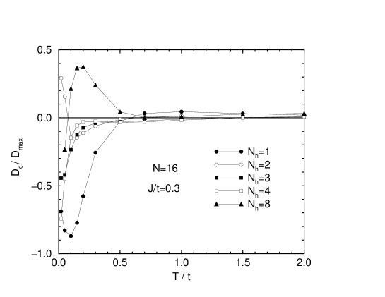
Figure 5.1: Normalized charge stiffness $D_{c}/D_{max}$ for various number on holes $N_{h}$ in a system with $N=16$ sites.

5.3 Single-hole mobility

It is expected that at low doping the conductivity scales linearly with doping, hence it is meaningful to introduce the dynamical mobility $\mu(\omega)$ which is a single-hole property

$$\sigma(\omega)=e_{0}c_{h}\mu(\omega),$$ (5.11)

but still highly nontrivial for a Mott or an AFM insulator.

The most conclusive theoretical results (in 2D or higher D systems) have been so far obtained for a problem of a single mobile hole introduced into a reference insulator. Brinkman and Rice (1970) solved the problem for $J=0$ within RPA. They pointed out of an essentially incoherent hole motion and evaluated the d.c. mobility $\mu_{0}(T)$, exhibiting $\mu_{0}\propto T$ for $T>t$. $\mu(\omega)$ within RPA (Rice and Zhang 1989) shows an incoherent motion, resulting in a slow non-Drude fall-off $\mu(\omega)\propto 1/\omega$ for larger $\omega$. The RPA has been recently justified and applied more rigorously for infinite-D lattices (Metzner et al. 1992). An analogous approach is the evaluation of frequency moments of $\mu(\omega)$, starting at $T\gg t$, as applied to the $J=0$ problem by Ohata and Kubo (1970). On the other hand, $\mu(\omega)$ at $T=0$ has been in recent years well established by numerical studies of small systems via the ED method (Sega and Prelovšek 1990, Dagotto 1994). Nevertheless there are important unsolved questions even for the single-hole problem. Is $\mu(\omega)$ on a planar lattice qualitatively and quantitatively well described within the RPA, at least for $T>t$ ? Which are new qualitative dynamical features at $T<t$, both for the $J=0$ and the $J>0$ case ?

Results for $\mu(\omega)$ at $J=0$, obtained via the FTLM by Jaklič and Prelovšek (1995c), show an overall agreement with the RPA. However, in contrast to the smooth RPA curve the actual $\mu(\omega)$, evaluated at $T\gg t$, seems to be nonanalytical, i.e. it shows a cusp at $\omega=0$. The phenomenon seems to be characteristic for $J=0$, but not for $J>0$. $\mu(\omega)$ for $J=0$ retains its high-$T$ form for all $T>t$, but changes qualitatively for $T<t$. Here the central peak due to the formation of the FM polaron (Nagaoka 1966) starts to emerge at low $\omega$, and the incoherent broad background steadily vanishes on approaching $T\rightarrow 0$.

We are more interested in the AFM case, as shown in Fig. 5.2. For $T>t$ the spin background is disordered and the mobility retains the high-$T$ form $\mu(\omega)\propto\beta$, leading to $\mu_{0}\propto 1/T$. As seen from Fig. 5.2, there is a qualitative change already in the regime $J<T<t$. Namely, it appears that here $\mu(\omega)$ has a weaker $T$-dependence. For $T\rightarrow 0$ we are however approaching a nontrivial response of an AFM polaron, which has been analyzed numerically by several authors. At $T=0$ one expects in $\mu(\omega)$ for $\omega\to 0$ a coherent response of an AFM polaron with an enhanced mass, but also a nonvanishing incoherent part at $\omega>J$ (Sega and Prelovšek 1990, Dagotto 1994). The latter component seems to have a nontrivial internal structure being related to the mid-infrared peak, as realized also in Fig. 5.2 for the lowest $T=0.1~{}t$.

Figure 5.2: Dynamical mobility $\mu(\omega)$ for a single hole in an AFM at various $T$.

From $\mu(\omega)$ one can extract the d.c. mobility $\mu_{0}$. Results for $J=0.3~{}t$ and $J=0$ are presented in Fig. 5.3, with the RPA ($J=0$) result for comparison. While for $T>2t$ we see the high-$T$ result $\mu_{0}\propto 1/T$ for both $J$, we get for the AFM case a nontrivial $\mu_{0}\sim const$ within the regime $J<T<t$. It is plausible that $J>0$ reduces $\mu_{0}$ as follows also from the frequency-moment analysis at $T\gg t$ (Jaklič and Prelovšek 1995c), indicating that in an AFM the hole motion is more frustrated leading to stronger scattering. As one can realize from Fig. 5.2, it is hard to get meaningful results for $T<J\sim T_{fs}$, since in this regime the central QP peak is essentially undamped. This is an indication that we are already dealing with finite-size effects, as discussed in Sec. 5.2, and the mean free path is beyond our system size $l_{s}>L$. Naively one would expect from Fig. 5.3 that in the regime $T<J$ $\mu_{0}$ would increase with decreasing $T$, whereby the scattering of the QP (AFM polaron) should be on thermally excited magnons. There are however unsolved problems with such a description. In an AFM the QP dispersion (Kane at al. 1989, Martinez and Horsch 1991) is strongly renormalized and is effectively narrower than the magnon one, hence it seems hard to find appropriate allowed scattering processes. These questions become important when discussing the relation of calculated $\mu_{0}$ to the resistivity of cuprates at low doping, as discussed in Sec. 5.5.

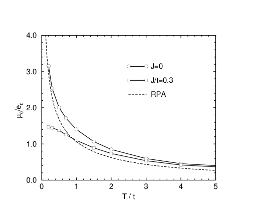
Figure 5.3: D.c. mobility $\mu_{0}$ vs. $T$ for $J=0$ and $J/t=0.3$. The RPA result is shown for comparison.

5.4 Optical conductivity at finite doping

Even more challenging questions appear at finite hole doping. Whereas at low doping one could treat the transport within the semiconductor-like model of independent QP - AFM polarons, this concept fails even for a moderate $c_{h}\gtrsim 0.1$ due to the overlap between extended spin deformations around holes. Alternative indications for such a phenomenon have been already discussed in Sec. 4 in connection with $c_{h}(\mu_{h})$.

Since in a planar system we are evaluating the sheet conductivity $\sigma(\omega)$ it is convenient to discuss at finite doping the dimensionless quantity $\bar{\sigma}=\sigma\rho_{0}$, where $\rho_{0}=\hbar/e_{0}^{2}=4.1k\Omega$ is the universal 2D sheet resistance. Such a quantity has an additional meaning since it makes a direct contact with the theory of localization, where $\bar{\sigma}_{0}\sim\bar{\sigma}_{min}$ is a characteristic marginal value associated with the 2D minimum metallic conductivity (Mott and Davis 1979). The value of $\bar{\sigma}_{min}$ and its relevance is however controversial, and it ranges from $\bar{\sigma}_{min}=0.1$ (Mott and Davis 1979) to $\bar{\sigma}_{min}\sim 0.5$ found in experiments (Mandrus et al. 1991) as a borderline between insulating and conducting cuprates at low $T$.

5.4.1 Intermediate doping

Let us go straight to results at the intermediate (optimum) doping, where we can reach lowest $T_{fs}$. Instead of $\sigma(\omega)$ it is more instructive to present the current correlation function $C(\omega)$, equation (5.1). To avoid the ambiguities with an additional smoothing, we plot the corresponding integrated spectra

$$I_{C}(\omega)=\int_{0}^{\omega}C(\omega^{\prime})d\omega^{\prime}.$$ (5.12)

In Fig. 5.4 we present $I_{C}(\omega)$ for $c_{h}=3/16$, for various $T\leq t$. Spectra reveal several remarkable features (Jaklič and Prelovšek 1995b):

(i) For $T\leq J$ spectra $I_{C}(\omega)$ are essentially independent of $T$, at least for available $T>T_{fs}$.

(ii) Simultaneously the slope of $I_{C}(\omega<2~{}t)$ is nearly constant, i.e. we find $C(\omega)\sim C_{0}$ in a wide $\omega$ range. At the same time $C_{0}$ is only weakly dependent on $J$ as tested for $J/t=0.2-0.6$.

(iii) Even for higher $T>J$ the differences in the slope $C_{0}$, as also in $I_{C}(\infty)$, appear as less essential. Note that for $T\gg t$ we know exactly $I_{C}(\infty)=\pi t^{2}c_{h}(1-c_{h})$ (Jaklič and Prelovšek 1995c).

Figure 5.4: Integrated current correlation spectra $I_{C}(\omega)$ at $c_{h}=3/16$ for different $T\leq t$.

We conclude that $C(\omega<2~{}t)\sim C_{0}$ implies a simple universal form (Jaklič and Prelovšek 1995b),

$$\sigma(\omega)=C_{0}e_{0}^{2}{1-e^{-\beta\omega}\over\omega}.$$ (5.13)

Such a $\sigma(\omega)$ shows a nonanalytic behaviour at $\omega\rightarrow 0$, starting with a finite slope. This is already an indication that $\sigma(\omega)$ is not consistent with the usual Drude form, but rather with a marginal concept (Varma et al. 1989) where the only $\omega$ scale is given by $T$. It is also remarkable that the form (5.13) trivially reproduces the linear law $\rho\propto T$ as well as the non-Drude fall-off at $\omega>T$. It is evident that the expression (5.13) is universal containing the only parameter $C_{0}$ as a prefactor.

Experimental results and theoretical considerations are often discussed in terms of the $\omega$-dependent relaxation time $\tau$ and the effective mass $m^{*}$. These can be uniquely introduced via the complex $\tilde{\sigma}(\omega)$ and the corresponding memory function $M(\omega)$ (Götze and Wölfle 1972),

$$\tilde{\sigma}(\omega)={ie_{0}^{2}{\cal S}\over\omega+M(\omega)},\qquad\qquad{\cal S}=-\langle H_{kin}\rangle/2N,$$ (5.14)

and

$${1\over\tau(\omega)} = {M^{\prime\prime}(\omega)\over 1+M^{\prime}(\omega)/\omega},$$

$${m^{*}(\omega)\over m_{t}} = {2c_{h}t\over{\cal S}}\left(1+{M^{\prime}(\omega)\over\omega}\right),$$ (5.15)

where $m_{t}=1/2ta_{0}^{2}$ is the bare band mass. Using relations (5.14),(5.15) one can formally rewrite $\tilde{\sigma}(\omega)$ in the familiar Drude form

$$\tilde{\sigma}(\omega)={ic_{h}e_{0}^{2}\over m^{*}(\omega)[\omega+i/\tau(\omega)]}.$$ (5.16)

Employing the equation (5.16) we evaluate both $\tau(\omega)$ and $m^{*}(\omega)$ from known $\tilde{\sigma}(\omega)$. Results for $c_{h}=3/16$, corresponding to Fig. 5.4, are presented in Fig. 5.5.

It follows from Fig. 5.5a, but even more directly from the form (5.13), that in the regime $T\lesssim J$ and $\omega<t$ we can describe the behaviour of $1/\tau$ with a linear law

$$\tau^{-1}=2\pi\lambda(\omega+\xi T),\qquad\lambda\sim 0.09,~{}~{}~{}\xi\sim 2.7~{}.$$ (5.17)

This dependence falls within the general framework of the MFL scenario. It is however not the form (2.3) proposed originally (Varma et al. 1989, Littlewood and Varma 1990), but rather the one (2.4) deduced from experiments in cuprates (El Azrak et al. 1995, Baraduc et al. 1995). It should be however stressed that the asymptotic form (5.17) does not allow for any free parameter, i.e. constants $\lambda$ and $\xi$ are universal and independent of any model parameters, whereas within the MFL proposal $\lambda$ is an adjustable parameter while $\xi=\pi$.

 

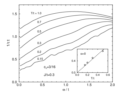
Figure 5.5: (a) Inverse relaxation time $1/\tau$, and (b) mass enhancement $m^{*}/m_{t}$ vs. $\omega$, for $c_{h}=3/16$ and different $T$. The insert in a) shows the $T$-dependence of $1/\tau(0)$.

It should be also mentioned that the universal dynamics, as described by the equation (5.13), does not seem to be restricted only to the particular case of doped AFM, but has a wider applicability, e.g. it has been recently established also in ladder systems (Tsunetsugu and Imada 1997).

5.4.2 Underdoped and overdoped regime

Let us turn to the discussion of results at other dopings $c_{h}$. Results for $c_{h}=4/16$ (Jaklič and Prelovšek 1995c) are in all aspects very similar to the $c_{h}=3/16$ case. We show in Figs. 5.6 analogous $I_{C}(\omega)$ for underdoped $c_{h}=2/18$, as well as for overdoped $c_{h}=7/16$. One feature common to all $c_{h}$ considered (including $N_{h}=1$) is the non-Drude behaviour for $\omega>t$. This confirms the belief that the incoherent motion of holes, dominating the high-$\omega$ response as described e.g. within the RPA (Rice and Zhang 1989), can remain a valid concept even at large doping $c_{h}<0.5$.

 

Figure 5.6: $I_{C}(\omega)$ for (a) $c_{h}=2/18$, and (b) $c_{h}=7/16$, for different $T$.

Otherwise it is harder to make conclusions on the most interesting low-$(\omega,T)$ regime, both for the underdoped as well as for the overdoped case. For $c_{h}=2/18$ we note that in contrast to Fig. 5.4 the low-$\omega$ slope is not constant at $T<J$ but is still gradually decreasing with $T$. This results in a modified variation of the d.c. conductivity $\sigma_{0}\propto 1/T^{1-\eta}$ with $\eta>0$, hence also in a sublinear $\rho_{0}\propto T^{1-\eta}$. On the other hand we see already for $T=0.1~{}t$ a drop of $I_{C}(\infty)$ (closely related to the sum rule) which can be interpreted with a significant persistent (nonscattered) current in a system with p.b.c. The latter emerges as the coherent part with $D_{c}>0$ according to the equation (5.3), not taken into account in the presented $I_{C}(\omega)$. While we cannot say much on the current relaxation of such a coherent part, it is plausible that an increase in the coherence should decrease the resistivity $\rho_{0}$, as found in underdoped cuprates below the crossover $T^{*}$. Otherwise results in Fig. 5.6a are close to curves for a single hole in an AFM, Fig. 5.2, with the difference that in the latter case $T^{*}$ appears even higher.

In the overdoped case in Fig. 5.6b $I_{C}(\infty)$ starts to deviate from a constant already for $T\lesssim J$. At $T<J$ a sharp increase of an unscattered current appears, so we are unable to speculate on a possible onset of more LFL-like $\rho\propto T^{2}$.

5.4.3 Effects of the next-nearest-neighbour hopping

It is a relevant question whether the anomalous but universal behaviour of $\sigma(\omega)$ found at the intermediate doping is spoiled by possible additional terms, e.g. by the introduction of the n.n.n. hopping $t^{\prime}$ term (2.7), invoked often to obtain a realistic description of cuprates. When considering the effect of $t^{\prime}$ it is important to realize that at finite doping $t^{\prime}>0$ tends to stabilize the AFM ordering while $t^{\prime}<0$ destabilizes it and tends toward a Nagaoka-type FM state (Bonča and Prelovšek 1989).

Results for $I_{C}(\omega)$ at $t^{\prime}\neq 0$ are presented in Fig. 5.7. We choose rather modest $|t^{\prime}/t|=0.2$, still quite a pronounced effect on $I_{C}(\infty)$ is evident. We should note that in this case also generalized sum rules, following equations (5.5) and (5.8), apply. On the other hand, the low-$\omega$ part is not changed essentially. For $t^{\prime}/t=0.2$ we note again an universal behaviour according to the form (5.13). Deviations at lowest $T$ are somewhat larger for $t^{\prime}/t=-0.2$. A possible interpretation of these results is that $t^{\prime}\neq 0$ moves the system effectively away from the starting doping regime, i.e. drives an optimum system either towards the underdoped or to the overdoped regime.

Figure 5.7: $I_{C}(\omega)$ for $c_{h}=3/18$ and the n.n.n. hopping: a) $t^{\prime}/t=0.2$, and b) $t^{\prime}/t=-0.2$, for different $T$.

5.5 Resistivity

Finally, we display results for the d.c. resistivities $\rho(T)$, as extracted from $\sigma(\omega\rightarrow 0)$. The extrapolation $\omega\rightarrow 0$ is straightforward at higher $T$. It becomes somewhat more delicate on approaching $T\sim T_{fs}$ due to the appearance of more pronounced structures and $D_{c}\neq 0$. Actually, we can evaluate $\sigma_{0}$ either from $\sigma(\omega)$ which involves some smoothing, or from the slope of $I_{C}(\omega\sim 0)$ which seems to be more reliable.

In Fig. 5.8 we present results for $\rho(T)$ at various $c_{h}$ for $J/t=~{}0.3$, and in comparison also for $J=0$. We first notice that at $T>t$ calculated $\rho(T)\propto T$. The slope at $T>t$ is nearly independent of $J$, the main effect of finite $J>0$ being the upward shift of $\rho(T)$ curves. The shift also decreases as doping is increased, since it is plausible that the effect of $J$ nearly vanishes in the overdoped regime $c_{h}>0.3$. The slope at $T>t$ can be approximately given (for $c_{h}<0.25$) as $d\rho/dT\sim\zeta\rho_{0}k_{B}/c_{h}t$ with $\zeta\sim 0.4$. This value confirms the relevance ot the RPA (Brinkman and Rice 1970), which yields for a square lattice $\zeta\sim 0.72$.

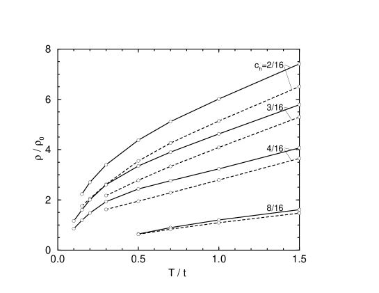
Figure 5.8: Resistivity $\rho$ vs. $T$ at different $c_{h}=N_{h}/N$ for $J=~{}0.3~{}t$ (full lines) and $J=0$ (dashed lines).

One could expect essential changes in the regime $T\lesssim J$. It is evident from Fig. 5.8 that at the intermediate doping $0.15<c_{h}\lesssim 0.25$ the curve $\rho(T)$ changes the slope at $T\sim J$. Nevertheless $\rho(T<J)$ is still linear in $T$, as emerges also from the observed universal form (5.13). As discussed in Sec. 5.4.2, the underdoped systems as $c_{h}=2/16$ show already deviations from the universality (5.13). Two effects should be mentioned. In the regime where our analysis is fully applicable and $l_{s}<L$ we find sublinear $\rho(T)\propto T^{1-\eta}$, which could be interpreted also as $\rho(T)\sim A+BT$ with a positive intercept $A>0$. On the other hand, the appearance of $D_{c}\neq 0$ in our results seems to be closely related to another scale $T\sim T^{*}$ where a kink of $\rho(T)$ appears. It should be also noted that the introduction of the n.n.n. hopping $t^{\prime}\neq 0$ does not change qualitative conclusions.

5.6 Relation to experiments

In 2D $\sigma$ is naturally expressed in terms of the universal constant $\rho_{0}=\hbar/e_{0}^{2}$. The corresponding 3D conductivity of a stack of 2D conducting sheets with an average distance $\bar{c}$ is given instead by $\sigma_{3D}=\sigma/\bar{c}$. For comparison with experiments we reduce the 3D measured values to the 2D conductivities for three different cuprates at intermediate doping, i.e. LSCO with $x=0.2$ (Uchida et al. 1991), Bi₂Sr₂CaCu₂O₈ (BISCCO) (Romero et al. 1992), and YBCO (Cooper et al. 1993). Experimental results are taken at relatively low temperatures $T<200~{}K$, i.e. at $T<T_{fs}$ below the sensitivity of our small-system calculations. It is an open experimental question whether spectra reduced in this way are really universal, i.e. whether they depend only on the hole concentration $c_{h}$ in conducting CuO₂ layers or other details of material structure are still important. Moreover, effective $c_{h}$ for presented materials are known only approximately, except for LSCO where $c_{h}\sim x$, i.e. it is estimated that $c_{h}\sim 0.23$ for BISCCO and YBCO (Batlogg et al. 1994).

Taking into account this uncertainty calculated spectra $\sigma(\omega)$ for $c_{h}=3/16$ are in a quantitative agreement with measurements, as seen in Fig. 5.9, where the energies are expressed in eV using $t=0.4$ eV. We note also that at high $\omega\gtrsim 1~{}eV$ the fall-off of calculated $\sigma(\omega)$ is faster than that of measured ones. This could be explained by the emerging contribution of transitions to excited (charge transfer or upper Hubbard band) states not taken into account within the $t-J$ model, but clearly identified experimentally (Uchida et al. 1991).

Figure 5.9: Sheet conductivities $\sigma(\omega)$ for various $T/t$, in comparison with measurements in different cuprates. Experimental results refer to $T<200~{}K$.

It should be noted that also calculated $\tau^{-1}(\omega)$ and corresponding parameters $\lambda$ and $\xi$, as defined by the equation (5.17) are close to the experimental ones. E.g., an analysis in a wide frequency range $\omega<1000~{}$cm^-1 presented for YBCO and BISCCO data by El Azrak et al. (1994) yields $\lambda\sim 0.11$, while a broader class of optimally doped materials is consistent with $0.1<\lambda<0.15$ (Baraduc et al. 1995). A recent investigation (Startseva et al. 1997) in a narrower $\omega$ range obtains for an overdoped LSCO ($x=0.22$) similar values $0.06<\lambda<0.08$.

Also $m^{*}/m_{t}$ in Fig. 5.5b qualitatively agrees with experimental findings (Romero et al. 1992, El Azrak et al. 1994, Tanner and Timusk 1992, Cooper et al. 1993). For a quantitative comparison we should note that by lowering $T$ to experimentally investigated values we expect the increase of $m^{*}$ at low $\omega$. On the other hand, assuming realistic values $a_{0}=0.38~{}{\rm nm}$ and $t=0.4~{}{{\rm eV}}$ we should also take into account that $m_{t}\sim 0.6~{}m_{0}$.

In Fig. 5.10 we compare calculated resistivities to the measured ones. It should be pointed out that there is a restricted $T$ window where a comparison could be made since $T_{fs}\sim 450K$, whereby at $T\sim T_{fs}$ also finite-size effects start to influence our analysis. Nevertheless, for the intermediate doping $c_{h}\sim 0.2$ our $\rho(T)$ results match quantitatively well experimental ones for cuprates with comparable hole concentrations, i.e. for BISCCO, YBCO and LSCO with $x=0.15$ (Takagi et al. 1992, Batlogg et al. 1994, Iye 1992).

Figure 5.10: Sheet resistivities $\rho(T)$ for various dopings (full lines) in comparison with measurements in LSCO with $x=0.15$ (dotted), BISCCO (dashed), and YBCO (dash-dotted).

Turning to underdoped materials, there are certain features which are reproduced in our results. First, our $\mu(\omega)$ for a single hole, see Fig. 5.2, as well as several $T=0$ numerical studies (Sega and Prelovšek 1990, Dagotto 1994) indicate an existence of a mid-infrared peak in $\sigma(\omega)$, being a signature of magnon excitations in a spin background with a longer range AFM order. This feature has been seen in experiments in LSCO (Uchida et al. 1991 ), although its appearance in other materials is controversial. We also reproduce the observation that at moderate doping $c_{h}>0.1$ the resistivity essentially scales as $\rho\propto 1/c_{h}$. An unproportional increase of $\rho$ at low doping $c_{h}<0.1$, as deduced when comparing values in Fig. 5.10 with single-hole mobilities in Fig. 5.3, is as well consistent with experiments, e.g. for LSCO with $x<0.1$ (Takagi et al. 1992).

6 Magnetic Properties

The static spin response and the spin dynamics in the undoped and doped AFM state in cuprates have been experimentally studied by the neutron scattering (see e.g. Shirane 1991), by NMR techniques (see e.g. Slichter 1994), as well by other methods.

Magnetic excitations in cuprates as measured by the neutron scattering reveal in insulating materials La₂CuO₄ (Keimer et al. 1992, Hayden et al. 1996) and YBa₂Cu₃O₆ (Rossat-Mignot et al. 1991) a remarkable agreement with the magnons within the planar Heisenberg AFM. On the other hand, a consistent description of magnetic properties of doped cuprates is still lacking. Nevertheless it is quite clear that the normal-state spin dynamics differs qualitatively from the one expected for LFL. In doped LSCO NMR and NQR spin-lattice relaxation time $T_{1}$ on Cu nuclei is generically nearly $T$ and doping independent in the normal state ($T>T_{c}$) (Imai et al. 1993), in contrast to the Korringa law $1/T_{1}\propto T$ in normal metals. Also, in the same regime the low-$\omega$ dynamical susceptibility in doped systems appears to be consistent with $\chi^{\prime\prime}(\omega)\propto\omega/T$ (Shirane 1991, Keimer et al. 1992, Sternlieb et al. 1993). Experimental investigations in recent years have been focused on underdoped materials, which show in the normal phase the emerging spin gap both in the NMR (Slichter 1994) and in the neutron scattering (Sternlieb et al. 1993), but also the appearance of charge stripes related to AFM domains (Tranquada et al. 1995). Since the latter phenomena appear only at lower $T$, hardly accessible in our studies, we shall comment them only briefly lateron.

Well understood theoretically is so far the isotropic quantum AFM, with the long-range order at $T=0$ (Manousakis 1991). For doped systems several phenomenological explanations (see Sec. 2.2) have been presented for magnetic properties. NMR and NQR data on the spin dynamics have been interpreted within the NAFL scenario (Millis et al. 1990, Millis and Monien 1992), where the $T$ dependence is attributed to the variation of the AFM correlation length $\xi(T)$. At low hole doping the mapping on the quantum critical scaling regime of the nonlinear sigma model, with the main ingredient $\xi\propto 1/T$, has been advocated by Sokol and Pines (1993). An alternative scenario for the low-$(\omega,T)$ behaviour is the MFL scenario (Varma et al. 1989, Littlewood and Varma 1991), where $\xi(T)$ is short and not crucially $T$-dependent.

Most reliable model results for magnetic properties of doped AFM have been obtained for static quantities by QMC studies of the Hubbard model and by the g.s. ED of the $t$-$J$ model (see Dagotto 1994), as well as by means of the HTE analysis (Singh and Glenister 1992a). Much less conclusive are results for the spin dynamics. While g.s. ED studies of the spin structure factor $S(\vec{q},\omega)$ (Tohyama et al. 1995, Eder et al. 1995) reveal quite an essential difference between $S(\vec{q},\omega)$ and corresponding charge spectra $N(\vec{q},\omega)$, they cannot give reliable conclusions for the low-$\omega$ behaviour. There have been only few attempts to address numerically dynamical properties at $T>0$ (Tohyama et al. 1993), prior to the application of the FTLM (Jaklič and Prelovšek 1995a, b). It should be reminded that most challenging questions (related to the normal state) refer to the dynamics at low $\omega$ and to the d.c. spin response in the strong correlation regime $J<t$ at low $T<J$.

6.1 Spin response

We consider the response of the electronic system to the time-dependent, spatially modulated magnetic field, which couples to the spin degrees of freedom via a Zeeman term

$$H^{\prime}=NM^{z}_{\vec{q}}B_{\vec{q}},\qquad M^{z}_{\vec{q}}=-{g\mu_{B}\over N}\sum_{i}e^{i\vec{q}\cdot\vec{R_{i}}}S_{i}^{z},$$ (6.1)

Within the linear response theory the magnetization response is given by

$$\delta\langle M^{z}_{\vec{q}}\rangle(\omega)=g^{2}\mu_{B}^{2}\chi(\vec{q},\omega)B_{\vec{q}}(\omega),$$ (6.2)

where

$$\chi(\vec{q},\omega) = i\int_{0}^{\infty}dt\;e^{i\omega t}\langle[S^{z}_{\vec{q}}(t),S^{z}_{-\vec{q}}(0)]\rangle,$$

$$S^{z}_{\vec{q}} = (1/\sqrt{N})\sum_{i}e^{i\vec{q}\cdot\vec{R}_{i}}S^{z}_{i}.$$ (6.3)

$\chi^{\prime\prime}(\vec{q},\omega)$ can be expressed with the dynamical spin structure factor $S(\vec{q},\omega)$

$$\chi^{\prime\prime}(\vec{q},\omega) = \pi(1-e^{-\beta\omega})S(\vec{q},\omega),$$

$$S(\vec{q},\omega) = {1\over\pi}{\rm Re}\int_{0}^{\infty}dt\;e^{i\omega t}\langle S^{z}_{\vec{q}}(t)S^{z}_{-\vec{q}}(0)\rangle.$$ (6.4)

$S(\vec{q},\omega)$ is the quantity directly evaluated within the FTLM, following the expression (3.41). Consequently the static structure factor and the static susceptibility can be evaluated,

$$S(\vec{q}) = \int_{-\infty}^{\infty}S(\vec{q},\omega)d\omega=\langle S^{z}_{\vec{q}}S^{z}_{-\vec{q}}\rangle,$$

$$\chi(\vec{q}) = \chi^{\prime}(\vec{q},0)=\frac{1}{\pi}{\cal P}\int_{-\infty}^{\infty}\frac{\chi^{\prime\prime}(\vec{q},\omega)}{\omega}d\omega.$$ (6.5)

6.2 Uniform spin susceptibility and Wilson ratio

The uniform case $\vec{q}=0$ is particular, since $S_{z}^{tot}$ is a conserved quantity. Then one can use for the uniform static spin-susceptibility $\chi_{0}$ the expression

$$\chi_{0}=\chi(\vec{q}=0)=\beta S(\vec{q}=0)=\frac{\langle(S_{z}^{tot})^{2}\rangle}{NT}.$$ (6.6)

The calculation reduces to the one involving only a thermodynamic average of a conserved operator, and an analysis analogous to the one used in Sec. 4 applies. This simplification allows for the consideration of larger systems, i.e. we calculate $\chi_{0}(T)$ for a system of $N=20$ sites in the range $0<c_{h}<0.3$, while for the undoped AFM (Heisenberg model) we reach $N=26$ (Jaklič and Prelovšek 1996).

Results at several $c_{h}$ are presented in Fig. 6.1. For $c_{h}=0$ our results agree with the HTE (Singh and Glenister 1992a) down to $T\sim 0.3~{}J$. In an AFM $\chi_{0}$ exhibits a maximum at $T=T^{*}\sim J$, which reflects the onset of the short range AFM order for $T<T^{*}$. Namely, at $T\to 0$ the longitudinal spin fluctuations in an ordered AFM gradually freeze out, while transverse ones remain constant, thus leading to a reduced $\chi_{0}(T\to 0)$.

Figure 6.1: Uniform susceptibility $\chi_{0}$ vs. $T$ at several $c_{h}$ in steps of 0.05 within a system of $N=20$ sites. $c_{h}=0$ is obtained for $N=26$.

For a finite doping $\chi_{0}$ is only weakly diminished for $T>J$, the reduction being due to a reduced number of spins in the system. On the other hand, the qualitative change appears for $T<J$. The maximum $T^{*}$ gradually shifts to lower $T$ with doping and finally disappears at $c_{h}>0.15$. In the overdoped regime $c_{h}\gtrsim 0.15$ we observe a monotonous Pauli-like $\chi_{0}$ for $T<0.2~{}t$, which could signify an onset of a low-$T$ behaviour consistent with the LFL picture. Still up to $c_{h}>0.6$ we do not find the usual LFL behaviour $\chi_{0}(T)={\rm const}$, but rather $\chi(T)$ still increases nearly linearly on lowering $T\to 0$.

Obtained results are quite consistent with experiments on cuprates. First, $\chi_{0}$ at $T\to 0$ increases with doping as found in LSCO (Johnston 1989, Torrance et al. 1989) and the existence of a maximum of $\chi_{0}(T)$ at $T^{*}(c_{h})$ in underdoped cuprates has been interpreted in terms of a pseudogap scale (Batlogg et al. 1994). It is evident from our results that such a pseudogap is inherent within the $t$-$J$ model and is intimately related to the short range AFM order. It is remarkable that in the model this feature disappears, i.e. $T^{*}\to 0$, just at a similar (optimum) doping $c_{h}\sim 0.15$ as in cuprates (Batlogg et al. 1994). Note also that the unusual linear increase of $\chi_{0}(T\to 0)$ in the overdoped regime, see Fig. 6.1 for $c_{h}=0.2$, seems to be well consistent with experimental results in overdoped LSCO (Loram et al. 1996).

Here we can also comment on the ratio $W=(g^{2}\mu_{B}^{2}\chi_{0})/\gamma$ where $\gamma=C_{V}/T$. It is used as a test for the concept of nearly free QP, where one expects $W_{0}={1\over 3}(\pi k_{B}/\mu_{B})^{2}$. The meaningful measure is thus the Wilson ratio $R_{W}=W/W_{0}$ being often studied in correlated systems, in particular in connection with heavy-fermion metals. In our case it is convenient to perform the test on $s$ directly by defining $\tilde{\gamma}=s/T$ (see also Loram et al. 1996). In our notation the dimensionless Wilson ratio can be expressed as

$$R_{W}={4\pi^{2}\over 3}{(k_{B}T/t)(\chi_{0}t)\over s/k_{B}}.$$ (6.7)

We can now easily evaluate $R_{W}$ by comparing results in Fig. 4.3a with Fig. 6.1 and results are shown in Fig. 6.2. It is quite striking that in the intermediate regime $0.1\lesssim c_{h}\lesssim 0.2$ at low $T\ll J$ we find values, very close to the free fermion one, i.e. $R_{W}=1$. In the overdoped regime calculated values are somewhat larger, but still $R_{W}<2$. The same seems to be the case for the underdoped case $c_{h}=0.05$, where results at lowest $T$ should be taken with care. With increasing $T$ also $R_{W}$ is increasing and seems to reach quite a wide plateau for $T\gtrsim J$ with $R_{W}\sim 2$.

Figure 6.2: Wilson ratio $R_{W}$ vs. T at several $c_{h}$.

This finding is quite puzzling since clearly doped AFM are far from a simple LFL, and apparently even further from free fermions. Note however that experimental results also yield $R_{W}\sim 1$, both for LSCO and YBCO (Loram et al. 1996). Moreover, the same experiments indicate that $s\propto T\chi_{0}$ in a wide range of $T$ and doping, so $R_{W}$ as defined in the equation (6.7) is nearly $T$ independent.

6.3 Spin structure factor and dynamical susceptibility

Let us first discuss $S(\vec{Q},\omega)$ spectra at the AFM wavevector $\vec{Q}=(\pi,\pi)$, where the spin response is most pronounced. In Fig. 6.3 we present results at fixed $T=0.2~{}t<J$, but various dopings $c_{h}$ (Jaklič and Prelovšek 1995a). It should be noted that $S(\vec{Q},\omega)$ is not symmetric around $\omega=0$, hence a maximum appears in general at $\omega>0$. The most interesting feature in Fig. 6.3 is the qualitative change of spectra on doping. At low doping $c_{h}<0.12$ we see that $S(\vec{Q},\omega)$ is dominated by a single central peak, i.e. we are observing mainly the AFM spin fluctuations of a Heisenberg model. The main effect of holes is to reduce the AFM correlation length, and consequently the intensity of the central peak.

Figure 6.3: Spin structure factor $S(\vec{Q},\omega)$ at fixed $T=0.2~{}t<J$ and different dopings $c_{h}$.

In the intermediate regime $0.12<c_{h}<0.3$ a high-frequency component with $\omega\gtrsim t$ emerges, coexisting with the remaining low-$\omega$ fluctuations. It is quite plausible to attribute the high-$\omega$ dynamics to the free-fermion-like component of the correlated system, in particular since it appears to be quite independent of $J$ (provided that $J<t$). Although this observation is consistent with previous studies (Tohyama et al. 1993, Putikka et al. 1994), the coexistence of spin-fluctuation and free-fermion timescales at the intermediate doping has been clearly established only by using the FTLM (Jaklič and Prelovšek 1995a). Namely, it is harder for other methods, e.g. within the HTE method, to resolve coexisting different timescales. The dual character is a crucial property, since the free-fermion part determines to large extent static spin correlations $S(\vec{q})$ through the relation (6.5), as well as the electron (charge) density correlations $N(\vec{q})$, discussed in Sec. 8.1. The latter have been in fact interpreted in terms of a quasi FS (Putikka et al. 1994). On the other hand the low-$\omega$ spin dynamics dominates dynamical and static spin susceptibilities, i.e. $\chi^{\prime\prime}(\vec{q},\omega)/\omega$ and $\chi(\vec{q})$, hence the low-$\omega$ neutron scattering and NMR processes. It is also evident that in the overdoped regime $c_{h}>0.3$ the low-frequency component is disappearing and the free-fermion-like fluctuations tend to exhaust the spectra. $S(\vec{Q},\omega)$ is nevertheless quite distinct from the one for free fermions, even at $c_{h}\sim 0.5$.

Before we present results for general ${\vec{q}}\neq\vec{Q}$, let us discuss the AFM correlation length $\xi(T)$. One can evaluate $\xi(T)$ from the static real space correlations $S(\vec{r})$, corresponding to $S(\vec{q})$, i.e.

$$\xi^{2}=\frac{1}{4S(\vec{Q})}\sum_{i}|\vec{r}_{i}|^{2}\exp(i\vec{Q}\cdot\vec{r}_{i})S(\vec{r}_{i}).$$ (6.8)

In the most interesting regime $c_{h}=0.1-0.3$ we find that $\xi$ is short, typically $\xi\sim 1$, governed by correlations at $r_{i}=1$. It increases less than $30\%$ between $T=J$ and $T=J/3$. This finding (Jaklič and Prelovšek 1995a) is well in agreement with the HTE studies (Singh and Glenister 1992a), with the QMC results for the Hubbard model (Furukawa and Imada 1992) as well as with values $\xi(T=0)$ obtained via the ED within the $t-J$ model (Dagotto 1994). Similar values for $\xi$ can be extracted also considering our results for static $\chi(\vec{q})$, although results are less conclusive at low $T\sim T_{fs}$.

In recent years experiments in cuprates have shown the possibility of longer range (or even long range) spin correlations with $\vec{q}\neq\vec{Q}$ (Tranquada et al. 1995, Hayden et al. 1996). This has been related either to an incommensurate spin order or to the appearance of charge stripes. Such structures are well possible within the $t$-$J$ model (Prelovšek and Zotos 1990, White and Scalapino 1997b) although it is controversial whether they are stable in the most interesting regime $J\ll t$. Nevertheless we do not expect to resolve them in our calculations for $J/t=0.3$, since they could possibly appear only for $T<T_{fs}$ and could be also missed due to particular clusters which do not prefer expected orderings.

Let us turn to dynamical susceptibilities. Fig. 6.4 displays $\chi^{\prime\prime}(\vec{q},\omega)/\omega$ for fixed $c_{h}=3/16$, but various $T$ and nonequivalent $\vec{q}$. Note that on a $4\times 4$ lattice $\vec{q}=(0,\pi)$ and $\vec{q}=(\pi/2,\pi/2)$ are equivalent. In contrast to Fig. 6.3, high-$\omega$ features are now suppressed. Also, the free-fermion-like component is well separated from the low-$\omega$ part only for $\vec{q}\sim\vec{Q}$, where one expects a gap in the response of free fermions with a well defined FS. For other $\vec{q}$ the free-fermion contribution persists at larger $\omega>J$ in the form of a long tail, while in the low-$\omega$ regime it merges with the spin contribution.

Figure 6.4: $\chi^{\prime\prime}(\vec{q},\omega)/\omega$ at $c_{h}=3/16$ for nonequivalent $\vec{q}$ and different $T$: $T/t=0.1$ (full line), $0.2$ (dashed line), $0.3$ (dash-dotted line), and $0.5$ (dotted line).

The most striking feature of Fig. 6.4 is the strong $T$ dependence of the low-$\omega$ spectra, whereas the AFM correlation length $\xi$ has been found to be only weakly $T$ dependent. This conclusion on $\chi^{\prime\prime}(\vec{q},\omega)/\omega$ seems to hold within the correlation regime $|\vec{q}-\vec{Q}|<\xi^{-1}$, where also $\chi(\vec{q})\sim\chi(\vec{Q})$. The relevant volume in the $\vec{q}$ space clearly increases on doping and exhausts for $c_{h}=3/16$ already the substantial part of the Brillouin zone. The variation at low $\omega$ appears to follow,

$$\chi^{\prime\prime}(\vec{q},\omega)/\omega\propto 1/T,\qquad\omega<T<J,$$ (6.9)

or equivalently, from the relation (6.4) $S(\vec{q},\omega)$ is nearly $T$ and $\omega$ independent in the same regime. On the other hand, at the same doping scaling does not hold for $\vec{q}$ outside the correlation volume, e.g. for $\vec{q}=(0,\pi/2)$ in Fig. 6.4, where $\chi^{\prime\prime}(\vec{q},\omega)/\omega$ is approximately $T$ independent as expected within the LFL.

Spectra discussed above have as a direct consequence the $T$ variation of the static $\chi(\vec{q})$ for $T<J$. We observe a pronounced $T$ dependence, e.g. $\chi(\vec{q})\propto 1/T$ in a wide regime $J/3<T<t$ for all $q$ within the correlation regime. It should be however noted that we are quite restricted in the range of $T/J$, so that more quantitative conclusions on a possible power-law (or logarithmic) variation with $T$ are not feasible.

6.4 Local spin dynamics

In order to describe properly the spin correlation function $S(\vec{q},\omega)$ it is very helpful to consider the local spin correlation function $S_{L}(\omega)$ and its symmetric part $\bar{S}(\omega)$ (Jaklič and Prelovšek 1995b),

$$S_{L}(\omega) = {1\over N}\sum_{\vec{q}}S(\vec{q},\omega),$$

$$\bar{S}(\omega) = S_{L}(\omega)+S_{L}(-\omega)=(1+e^{-\beta\omega})S_{L}(\omega).$$ (6.10)

It should be noted that $S_{L}(\omega)$ and the related susceptibility $\chi_{L}(\omega)$ have been directly measured in cuprates by the neutron scattering (Shirane 1991), while the NMR relaxation on ⁶³Cu effectively yields the information on $S_{L}(\omega\rightarrow 0)$, as discussed in Sec. 6.5. An important restriction on $\bar{S}(\omega)$ is the sum rule following from the equation (6.5),

$$\int_{0}^{\infty}\bar{S}(\omega)d\omega=\langle(S_{i}^{z})^{2}\rangle={1\over 4}(1-c_{h}).$$ (6.11)

When we perform the calculation of $\bar{S}(\omega)$ we omit the singular $\vec{q}=0$ term in the summation (6.10), so the sum rule (6.11) serves as an useful test. In Fig. 6.5 we display $\bar{S}(\omega)$ for different dopings $c_{h}=1/20$ and $3/16$, and several $T$ in the range $0.1\leq T/t\leq 0.7$ (Jaklič and Prelovšek 1995b). It is immediately evident that $\bar{S}(\omega)$ at the optimum doping $c_{h}=3/16$ is essentially $T$ independent in a wide $T$ range, although one crosses the exchange-energy scale $T\sim J$.

Figure 6.5: Local spin correlation function $\bar{S}(\omega)$ for $c_{h}=1/20$ and $c_{h}=3/16$, and different $T$.

For the underdoped case $c_{h}=1/20$ as well as for the undoped AFM the behaviour is analogous for higher $T>T_{0}\sim 0.7~{}J$. Deviations appear at $T<T_{0}$, leading at $T\to 0$ to a decrease and to a flattening of $\bar{S}(\omega<2J)\sim const$, whereby a weak enhancement of $\bar{S}(\omega>2J)$ is then required by the sum rule. At least this regime of essentially pure Heisenberg model is well understood theoretically. The behaviour at $T>T_{0}$ is consistent with the quantum critical regime within the AFM, whereas for $T<T_{0}$ the renormalized classical regime applies (Chakravarty et al. 1989). In the latter regime we are dealing with longer range AFM correlations $\xi\gg 1$, hence $\bar{S}(\omega)$ is essentially that of an ordered AFM where the simple magnon picture leads in 2D to $\bar{S}(\omega<2J)\sim const$.

In Fig. 6.6 we follow the doping dependence of $\bar{S}(\omega)$ at fixed $T=0.2~{}t<J$. For convenience we plot again the integrated spectra, in analogy to the equation (5.12),

$$I_{S}(\omega)=\int_{0}^{\omega}\bar{S}(\omega^{\prime})d\omega^{\prime}.$$ (6.12)

For chosen $T$ results are again most reliable at the intermediate doping. The most striking message is that the initial slope of $I_{S}(\omega)$ and consequently $S_{L}(\omega\rightarrow 0)$ is nearly doping independent for $0\leq c_{h}\leq 0.25$, as well as $T$ independent at the intermediate doping. Only in the overdoped systems with $c_{h}>0.25$ the low-$\omega$ behaviour changes qualitatively, where the low-$\omega$ contribution is strongly suppressed as expected in a (more) normal FL. In a pure Heisenberg model the spin dynamics is nearly exhausted in the range $\omega<3J$ with excitations being magnons. On the other hand, at the intermediate doping $\bar{S}(\omega)$ decreases smoothly up to $\omega\sim 4t$, this being a consequence of the free-fermion-like component. Still up to $c_{h}\sim 0.3$ the dominant scale of spin fluctuations remains related to $J$.

Figure 6.6: Integrated spin correlation spectra $I_{S}(\omega)$ at fixed $T=0.2~{}t$ and different $c_{h}=N_{h}/N$.

Using equations (6.4) and (6.10) we finally note that the $T$-independent $\bar{S}(\omega)$ leads to the universal form

$$\chi^{\prime\prime}_{L}(\omega)={1\over\pi}\tanh\left({\omega\over 2T}\right)\bar{S}(\omega),$$ (6.13)

where the $T$ dependence is only in the thermodynamic prefactor. It follows from the equation (6.13) that for $T<J$ the only relevant scale for $\chi^{\prime\prime}_{L}(\omega)$ is given by $T$. The same should hold for the response at fixed $\vec{q}$. So one can generalize the expression (6.13) to

$$\chi^{\prime\prime}(\vec{q},\omega)\sim{\chi(\vec{q})\over\chi_{L}}\chi^{\prime\prime}_{L}(\omega)\sim{2\pi\ln^{-1}(\xi q_{m})\over|\vec{q}-\vec{Q}|^{2}+\xi^{-2}}\chi^{\prime\prime}_{L}(\omega),$$ (6.14)

where the cutoff $q_{m}\sim\pi$. The scaling is expected to be valid at least for $|\vec{q}-\vec{Q}|<\xi^{-1}$. Since $\xi(T)$ remains weakly $T$ dependent on decreasing $T$, this introduces an additional $T$ variation in the expression (6.14). Far from the regime $\vec{q}\sim\vec{Q}$, in particular for $q\sim 0$, the response is more free-fermion like, i.e. $\chi^{\prime\prime}(\vec{q},\omega)$ is $T$ independent, as seen in Fig. 6.4 for $\vec{q}=(\pi/2,0)$.

6.5 Nuclear magnetic relaxation

For experimental studies of static and dynamical spin correlations the NMR and the NQR relaxation are among the most valuable tools. The hyperfine coupling of electronic spins to ⁶³Cu and ¹⁷O nuclear spins $\vec{I}$ within the CuO plane has been established by a number of authors (Mila and Rice 1989, Shastry 1989, Millis et al. 1990, Millis and Monien 1992, Slichter 1994),

$$H_{e-n}=\;\vec{I}\cdot\frac{1}{\sqrt{N}}\sum_{\vec{q}}{\bf A}(\vec{q})\vec{S}_{\vec{q}}.$$ (6.15)

Form factors are determined by the relative position of electronic spins (assumed to be centered on Cu sites) and nuclear spins,

$${}^{63}{\bf A}(\vec{q}) = {\bf A}+2B(\cos q_{x}a+\cos q_{y}a),$$

$${}^{17}{\bf A}_{\alpha}(\vec{q}) = 2C\cos(q_{\alpha}a/2),$$ (6.16)

where $\alpha=x,y$ refer to Cu-O-Cu axis orientation, and ${\bf A}$, $B$, $C$ are the hyperfine couplings. ${\bf A}$ is the direct hyperfine tensor, coupling the electronic and the nuclear spin on the same Cu site, with components $A_{\perp}$ and $A_{\parallel}$, corresponding to spins oriented perpendicular and parallel to the CuO₂ plane, respectively.

The nuclear spin-lattice relaxation is due to the coupling (6.15), directly related to the low-$\omega$ electronic spin fluctuations. Let us consider only the magnetic field directed perpendicular to the CuO₂ plane. Then the NMR spin-lattice relaxation rate is given by (Slichter 1994),

$${1\over T_{1}}=\frac{\zeta}{2N}\sum_{\vec{q}}|A_{\perp}(\vec{q})|^{2}S(\vec{q},\omega_{0}),$$ (6.17)

where $\omega_{0}$ is the precession frequency of the nuclear spin in the magnetic field, and $\zeta=1$. Since $\omega_{0}\ll T$, one can express result as well with the dynamical susceptibility $S(\vec{q},\omega)\approx T\chi^{\prime\prime}(\vec{q},\omega_{0})/\omega_{0}$. The NQR relaxation rate $1/T_{1}$ is given also by the expression (6.17), but with $\zeta=4$ (Millis and Monien 1992). Form factors (6.16) differ essentially for O and Cu sites. Due to AFM fluctuations spin fluctuations are at maximum around $\vec{q}=\vec{Q}$, as in the equation (6.14). The weight of this region enhances $1/T_{1}$ for ⁶³Cu, while suppressing it for ¹⁷O. This is the most important point explaining the observation of very different relaxation rates on different nuclei.

In the evaluation of $1/T_{1}$ within a finite system we again omit the $\vec{q}=0$ term since $\chi^{\prime\prime}(\vec{q},\omega)/\omega$ is ill defined for $\omega\rightarrow 0$ due to conserved total $S_{z}$. A proper treatment would require a more detailed spin-diffusion contribution at $q\sim 0$ which however seems to be less important, at least for the undoped system (Sokol et al. 1993). To allow a direct comparison with experiments we choose hyperfine-coupling parameters as proposed in the literature (Millis and Monien 1992).

Results for ⁶³Cu NQR relaxation rate $1/T_{1}$ are presented in Fig. 6.7 (Jaklič and Prelovšek 1995a). For the undoped case our results agree with Sokol et al. (1993). It is remarkable that $1/T_{1}$ appears to be nearly $T$ independent for a broad range of hole concentrations $0.06<c_{h}\leq 0.3$. Only for overdoped systems with $c_{h}>0.5$ the behaviour at $T<t$ approaches that of a normal LFL with $1/T_{1}\propto T$. Since the ⁶³Cu form factor is maximum (but slowly varying with $\vec{q}$) near AFM $\vec{Q}$, we get approximately $1/T_{1}\propto S_{L}(\omega_{0}\sim 0)$. Previously established universality of $S_{L}(\omega)$ naturally explains nearly $T$ independent $1/T_{1}$, which is moreover also weakly dependent on $c_{h}$ for $c_{h}<0.15$.

Figure 6.7: ⁶³Cu NQR spin-lattice relaxation rate $1/T_{1}$ vs. $T$ for different dopings $c_{h}$.

Results as shown in Fig. 6.7 are in agreement, even quantitatively without any fitting parameters, with remarkable NQR experiments on doped LSCO (Imai et al. 1993), which reveal nearly $T$- and $x$-independent $1/T_{1}$ at $T>300~{}{\rm K}$ and $x<0.15$. In contrast to experiments our results show some variation of $1/T_{1}$ with $c_{h}$ in this doping range. For the optimum doping lower rates $1/T_{1}$ are anyhow expected, consistent with the data for YBCO (Takigawa et al. 1991, Kitaoka et al. 1991), where for $T>T_{c}$ the rate $1/T_{1}$ is again only weakly $T$ dependent.

Essentially different $T$ dependence of $1/T_{1}$ on Cu and O nuclei has been used as an evidence for the importance of strong AFM correlations and for the non-LFL behaviour in doped cuprates. To evaluate the NMR relaxation rate $1/T_{1}$ for ${}^{17}{\rm O}$ we can use again the expression (6.17) with proper form factors (6.16), projecting out the AFM fluctuations at $\vec{q}\sim\vec{Q}$. The omitted $q\sim 0$ contribution introduces in this case a larger uncertainty. Nevertheless, for $c_{h}=1/16$ and $c_{h}=2/16$ we recover results very well described with the Korringa behaviour, i.e. $1/T_{1}\sim wT$, as seen in Fig. 6.8 for $T_{fs}<T<J$. In particular for $c_{h}=2/16$ we get $w\sim 0.3$(sK)^-1, very close to the actual value $w\sim 0.35$(sK)^-1 reported for YBCO (Takigawa et al. 1991, Kitaoka et al. 1991). For $c_{h}\geq 3/16$ deviations from the Korringa law become more pronounced due to very short $\xi\sim 1$.

Figure 6.8: ¹⁷O NMR spin-lattice relaxation rate $1/T_{1}$ vs. $T$ for different dopings $c_{h}$.

The Gaussian component of the spin-spin relaxation rate $1/T_{2}$ for ⁶³Cu nuclei can be on the other hand related to static spin susceptibilities (Slichter 1994),

$${1\over T_{2}}=\sqrt{0.69\over 8}\left[{1\over N}\sum_{\vec{q}}A_{\parallel}^{4}(\vec{q})\chi^{2}(\vec{q})-\left({1\over N}\sum_{\vec{q}}A_{\parallel}^{2}(\vec{q})\chi(\vec{q})\right)^{2}\right]^{1/2}.$$ (6.18)

The ratio $R=T_{1}T/T_{2}$ for ⁶³Cu nuclei relaxation, which is approximately $T$ independent in cuprates, has been interpreted as the evidence for the quantum critical behaviour of the effective spin system (Sokol and Pines 1993). We find quite analogous $T$ variation of $R$ (Jaklič and Prelovšek 1995a) using calculated $\chi(\vec{q},\omega)$ and equations (6.17), (6.18), together with the standard parameters (Millis and Monien 1992). The origin of $R(T)\sim{\rm const}$ is however considerably different from the quantum critical scenario, since the anomalous $T_{2}(T)$ dependence can be related to the $T$ dependence of static $\chi(\vec{q})$ which does not seem to be connected in an evident way with the variation of $\xi(T)$. Results indicate stronger doping dependence, even at low doping. Quantitatively, obtained values are in reasonable agreement with the experimental ones, e.g. $R\sim 1700~{}{\rm K}$ at $T=300~{}{\rm K}$ for YBCO ($c_{h}\sim 0.23$), while $R\sim 2400~{}{\rm K}$ for ${\rm YBa}_{2}{\rm Cu}_{3}{\rm O}_{6.63}$ (Sokol and Pines 1993).

6.6 Neutron scattering

The standard neutron scattering using the thermalized neutrons from the reactor is restricted to investigations in the energy regime $\omega<40~{}$meV. For cuprates this means only the low-energy part of the spin dynamics with $\omega<J$. There have been several measurements, probing the local $S_{L}(\omega)$ by measuring $S(\vec{q},\omega)$ integrated over $\vec{q}\sim\vec{Q}$ (see Shirane 1991). To compare with our results one can simplify the relevant expression (6.13) by $\bar{S}(\omega)\sim\bar{S}_{0}$. Such a form has indeed been used to describe experiments (Keimer et al. 1992, Sternlieb et al. 1993). In this connection we should take into account that we are not able to establish in our model calculations (the main reason being too high $T_{fs}$) the existence of the pseudogap $\omega_{g}\sim 0.1~{}J$, observed in cuprates at low $T\gtrsim T_{c}$ (Rossat-Mignod et al. 1991, Sternlieb et al. 1993) and invoked in the detailed form of $S_{L}(\omega)$ used in describing neutron scattering experiments.

The introduction of spallation neutron sources has expanded crucially the accessible energy range of the spin dynamics to $\omega<1$eV. This gives a possibility to measure the whole relevant range of the spin dynamics in cuprates, results being available for undoped La₂CuO₄ and SC LSCO with $x=0.14$ (Hayden et al. 1996). Data for the undoped material are well described with the standard magnon excitations in an ordered AFM, so more challenging are results for the doped material. Since the authors present the calibrated local $\chi_{L}^{\prime\prime}(\omega)$ up to $\omega\sim 0.25$ eV, we can compare data quantitatively with our results e.g. for $c_{h}=3/16$, as shown in Fig. 6.9. For the latter case measurements were performed at $T=17~{}$K$\ll J$, so we present in Fig. 6.9 the $T\to 0$ limit of our result following equation (6.13) $\chi_{L}^{\prime\prime}(\omega>T)\sim\bar{S}(\omega)/\pi$. We observe that the agreement is quite satisfactory (note that we use both units in eV assuming again $t=0.4$ eV) for $\omega>40~{}$meV. There is however an additional peak at $\omega\sim 20~{}$meV, which does not appear in our analysis. This feature can be interpreted as a low-$T$ phenomenon related to the onset of longer range incommensurate spin order found in the same material (Hayden et al. 1996), clearly beyond the reach of our method.

Figure 6.9: Local susceptibility $\chi_{L}^{\prime\prime}(\omega)$ as calculated for $c_{h}=3/16$ and $T\to 0$, compared with the neutron scattering result for LSCO with $x=0.14$ (Hayden et al. 1996).

6.7 Orbital diamagnetism

In comparison with the spin response discussed in previous subsections, the diamagnetic contribution $\chi_{d}$ to the d.c. susceptibility has been much less investigated, both experimentally (Walstedt et al. 1992, Miljak et al. 1993) and theoretically (Rojo et al. 1993). A diamagnetic response emerges from the orbital motion of mobile carriers. For independent electrons it corresponds to the Landau diamagnetism, which is essentially $T$ independent. For strongly correlated electrons such a behaviour is far from evident. Moreover, Rojo et al. (1993) have shown a relation of the off-diagonal Hall conductivity in an external homogeneous magnetic field $B$ (perpendicular to the plane) to the orbital diamagnetic susceptibility

$$\sigma_{xy}=B{\partial\chi_{d}\over\partial c_{h}}{\partial c_{h}\over\partial\mu}.$$ (6.19)

Since the Hall effect is known to be anomalous in cuprates, in particular its $T$ dependence (Ong 1990), one could speculate on similar anomalies in $\chi_{d}(T)$, however so far both experimental and theoretical answers are lacking.

Homogeneous perpendicular field $B$ can be introduced into a tight binding model with a Peierls construction analogous to the equation (5.4), $t_{ij}\to t_{ij}{\rm exp}(i\theta_{ij})$, where in the Landau gauge we can write

$$\theta_{ij}=-e_{0}\vec{A}(\vec{R}_{i})\cdot\vec{R}_{ij},\qquad\vec{A}=B(0,x,0).$$ (6.20)

Our aim is to evaluate the d.c. orbital susceptibility $\chi_{d}$ via the free energy density ${\cal F}$

$$\chi_{d}=-\left.{\partial^{2}{\cal F}\over\partial B^{2}}\right|_{B=0}.$$ (6.21)

It is nontrivial to incorporate in a small (tilted) lattice the phases (6.20) arising from $B\neq 0$, being at the same time compatible with the p.b.c. (Veberič et al. 1998). This can be achieved only for quantized fields $B=mB_{0}$ where the smallest field $B_{0}=\phi_{0}/N$ corresponds to a unit flux $\phi_{0}$ per 2D system. Discrete $B$ make the calculation of $\chi_{d}$ via equation (6.21) less reliable. It is also a general observation that properties involving finite $B$ (also the Hall effect) are much more sensitive to finite-size effects, while at the same time translational symmetry is lost due to phases (6.20) and hence computational requirements are enhanced. On the other hand, we are evaluating only a thermodynamic quantity - free energy density ${\cal F}$ allowing for simplifications discussed in Sec. 4.

We consider here only the case of a single hole $N_{h}=1$, doped into a magnetic insulator. Nevertheless we expect that results remain relevant for low $c_{h}>0$. Namely, by assuming the independence of charge carriers (spin polarons) $\chi_{d}$ should scale linearly with the doping, i.e. $\chi_{d}\propto c_{h}$ at least for $c_{h}\ll 1$. We present in Fig. 6.10 results for $\chi_{d}(T)/\chi^{*}$, as obtained by the analysis of a single hole in an AFM with $J/t=0.4$ on a system with $N=20$ sites. Here, $\chi^{*}=e^{2}ta_{0}^{4}/\hbar^{2}$ is a characteristic diamagnetic susceptibility, which can be e.g. compared with the Pauli susceptibility of tight-binding free fermions (with constant average density of states) $\chi_{P}$, $\chi^{*}\sim 4\chi_{P}(m_{0}/m_{t})^{2}$ (Veberič et al. 1998). We calculate $\chi_{d}(T)$ using the equation (6.21) and the difference between lowest fields, $B=0$ and $B=B_{0}$. For comparison we present also the $J=0$ case, where finite-size results can be checked with the HTE (Veberič et al. 1998).

Figure 6.10: Diamagnetic susceptibility $\chi_{d}/\chi^{*}$ vs. $T$ for a single hole in an spin background with $J/t=0.4$ (full line), and $J=0$ (dashed line).

The $J=0$ case seems easier to study and to understand. The HTE and small systems show a gradual transition from the high-$T$ regime of an incoherent hopping to the low-$T$ Nagaoka FM state, accompanied with a monotonous increase of $|\chi_{d}|$. At $T\to 0$ $\chi_{d}$ is expected to diverge since within the g.s. the dependence on $B$ is nonanalytic, i.e. $\delta E\propto|B|$ following from a cyclotron motion of a QP (FM polaron) in a finite $B>0$. Still the asymptotic behaviour at low $T$ is not simple to establish, since low lying states (above the Nagaoka state) are not easy to describe.

The behaviour of the AFM polaron with $J>0$ is more involved. At $T\gg J$ the exchange scale $J$ is not important and results qualitatively follow that of $J=0$. Quite remarkable is however the vanishing of the diamagnetic $\chi_{d}$ (or even the change of its sign) which appears on lowering $T<t$. This seems to follow from the fact that $J>0$ diminishes and even destroys emerging coherence of a QP. Only at lower $T<J$ the coherence is reestablished and the standard dynamical picture of a coherent AFM polaron is dominating the behaviour in the lowest fields. Reliable results are however quite difficult to obtain since small systems results (note that we have to follow the variation with $B$) are quite sensitive to the system shape and boundary conditions due to a very anisotropic and degenerate QP dispersion.

At low $c_{h}$ the relevant value of the diamagnetic susceptibility $c_{h}\chi_{d}$ is small compared to the spin contribution (Veberič et al. 1998), hence it is not evident that it is directly measurable (Walstedt et al. 1992, Miljak et al. 1993). Nevertheless, the variation $\chi_{d}(T)$ is in any case very interesting in connection with the challenging problem of the Hall effect, related via the equation (6.19), and the anomalous $R_{H}(T)$. Both $\chi_{d}$ as well as the Hall effect emerge from a coupling to orbital currents, which is the essence of the relation (6.19). We note that at $T\gg J$ the HTE for the Hall constant $R_{H}(T)$ is analogous to that of $\chi_{d}(T)$ discussed here. Crossing the scale $T\sim J$ remains the challenge, whereby it seems that at such $T$ hole-like $R_{H}>0$ is even reduced from its high-$T$ value (Shastry et al. 1993). Nevertheless Hall effect measurements (Ong 1990) indicate that $R_{H}>0$ recovers for $T<T^{*}$, varying strongly with $T$, and finally seems to approach the well known quasiclassical result for $T\to 0$ (Prelovšek 1997b).

7 Spectral Properties

One of the most desired quantities, giving valuable information on electronic properties in interacting systems, is the single-electron Green’s function $G(\vec{k},\omega)$ and the corresponding spectral function $A(\vec{k},\omega)$. In theoretical treatments $G(\vec{k},\omega)$ is usually the basis to understand two-particle properties, such as dynamical electric and magnetic response functions etc. In strongly correlated systems it appears however that calculations as well as the measurements of spectral functions are more delicate than that of most response functions, hence we also treat them towards the end.

Spectral functions $A({\vec{k}},\omega)$ are directly accessible via ARPES experiments. There has been in recent years an impressive advance in the resolution of ARPES as well in the novel information on cuprates, mostly obtained on convenient layered BISCCO materials (see review by Shen and Dessau 1995, and references therein). In the regime of optimum-doped and overdoped cuprates ARPES experiments reveal for a wide class of materials a well defined large FS consistent with the Luttinger theorem and a QP dispersion close to a tight-binding band (Shen and Dessau 1995, Ding et al. 1996, Marshall et al. 1996). This seems to imply the validity of the concept of a metal with an electronic-like FS, although such a simple picture is in an apparent contradiction with anomalous magnetic and transport properties. The LFL interpretation is also spoiled by the overdamped character of QP peaks. Although a large background makes fits of particular lineshapes nonunique, the QP inverse lifetime is found to be of the order of the QP energy, supporting the possibility of the MFL scenario.

On the other hand, in underdoped materials (Marshall et al. 1996) well defined QP crossing the FS gradually lose their character and spectral functions approach a qualitatively different regime of an undoped AFM (Wells et al. 1995), where the QP dispersion is that of a spin polaron in an AFM background. An excitement has been induced also by the leading-edge shift (Marshall et al. 1996), observed by ARPES in underdoped cuprates in the normal state. It indicates that a pseudogap consistent with the $d-$wave SC symmetry persists well above $T_{c}$. On the other hand recent angle-integrated PES measurement (Ino et al. 1997b) indicate another higher energy pseudogap scale being in a closer correspondence with $T^{*}(c_{h})$ as deduced from $\chi_{0}(T)$, $\rho(T)$ and $R_{H}(T)$ (Batlogg et al. 1997).

It has been unclear whether above features of spectral functions could be reproduced within generic models, such as the Hubbard and the $t$-$J$ model, in particular in the most challenging regime of the intermediate doping. $A(\vec{k},\omega)$ in 2D models have been so far studied mainly via numerical techniques (Dagotto 1994), in particular using the ED (Stephan and Horsch 1991, Eder et al. 1994, Moreo et al. 1995) and the QMC (Bulut et al. 1994, Preuss et al. 1995, 1997). These studies have established a reasonable consistency of the model QP dispersions with the experimental ones, as well as the possibility of a large FS, but have not been able to investigate closer the character of QP, as e.g. manifested in the corresponding self energies $\Sigma(\vec{k},\omega)$ being in the core of anomalous low-energy properties.

7.1 Green’s function

When applying the usual definition of the retarded Green’s function (Mahan 1990) to the model of strongly correlated electrons, one should keep in mind that the $t$-$J$ model (2.6) acts within the restricted fermionic basis. To avoid the ambiguity it is convenient to build restrictions directly in the definition of retarded Green’s functions using the projected operators $\tilde{c}^{\dagger}_{{\vec{k}}s},\tilde{c}_{{\vec{k}}s}$, being Fourier transforms of $\tilde{c}^{\dagger}_{is},\tilde{c}_{is}$, respectively,

$$G^{R}(\vec{k},\omega)=-i\int_{0}^{\infty}dt~{}e^{i\omega^{+}t}\langle\{\tilde{c}_{\vec{k}s}(t),\tilde{c}^{\dagger}_{\vec{k}s}(0)\}_{+}\rangle.$$ (7.1)

Note that within the subspace of allowed states the definition is identical to the usual one. $A(\vec{k},\omega)$ can be represented as a sum of the electron spectral function $A^{+}(\vec{k},\omega)$ and the hole spectral function $A^{-}(\vec{k},\omega)$,

$$A(\vec{k},\omega)=-\frac{1}{\pi}{\rm Im}G^{R}(\vec{k},\omega)=A^{+}(\vec{k},\omega)+A^{-}(\vec{k},-\omega),$$ (7.2)

which are expressed in terms of eigenstates as

$$A^{+}(\vec{k},\omega) = \Omega^{-1}\sum_{n,m}|\langle\Psi_{m}|\tilde{c}_{\vec{k}s}^{\dagger}|\Psi_{n}\rangle|^{2}e^{-\beta(E_{n}-\mu N^{n}_{e})}\delta(\omega+\mu-E_{m}+E_{n}),$$

$$A^{-}(\vec{k},-\omega) = \Omega^{-1}\sum_{n,m}|\langle\Psi_{m}|\tilde{c}_{\vec{k}s}|\Psi_{n}\rangle|^{2}e^{-\beta(E_{n}-\mu N^{n}_{e})}\delta(-\omega-\mu-E_{m}+E_{n}).$$ (7.3)

$A^{-}$ represents the dynamical response when one electron is taken out (hole added) from a system. It corresponds (within the sudden approximation) to PES experiments and is proportional to corresponding cross sections in ARPES. On the other hand, $A^{+}$ describes the dynamics on adding an electron and is related to IPES experiments. In the equilibrium electron and hole spectra are related via the Fermi function $f(\omega)=1/(\exp(\beta\omega)+1)$, e.g. $A^{-}(\vec{k},-\omega)=f(\omega)A(\vec{k},\omega)$.

The omission of doubly occupied states has important implications, in particular we note the change in anticommutation relations,

$$\{\tilde{c}^{\dagger}_{\vec{k}s},\tilde{c}_{\vec{k}s}\}_{+}={1\over N}\sum_{i}\{\tilde{c}^{\dagger}_{is},\tilde{c}_{is}\}_{+}={1\over N}\sum_{i}(1-n_{i-s}).$$ (7.4)

In the paramagnetic phase where $\langle n_{is}\rangle=(1-c_{h})/2$, the equation (7.4) leads to a modified sum rule for the spectral function (usually normalized to unity), i.e.

$$\alpha=\int_{-\infty}^{\infty}d\omega~{}A(\vec{k},\omega)=\frac{1}{2}(1+c_{h})<1.$$ (7.5)

An important consequence of the relation (7.5) is an upper bound for the momentum distribution function,

$$\bar{n}_{\vec{k}}=\langle c^{\dagger}_{\vec{k}s}c_{\vec{k}s}\rangle=\int_{-\infty}^{\infty}A^{-}(\vec{k},\omega)d\omega<\alpha.$$ (7.6)

The anomalous sum rule (7.5) leads to some ambiguity in the definition of the self energy $\Sigma(\vec{k},\omega)$. We keep the usual one,

$$G^{R}({\vec{k}},\omega)=1/(\omega-\Sigma({\vec{k}},\omega)),$$ (7.7)

in order to retain the standard definition of QP parameters. An alternative would be to replace the nominator with $\alpha$ (Prelovšek 1997a). The equation (7.7) implies that the self energy does not vanish for $|\omega|\to\infty$, but shows rather an asymptotic form $\Sigma({\vec{k}},\omega\to\infty)\to(1-1/\alpha)\omega$. Note also that the $t$-$J$ model doesn’t allow for a free propagation even at $J=0$, therefore we do not include any free term $\epsilon_{\vec{k}}$ in the definition (7.7).

It is straightforward to calculate $A(\vec{k},\omega)$ using the FTLM (Jaklič and Prelovšek 1997), again following the equation (3.41). Since operators $\tilde{c}^{\dagger}_{\vec{k}s},\tilde{c}_{\vec{k}s}$ act between subspaces with different $N_{h}$, i.e. $N_{h}\to N_{h}\mp 1$, we in fact calculate separately $A^{+}$ and $A^{-}$ according to definitions (7.3). In calculations at low $T$ and fixed $c_{h}=N_{h}/N$ we also replace the grand-canonical average with the canonical one in the subspace of states with $N_{h}$ holes. For a proper interpretation of results it is important to locate correctly the chemical potential $\mu(T,c_{h})$, discussed in Sec. 4.1. We have a nontrivial check of $\mu$ via the one-particle DOS

$${\cal N}(\varepsilon)={2\over N}\sum_{\vec{k}}A({\vec{k}},\varepsilon-\mu),$$ (7.8)

which relates $\mu$ to $c_{h}$,

$$\int_{-\infty}^{\infty}{\cal N}(\omega+\mu)(e^{\beta\omega}+1)^{-1}d\omega=1-c_{h}.$$ (7.9)

We find a very good agreement between $\mu$ calculated from ${\cal N}(\varepsilon)$ and the one determined from thermodynamics in Sec. 4.1.

The advantage of the FTLM over the g.s. ED is that it gives smooth $G^{R}(\vec{k},\omega)$ even for quite low $T<J$ provided that $T>T_{fs}$. This allows for a meaningful calculation of $\Sigma(\vec{k},\omega)$, which gives a new insight in the properties of QP. We are thus able to evaluate also QP parameters defined via $\Sigma(\vec{k},\omega)$ (Mahan 1990), in particular the QP energy $E_{\vec{k}}$, the weight $Z_{\vec{k}}$ consistent with the equation (2.5), and the damping $\Gamma_{\vec{k}}$,

$$E_{\vec{k}} = \Sigma^{\prime}({\vec{k}},E_{\vec{k}}),$$

$$Z_{\vec{k}}^{-1} = 1-\partial\Sigma^{\prime}({\vec{k}},\omega)/\partial\omega|_{\omega=E_{\vec{k}}},$$ (7.10)

$$\Gamma_{\vec{k}} = Z_{\vec{k}}|\Sigma^{\prime\prime}({\vec{k}},E_{\vec{k}})|.$$

7.2 Single hole in the antiferromagnet

We begin by considering the spectral properties of a single hole injected in an AFM. Since in the undoped model particle-number fluctuations are suppressed, the chemical potential is not a well defined quantity in this case and we use here unreduced energy $\varepsilon$ instead of $\omega=\varepsilon-\mu$.

On the left side of Fig. 7.1 the spectral function of a hole in an AFM is presented. Although $T=J/2$ is relatively high, implying only short-range AFM correlations, still a coherent QP peak is clearly observed at low energies for most available $\vec{k}$. For $\vec{k}=(\pi/2,\pi/2)$ and $\vec{k}=(2\pi/3,0)$ peaks coincide with the g.s. minima for systems with $N=16$ and $N=18$ sites, respectively. This indicates that even at $T>0$ the major contribution to the coherent spectral weight comes from transitions between the g.s. configurations with $N_{h}=0$ and $N_{h}=1$. The coherent QP peak shows a dispersion on the energy scale comparable to $J$, consistent with the self-consistent Born approximation (Schmitt-Rink et al. 1988, Kane et al. 1989), which yields a bandwidth $W\sim 0.6~{}t$ for $J/t=0.3$ (Martinez and Horsch 1991). Since no long-range AFM order is expected in small systems, the propagation of the hole appears to be determined by short-range AFM correlations. In addition to the QP band at $\varepsilon\lesssim\varepsilon_{0}\sim 2t$, we observe also high-energy features at $\varepsilon\ll\varepsilon_{0}$, which are only weakly dependent on $\vec{k}$ and can be attributed to the incoherent hole propagation. High-energy peaks have been observed also in g.s. ED studies, but the structure was claimed to disappear at large $N$ (Poilblanc et al. 1993). Our study shows a nontrivial structure consistent at all considered $N=16-20$, so we would rather attribute peaks to resonance (excited) states of the AFM spin polaron.

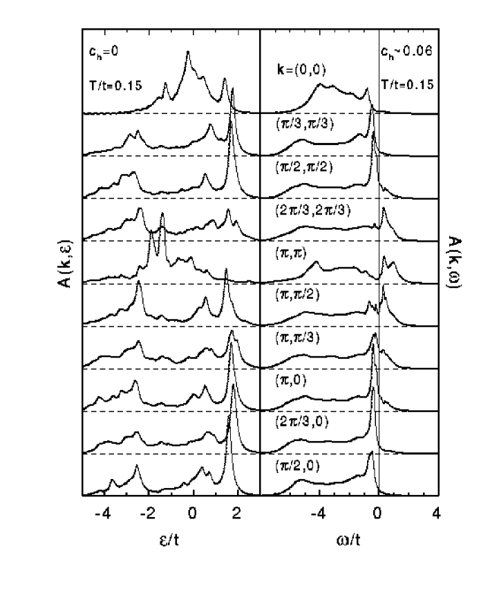
Figure 7.1: Spectral functions for the undoped AFM (left), and for a system with finite doping $c_{h}=1/N$ (right), both obtained on lattices with $N=16,18$ sites.

In Fig. 7.2 we present the $T$-dependence of the spectral function at $\vec{k}^{*}=(\pi/2,\pi/2)$, which corresponds to the g.s. momentum of a hole in an AFM. We realize from Fig. 7.2 that there is a significant spectral change going from $T\sim 0$ to $T>J$. Namely, in the high-$T$ regime the QP peak becomes progressively broader and merges with the incoherent background, which at the same time loses the detailed structure (resonance peaks). This development is plausible since for $T>J$ we are dealing essentially with the hole propagation in a random spin background well accounted for within the RPA (Brinkman and Rice 1970).

Figure 7.2: Spectral function $A(\vec{k}^{*},\varepsilon)$ for the undoped AFM at several $T$.

At $T<J$ the QP energy $E_{\vec{k}}$ and the corresponding weight $Z_{\vec{k}}~{}$, as determined by equations (7.10), show only a weak $T$ dependence and we get $\tilde{Z}=Z_{\vec{k}^{*}}(T)\sim 0.16$. We note that this value is obtained for the spectral function normalized according to the relation (7.5) with $\alpha=1/2$. It is easy to see that in order to make a comparison with the usual definition of the QP weight of an AFM polaron (Kane et al. 1989, Martinez and Horsch 1991) we should rather take ${\cal Z}=\tilde{Z}/\alpha$ and our value ${\cal Z}\sim 0.32$ is consistent with the one ${\cal Z}\sim 0.284$, obtained within the self-consistent Born approximation for $J/t=0.3$.

7.3 Spectral functions at finite doping

In Figs. 7.1, 7.3 we present the gradual development of spectral functions towards the optimum doping. For $c_{h}\sim 0.06$ and $c_{h}\sim 0.12$ results obtained on systems with $N=16,18$ sites are combined for $N_{h}=1$ and $N_{h}=2$ holes, respectively. As distinct to the undoped case, the spectra are broadened with Lorentzians of variable width according to $\delta=\delta_{0}+(\delta_{\infty}-\delta_{0})\tanh^{2}(\omega/\Delta)$, with $\delta_{\infty}=0.2t$, $\delta_{0}=0.04t$, and $\Delta=1.0t$. In this way sharper (well resolved) $\omega\sim 0$ features remain unaffected, while some of finite-size structures at higher $|\omega|>t$ are smoothened out. In any case, $\delta$ is always taken smaller than the energy widths of main spectral features.

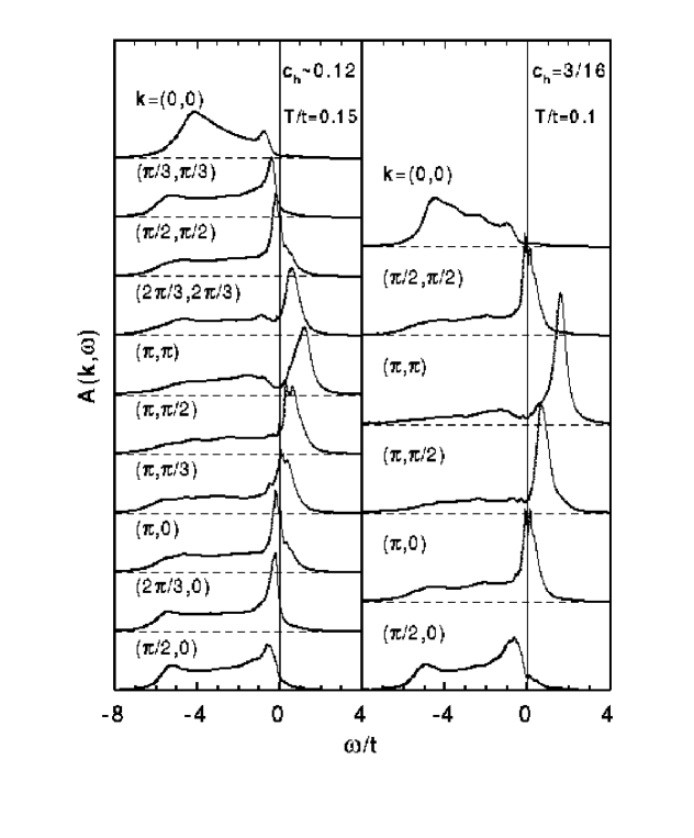
Figure 7.3: $A(\vec{k},\omega)$ for $N_{h}=2$ holes on $N=16,18$ sites, and for $N_{h}=3$ holes on $N=16$ sites.

At finite doping we observe in $A({\vec{k}},\omega)$ at all available $\vec{k}$ a coexistence of sharper features, associated with coherent QP peaks, with a broad incoherent background, as already established in ED studies (Stephan and Horsch 1991, Moreo et al. 1995). Coherent peaks disperse through $\omega=0$ as ${\vec{k}}$ crosses the FS. Within the given resolution in the ${\vec{k}}$ space the FS appears to be large for all $c_{h}\gtrsim 0.12$, consistent with the Luttinger theorem (Luttinger 1960). An analogous dispersion is observed for the underdoped case $c_{h}\sim 0.06$, although the latter one requires a more careful interpretation as given lateron. The total QP dispersion $W$ is broadening as $c_{h}$ is increasing, qualitatively consistent with the slave boson result where $W\propto c_{h}t+\chi J$ (Baskaran et al. 1987, Wang et al. 1991).

7.3.1 Intermediate doping

We first discuss in more detail the regime of intermediate doping (Jaklič and Prelovšek 1997), in our lattices $c_{h}\sim 0.12$ and $c_{h}=3/16\sim 0.19$. In Fig. 7.4 we show $\Sigma({\vec{k}},\omega)$ evaluated for $c_{h}=3/16$ at $T=0.1~{}t\sim T_{fs}$. We first notice an asymmetry between the PES ($\omega<0$) and the IPES ($\omega>0)$ spectra at all ${\vec{k}}$. $\Sigma^{\prime\prime}({\vec{k}},\omega)$ are small for $\omega>0$, as compared to $\omega<0$. For ${\vec{k}}$ outside the FS this implies a modest QP damping, consistent with sharp IPES peaks seen in $A({\vec{k}},\omega)$ in Fig. 7.3, containing the major part of the spectral weight. $\Sigma^{\prime}({\vec{k}},\omega)$ shows an analogous asymmetry, in the region $\omega>0$ resembling moderately renormalized QP. Due to the definition (7.7) the slope of $\Sigma^{\prime}$ is not zero even at $|\omega|\gg t$.

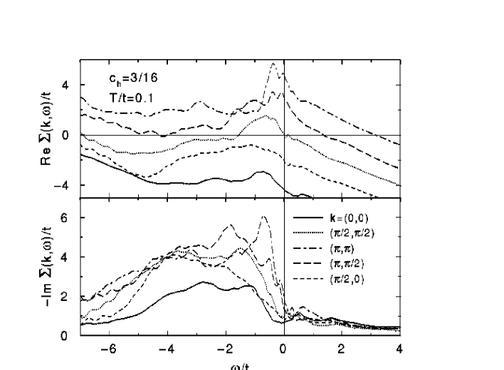
Figure 7.4: Self energy $\Sigma(\vec{k},\omega)$ for $c_{h}=3/16$ at various ${\vec{k}}$.

The behaviour on the PES ($\omega<0$) side is very different. For all ${\vec{k}}$, $-\Sigma^{\prime\prime}(\omega)$ are very large at $\omega<-t$, leading to overdamped QP structures. We should however distinguish two cases. For $\vec{k}$ well outside the FS, large $|\Sigma^{\prime\prime}(\omega<0)|>t$ does not invalidate a well defined QP at $\omega>0$, but rather induces a weak reflection (shadow) of the IPES peak at $\omega<0$, as well seen in Fig. 7.3 for ${\vec{k}}=(\pi,\pi)$. On the other hand, for ${\vec{k}}$ inside or near the FS the variation with $\omega$ is more regular, and can be directly related to the QP damping. Particularly remarkable feature in Fig. 7.4 is a linear $\omega$ dependence of $\Sigma^{\prime\prime}(\omega\lesssim 0)$ for ${\vec{k}}=(\pi/2,0)$ and ${\vec{k}}=(\pi/2,\pi/2)$. Meanwhile ${\vec{k}}=(0,0)$, being further away from the FS, seems to follow a different more LFL-type behaviour. Similar general conclusions follow also from results obtained for the lower doping $c_{h}=2/18$.

To address the latter point in more detail, we show in Fig. 7.5 the $T$ variation of $\Sigma^{\prime\prime}(\vec{k},\omega)$ for both dopings at selected ${\vec{k}}$ inside the FS. For $c_{h}=3/16$ the linearity of $\Sigma^{\prime\prime}(\omega)$ is seen in a broad range $-2t\lesssim\omega\lesssim 0$ at the lowest $T$ shown. Moreover, for this optimum doping the $T$ dependence is close to a linear one, taking into account a small residual (finite-size) damping $\eta_{0}>0$ at $\omega=0$. Data can be well described by

$$-\Sigma^{\prime\prime}(k\lesssim k_{F},\omega)=\eta_{0}+\gamma(|\omega|+\xi T),\qquad\gamma\sim 1.4,\quad\xi\sim 3.5.$$ (7.11)

Such a dependence is consistent with one of the proposed forms (2.4) within the MFL scenario, as well as with the conductivity relaxation $1/\tau(\omega)$ in the equation (5.17). In contrast, the $T$ dependence for $c_{h}=2/18$ seems somewhat different, and we find $-\Sigma^{\prime\prime}\propto\omega$ only in the interval $-t\lesssim\omega\lesssim-T$. This would indicate the consistency with the original MFL form (2.3) (Varma et al. 1989), however we should be aware that in the underdoped regime finite-size effects are larger at given $T$.

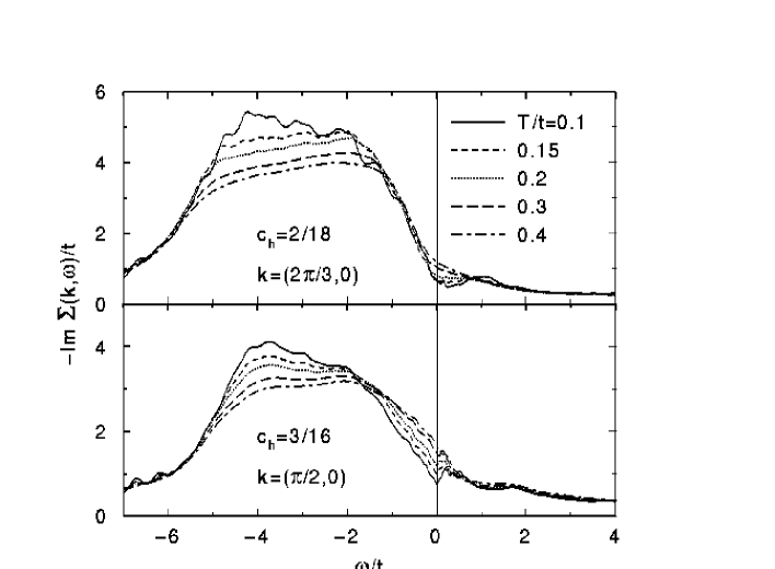
Figure 7.5: $\Sigma^{\prime\prime}({\vec{k}},\omega)$ for $c_{h}=2/18$ and $c_{h}=3/16$ at different $T$ and selected ${\vec{k}}$ inside the FS.

Here we should comment on the manifestation of the FS in small fermionic systems. At $T,\omega\sim 0$ we are dealing in the evaluation of the expression (7.3) with the transition between g.s. of systems with $N_{h}$ and $N_{h}^{\prime}=N_{h}\pm 1$ holes, respectively. Since these g.s. states have definite momenta ${\vec{k}}_{0}$, they induce sharp QP peaks for particular ${\vec{k}}={\vec{k}}^{\prime}_{0}-{\vec{k}}_{0}$ defining in this way for a small system the FS, apparently satisfying the Luttinger theorem. At the same time the corresponding QP damping vanishes, i.e. $\Sigma^{\prime\prime}({\vec{k}},\omega\sim 0)\sim 0$.

From $\Sigma({\vec{k}},\omega)$ we can calculate QP parameters, as defined in equations (7.10). Results for $c_{h}\sim 0.12$ and $c_{h}\sim 0.19$ are presented by Jaklič and Prelovšek (1997). We note that parameters are of a limited meaning for $\vec{k}$ well inside FS due to a large damping $\Gamma_{\vec{k}}$. Otherwise, $E_{\vec{k}}$ shows the enhancement of the dispersion with $c_{h}$, while $\Gamma_{\vec{k}}<E_{\vec{k}}$ for $|{\vec{k}}|>k_{F}$. To establish the relation with the FL theory one has to evaluate QP parameters at the FS ${\vec{k}}\sim{\vec{k}}_{F}$. Of particular importance is the renormalization factor $\tilde{Z}=Z_{{\vec{k}}_{F}}(T=0)$. We find that at lowest $T\sim T_{fs}$ $Z_{\vec{k}_{F}}(T)$ is still decreasing as $T$ is lowered, e.g. a variation (cca. 20%) is found within the interval $0.1<T/t<0.3$. This is not inconsistent with the MFL form $\tilde{Z}^{-1}\sim\ln(\omega_{c}/T)$, although such a conclusion should be taken with care due to narrow $T$ interval.

Regarding the size of $\tilde{Z}$ at low but finite $T>0$ we note, that the value of the momentum distribution function is very close to the maximum (7.6) for all $k<k_{F}$, i.e. $\bar{n}_{\vec{k}}\sim(1+c_{h})/2$ (Stephan and Horsch 1991). Taking the FS volume according to the Luttinger theorem $V_{FS}/V_{BZ}=(1-c_{h})/2$ and assuming that $\bar{n}_{\vec{k}}$ falls monotonously with $k$, this implies an inequality for the discontinuity $\tilde{Z}$,

$$\tilde{Z}=\delta\bar{n}_{\vec{k}_{F}}<{2c_{h}\over 1+c_{h}}.$$ (7.12)

One should keep in mind that a discontinuity is meaningful at $T\sim 0$, while at $T>0$ it indicates only a gradual step. Still we find a consistent result $\tilde{Z}=0.28$ for $c_{h}=3/16$, while for $c_{h}=2/18$ the value $\tilde{Z}=0.35$ is somewhat larger, possibly due to higher $T$ used in calculations.

An analogous argument can be used to explain the electron-hole asymmetry of $A(\vec{k},\omega)$. Holes added to the system at $k<k_{F},\omega<0$ move in an extremely correlated system, strongly coupled to the spin dynamics (Prelovšek 1997a), the latter also exhibiting the anomalous MFL-type behaviour, as given by the expression (6.13). On the other hand, states for $k>k_{F}$ are not fully populated, allowing for a moderately damped motion of added electrons with $\omega>0$.

Let us comment here on the relevance of our results to ARPES spectra near the optimum doping. The main observation is that for $k<k_{F}$ we find the linewidth typically $\Gamma\sim t\sim 0.4~{}{\rm eV}$ well compatible with experiments at ${\vec{k}}$ away from the FS and at intermediate doping (Shen and Dessau 1995, Ding et al. 1996, Marshall et al. 1996). Also the MFL form has been claimed to describe better the experiments (Olson et al. 1990), although this point is still controversial (see Shen and Dessau 1995).

7.3.2 Overdoped and underdoped regime

Let us turn from the intermediate doping first to the overdoped regime. Spectra at higher doping $c_{h}=4/16$ and $c_{h}=5/16$ are shown in Fig. 7.6. While $A({\vec{k}},\omega)$ at $c_{h}=4/16$ are still qualitatively similar to the spectra at intermediate doping, at $c_{h}=5/16$ they are already showing a substantially different behaviour. In the latter case the incoherent background in the PES spectrum is reduced while QP peaks for $k<k_{F}$ are sharpened and all of them are essentially underdamped with $\Gamma_{\vec{k}}<E_{\vec{k}}$. Nevertheless, we still have $\Gamma_{\vec{k}}\sim E_{\vec{k}}$ so it is not evident whether this is already a (more) normal LFL.

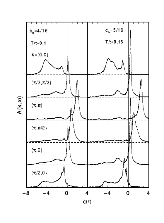
Figure 7.6: $A(\vec{k},\omega)$ for $c_{h}=4/16$ and $c_{h}=5/16$.

The proper analysis of the underdoped regime is even more delicate. At $c_{h}\sim 0.06-0.12$, as presented in Figs. 7.1, 7.3, a ’shadow’ feature is clearly seen in $A({\vec{k}},\omega)$ for $k>k_{F}$. Namely, along with the principal peak at $\omega>0$ a weak bump in the $\omega<0$ part of the spectrum appears. In $\Sigma^{\prime}(\vec{k},\omega)$ for $k>k_{F}$ this effect emerges as a strong oscillation, most pronounced for ${\vec{k}}=(\pi,\pi)$. It leads even to a double solution of the equation (7.10) for $E_{\vec{k}}~{}$, analogous to the phenomena within the spin-bag scenario (Kampf and Schrieffer 1990). This effect is becoming less visible at larger doping, e.g. at $c_{h}=3/16$, so its disappearance is related to the reduction of the AFM correlation length $\xi\sim 1$.

Let us try to make the contact with recent ARPES measurements on underdoped BISCCO (Marshall et al. 1996), which show the opening of the pseudogap even for $T>T_{c}$, in particular near the $\vec{k}^{**}=(\pi,0)$ point, where the FS seems to disappear. On the other hand the QP peak disperses through the FS along the $\Gamma$-M direction where the FS seems to be well defined. If we look closer at Fig. 7.1 for the lowest finite doping $c_{h}\sim 0.06$, we can recognize very similar features. We realize that close to $\vec{k}^{**}$, the PES part shows spectra very analogous to the undoped AFM in Fig. 7.1, where due to the doubling of the Brillouin zone the dispersion is expected to reach maximum at $\vec{k}^{*}=(\pi/2,\pi/2)$ (note however that on a $4\times 4$ lattice with n.n. hopping $k^{*}$ and $k^{**}$ are equivalent) and folds back for $\vec{k}$ outside the reduced AFM zone. E.g., in Fig. 7.1 for $c_{h}\sim 0.06$ we can clearly recognize PES peaks also for $\vec{k}=(\pi,\pi/3)$ and $\vec{k}=(\pi,\pi/2)$, being lower in $\omega$ than the QP peak at $\vec{k}^{*}$. Such a dispersion is also seen in ARPES. At the same time there is for both mentioned $k>k^{*}$ also a visible peak in the IPES part, which can be interpreted as a QP dispersing through the FS. The PES and the IPES peak in this case are separated by a gap, which does not seem to be a finite-size effect, and is qualitatively consistent with the ARPES feature (Marshall et al. 1996). It should be also noted that along the $\Gamma$-M direction the QP dispersion is closer to a normal metallic one with much less pronounced ’shadows’ for $k>k_{F}$.

7.3.3 Influence of next-nearest-neighbour hopping

It is evident from spectral functions at the intermediate doping, e.g. in Figs. 7.3, 7.6 that the shape of the FS obtained within the $t$-$J$ model is closer to a circular one than to the one found in cuprates via ARPES experiments (Shen and Dessau 1995), where e.g. $\vec{k}^{**}$ is inside the FS. It has been well established that such a FS topology can be reproduced by adding the n.n.n. hopping term (2.7) with $t^{\prime}<0$ (Tohyama and Maekawa 1994). It is however still an open question whether the modified hopping and different FS topology are essential for the anomalous properties of cuprates.

In order to see the qualitative changes introduced by the n.n.n. hopping, we present in Fig. 7.7 $A(\vec{k},\omega)$ at fixed doping $c_{h}=3/16$ for two different $t^{\prime}/t=-0.2$ and $t^{\prime}/t=-0.35$. It is evident that $t^{\prime}<0$ lifts the degeneracy between of the $\vec{k}^{*}$ and $\vec{k}^{**}$ even in the $4\times 4$ lattice. Also the QP dispersion changes and the QP peak with $\vec{k}^{*}$ is now at $\omega>0$, i.e. outside the FS, while the QP with $\vec{k}^{**}$ moves inside the FS. The effect is enhanced for larger $|t^{\prime}/t|$. It is however important to realize that other QP properties are not essentially changed, in particular we find that the self energy $\Sigma^{\prime\prime}(\vec{k},\omega)$ remains qualitatively similar to the case with $t^{\prime}=0$.

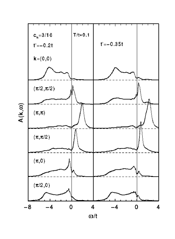
Figure 7.7: $A(\vec{k},\omega)$ for $c_{h}=3/16$ with nonzero n.n.n. hopping: $t^{\prime}/t=-0.2$ and $t^{\prime}/t=-0.35$.

7.4 Density of states

Finally we present in Fig. 7.8 the doping dependence of the single-particle DOS ${\cal N}(\varepsilon)$ (Jaklič and Prelovšek 1997), as defined in the equation (7.8). In a weakly doped system with $c_{h}\sim 0.06$, a QP coherent peak (of width $\sim 2J$) is seen at $\omega=\varepsilon-\mu\lesssim 0$. Besides that, a broad background due to well understood incoherent hole motion is dominating $\omega\ll 0$. At such low doping the electron $\omega>0$ part of the DOS is weak, with the total intensity $2c_{h}$ as compared to $1-c_{h}$ of the hole part. With increasing $c_{h}$ the hole incoherent background does not reduce appreciably in intensity, while the coherent dispersion near the Fermi energy widens and cannot be well distinguished in ${\cal N}(\varepsilon)$ from the background. At the same time, the electron part of the DOS is increasing, both in the weight and in the width. Note that oscillations which appear for $\omega>0$ at higher doping $c_{h}>3/16$ are essentially finite-size effects. Namely we are dealing with a restricted number of finite-size $\vec{k}$ while QP peaks are becoming quite narrow. Such effects are even more pronounced in overdoped systems with $c_{h}>0.25$, where the incoherent part is finally losing its intensity and the coherent QP are dominating the whole $\varepsilon$ regime. It should be also mentioned that the introduction of the n.n.n. hopping $t^{\prime}\neq 0$, in spite of a significant change of the FS shape, does not seem to induce an essential change within the DOS.

Figure 7.8: Single-particle DOS ${\cal N(\varepsilon)}$ for different dopings at fixed $T/t=0.15$. For $c_{h}\sim 0.06$ and $c_{h}\sim 0.12$ we present joined DOS for $N=16,18$ systems with $N_{h}=1$ and $N_{h}=2$, respectively. The thin vertical lines denote the chemical potential $\mu(T)$.

Let us comment here the relation with the entropy $s$, Fig. 4.3a. If we assume the low-$T$ form as follows from the LFL theory (Abrikosov et al. 1965), we get

$$s={\pi^{2}{\cal N}(\mu)\over 3\tilde{Z}}~{}T.$$ (7.13)

We see from Fig. 7.8 that ${\cal N}(\mu)$ is only weakly doping dependent at intermediate $c_{h}$ and actually also quite close to the free-fermion value (assuming a tight-binding model with the hopping parameter $t$). Taking $\tilde{Z}\sim 0.28$ for $c_{h}=3/16$, we get $s\sim 0.29~{}k_{B}$ at $T=0.1~{}t$, quite consistent with thermodynamic results in Sec. 4.2. Here the surprising fact is that such $s$ represents a large increase over the undoped AFM and appears due to a very low concentration of mobile holes introduced into an AFM.

Let us now look closer on ${\cal N}(\varepsilon)$ in the underdoped regime. We realize quite clearly that at $c_{h}=0.12$ a pseudogap starts to appear in the DOS at $\omega=\varepsilon-\mu\sim 0$ and becomes even more pronounced at $c_{h}\sim 0.06$. It is evidently related to a similar phenomenon in $A(\vec{k},\omega)$ in Fig. 7.1. In order to establish the origin of such a gap, we follow in Fig. 7.9 the variation of ${\cal N}(\varepsilon)$ with $T$. We find that the gap structure disappears at $T>J$, so it must be related to the onset of the short-range AFM order. Also the gap energy $\Delta\epsilon\lesssim t$ seems to be determined rather by $J$. It is plausible that the onset temperature is related to pseudogap scale $T^{*}$, discussed before in relation with the maximum in $\chi_{0}(T)$, and with the crossover in $\rho(T)$.

 

Figure 7.9: ${\cal N(\varepsilon)}$ at various $T$ for dopings: (a) $c_{h}=1/20$ and (b) $c_{h}=2/18$.

Recently the DOS has been measured via the integrated PES and IPES for LSCO compound in a wide range of doping $0<c_{h}<0.3$ (Ino et al. 1997b). More reliable are PES spectra proportional to ${\cal N}^{+}(\omega)={\cal N}(\omega+\mu)f(\omega)$, giving information on the hole part $\omega<0$. Some features are well consistent with our results. In the overdoped regime $c_{h}>0.2$ ${\cal N}^{+}(\omega<0)$ appears quite flat. At the same time, there is a substantial and broad IPES contribution indicating an enhanced DOS at $\omega>0$. On the other hand, for $c_{h}<0.17$ a pseudogap starts to emerge gradually at $\omega\lesssim 0$. E.g., the inflection point in ${\cal N}^{+}(\omega)$ moves from $\omega\sim 0$ toward $\omega\sim-0.2~{}$eV at lowest dopings. This is quite close to values found in Figs. 7.9. Thus the gap scale indeed seems to be related to the pseudogap scale $T^{*}$ discussed in connection with $\chi_{0}$. Note that the latter is substantially larger than the leading-edge shift $\sim 30$ meV found in ARPES (Marshall et al. 1996). Still it is well possible that both phenomena are closely related.

8 Other properties

8.1 Electron density correlations

It is interesting to study also electron-density dynamics, as contained within the dynamical charge susceptibility $\chi_{c}(\vec{q},\omega)$ and the corresponding density correlation function $N(\vec{q},\omega)$, defined by

$$\chi_{c}^{\prime\prime}(\vec{q},\omega) = e_{0}^{2}(1-e^{-\beta\omega})N(\vec{q},\omega),$$

$$N(\vec{q},\omega) = {\rm Re}\int_{0}^{\infty}dt\;e^{i\omega t}\langle n_{\vec{q}}(t)n_{-\vec{q}}(0)\rangle,$$ (8.1)

$$n_{\vec{q}} = (1/\sqrt{N})\sum_{i}e^{i\vec{q}\cdot\vec{R}_{i}}n_{i}.$$

Recently several numerical and analytical studies within the $t$-$J$ model have been devoted to static $N(\vec{q})$ (Putikka et al. 1994) as well as to dynamical $N(\vec{q},\omega)$ (Tohyama et al. 1995, Eder et al. 1995, Khaliullin and Horsch 1996) at $T=0$, mainly in connection with the interesting conjecture of the charge-spin separation (Anderson 1987, Baskaran et al. 1987) in layered cuprates. A parallel study of charge correlations $N(\vec{q},\omega)$ and the spin structure factor $S(\vec{q},\omega)$ however reveals quite an essential difference between an 1D Luttinger liquid and a 2D doped AFM (Tohyama et al. 1995), as well as between charge and spin fluctuations. Typically, $N(\vec{q},\omega)$ show a broad peak at high $\omega\sim 6~{}t$ at $\vec{q}\sim\vec{Q}$ due to the incoherent motion of holes, while at $q\to 0$ density fluctuations narrow in a collective acoustic-like mode (Khaliullin and Horsch 1996). In contrast to $S(\vec{q},\omega)$, $N(\vec{q},\omega)$ spectra seem to scale linearly with $c_{h}$ at low doping (Eder et al. 1995). It should be also noted that quite generally $N(q\to 0,\omega)$ fluctuations can be related to (anomalous) current correlations $C(\omega)$ through the particle-number conservation, so an anomalous behaviour is quite possible for $N(\vec{q},\omega)$ as well.

The investigation of $N(\vec{q},\omega)$ at $T>0$ has not been performed so far. We present here some results, using the FTLM in analogy with the evaluation of $S(\vec{q},\omega)$ in Sec. 6. Our aim is again twofold. On one hand, FTLM gives smoother spectra at $T>T_{fs}$, which could be compared to g.s. ED results. More interesting is the low-frequency regime $\omega<J$, which cannot be studied reliably in g.s. calculations, and moreover the $T$ dependence of spectra in this regime.

In Fig. 8.1 we present normalized spectra $N(\vec{q},\omega)/c_{h}$ for nonequivalent $\vec{q}$ on a lattice of $N=18$ sites and fixed $T=0.2~{}t$. In this case we use $J/t=0.4$. Shown are results for $c_{h}=1/18$ and $c_{h}=3/18$, belonging to regimes of low doping and optimum doping, respectively. We notice that normalized spectra are very similar for both $c_{h}$, at least for larger $q$, taking into account also that a more detailed structure for $c_{h}=1/18$ is partly due to finite size effects. Our results are in general close to previous numerical (Tohyama et al. 1995, Eder et al. 1995) and analytical (Khaliullin and Horsch 1996) results. It is characteristic that at $\vec{q}\sim\vec{Q}$ the intensity is nearly exhausted by a large peak at $\omega\sim 6t$. As expected from conservation laws spectra are narrowing for $q\to 0$.

Figure 8.1: Normalized density correlation spectra $N(\vec{q},\omega)/c_{h}$ at fixed $T/t=0.2$ and $J/t=0.4$ at two dopings: $c_{h}=1/18$ and $c_{h}=3/18$.

It is however remarkable that in spite of quite low $T$ in Fig. 8.1 $N(\vec{q},\omega\to 0)$ does not seem to approach zero for any $\vec{q}$, the effect being more visible for smaller $q$. We follow the evolution of density fluctuations with $T$ at intermediate doping $c_{h}=3/16$ for chosen $\vec{q}=(\pi/3,\pi/3)$ in Fig. 8.2. It is evident that $N(\vec{q},\omega)$ is nearly $T$ independent even for $\omega<T$. The behaviour is quite similar to the one observed for local spin correlations $\bar{S}(\omega)$ in Fig. 6.5 and is consistent with the MFL assumption (2.2) for the charge susceptibility $\chi_{c}^{\prime\prime}(\omega)$, requiring via the equation (8.1) $N(\vec{q},\omega\to 0)=const$ independent of $T$. The MFL behaviour of $N(\vec{q},\omega)$ at intermediate doping is not entirely surprising due to the connection to the anomalous MFL-type $C(\omega)$ and optical conductivity $\sigma(\omega)$, as well due to the relation of the electron dynamics to anomalous spin fluctuations $S(\vec{q},\omega)$ (Prelovšek 1997a).

Figure 8.2: $N(\vec{q},\omega)$ for $\vec{q}=(\pi/3,\pi/3)$ and different $T$ at fixed $c_{h}=3/18$.

$N(\vec{q},\omega)$ have been mainly the subject of theoretical considerations so far. It should be however noted that a relation could be established with experimentally relevant dielectric function $\epsilon(\vec{q},\omega)$, if the model would incorporate also the long-range Coulomb repulsion between electrons. Such an additional interaction could be possibly treated within a framework of an random-phase-like analysis. It would be desirable since $\epsilon(\vec{q},\omega)$ can be measured also in cuprates via the electron-energy loss spectroscopy (Nücker et al 1989) which yields directly Im$[1/\epsilon(\vec{q},\omega)]$.

8.2 Electronic Raman response

One of very useful probes for the investigation of excitations in an AFM has been the Raman scattering. Using the latter method, it has been also established that the reference insulating cuprates correspond well to a planar Heisenberg AFM, where pronounced Raman resonance processes at low $T$ are attributed to two-magnon excitations (Lyons et al. 1988, Singh et al. 1989).

A general framework for the theoretical explanation of Raman processes in correlated systems has been so far given within the Hubbard model, where the effective Raman operator for resonant and off-resonant conditions has been derived (Shastry and Shraiman 1990). Still there are several unresolved questions concerning Raman processes in cuprates, and more generally in doped AFM. One puzzling aspect concerns the observed pronounced $T$ dependence of the two-magnon peak in undoped cuprates (Knoll et al. 1990). The latter has been interpreted as the phonon-induced broadening, but also invoking higher-order resonant processes (Chubukov and Frenkel 1995). Another problem is the doping dependence of Raman spectra. Recent experiments, performed on YBCO materials in the resonant regime (Blumberg et al. 1994), show a dramatic increase of the broadening of the two-magnon peak with doping, so that spectra appear essentially flat in the normal phase when approaching the optimum doping. At the same time, the peak position does not move appreciably.

Here we consider only the resonant Raman processes, since most experiments are performed in the resonant regime. In contrast to response functions considered in previous sections, the operator relevant for the resonant Raman scattering cannot be determined uniquely within the $t$-$J$ model, since it necessarily involves higher (resonant) levels. Still we can adopt a view that more complete (e.g. three-band) model for cuprates can be mapped onto an effective Hubbard model (Hybertsen et al. 1990) for resonant transitions of interest. Within the Hubbard model near half-filling the Raman-scattering operator has been derived in the limit $~{}t/U\ll 1$ (Shastry and Shraiman 1990) yielding the well known form for the Heisenberg AFM (Parkinson 1969),

$$R=A\sum_{\langle ij\rangle}(\vec{\epsilon}_{inc}\cdot\vec{r}_{ij})(\vec{\epsilon}_{sc}\cdot\vec{r}_{ij})(\vec{S}_{i}\cdot\vec{S}_{j}-{1\over 4}n_{i}n_{j}),$$ (8.2)

where $\vec{\epsilon}_{inc},\vec{\epsilon}_{sc}$ are the incident and the scattered electric-field unit vectors, respectively, and the amplitude factor $A=4t^{2}/(U-\omega_{inc})\propto J$ incorporates the resonance at the incident-light frequency $\omega_{inc}\sim U$. The Raman spectral function is then given by

$$I(\omega)={1\over\pi N}{\rm Re}\int_{0}^{\infty}dt~{}e^{i\omega t}\langle R(t)R(0)\rangle,$$ (8.3)

which can be calculated at $T>0$ using the FTLM analogous to other correlation functions.

Within the $t$-$J$ model with finite doping the Raman intensity $I(\omega)$, corresponding to the operator (8.2), has been evaluated so far at $T=0$ using the ED (Dagotto and Poilblanc 1990), while for the undoped AFM also $T>0$ has been studied using the full diagonalization (Bacci and Gagliano 1991). Results obtained via the FTLM have an advantage over previous ones also for low $T$, since the Raman intensity is not expected to be singular for $T\to 0$, so much smoother spectra are obtained by using small but finite $T>T_{fs}$.

We restrict our analysis to the dominant $B_{1g}$ scattering geometry with $\vec{\epsilon}_{inc}=(\vec{e}_{x}+\vec{e}_{y})/\sqrt{2}$ and $\vec{\epsilon}_{sc}=(\vec{e}_{x}-\vec{e}_{y})/\sqrt{2}$. The undoped AFM at $T>T_{fs}\sim J/2$ has been studied by Prelovšek and Jaklič (1996), and reveals at low $T$ a two-magnon Raman peak at $\omega\sim 3.3~{}J$, consistent with experiments. The width is however quite narrow and starts to broaden substantially only at higher $T\sim J$, where a gradual transition to a broad featureless spectrum occurs. Hence other mechanisms have to be invoked to account for the observed pronounced $T$-dependent width at lower $T\ll J$ (Knoll et al. 1990).

In doped systems $T$ plays a less essential role and typically we observe only a weak decrease of the Raman intensity in the interval $T/J=0.3-1.0$ (Prelovšek and Jaklič 1996). On the other hand, the dependence on doping is essential, as evident from Fig. 8.3, where we present $I(\omega)$ for various dopings $c_{h}\leq 0.25$ at lowest $T=0.15~{}t>T_{fs}$. Already the smallest nonzero doping $c_{h}=0.05$ increases dramatically the width of the two-magnon peak, while spectral features become overdamped on approaching the optimum doping $c_{h}\sim 0.15$. It is however remarkable, that the peak position does not shift appreciably in the underdoped regime $c_{h}\leq 0.1$. Only for $c_{h}>0.15$ the spectra change to a broad central-peak form with a maximum at $\omega=0$.

Figure 8.3: Raman intensity $I(\omega)$ for different dopings $c_{h}$ at fixed $T=0.15~{}t$.

How can we interpret the above results for the $B_{1g}$ resonant Raman scattering ? Up to the overdoped situation $c_{h}\sim 0.3$ the scattering seems to be dominated by the spin-exchange part (8.2), since the latter determines the low-energy fluctuations even at the optimum doping. Still, there are evident changes with doping, since the reduced AFM correlation length at larger $c_{h}$ induces a large broadening of the Raman two-magnon peak and a reduction of its intensity. In this respect the doped system behaves quite similarly to an undoped AFM but at elevated $T\sim J$.

A systematic resonant-Raman scattering study has been recently performed on a sequence of YBCO materials (Blumberg et al. 1994). It seems that in the underdoped regime our model results well reproduce experimental ones, both regarding the shape of the Raman spectra and their intensity variation with doping. At optimum doping experiments still reveal a weakly pronounced peak at the same frequency $\omega\sim 3~{}J$, while our results on Fig. 8.3 already reveal a maximum at $\omega=0$, nevertheless both spectra are nearly flat.

8.3 Thermoelectric power

Among other transport properties the thermoelectric power (TEP) or the Seebeck coefficient $S$ is one of the most frequently investigated. Within the cuprate family TEP has been measured for several materials, for an overview see e.g. Kaiser and Uher (1991) and more recent analyses (Tallon et al. 1995, Cooper and Loram 1996). Again an universal behaviour has emerged depending mainly on hole doping. For weakly doped materials $S$ is large and positive, with some $T$ dependence at higher $T$. With increasing doping TEP $S$ decreases rapidly. It also falls off nearly linearly with $T$, but with a rather small slope. Quite consistently $S$ is nearly vanishing for the optimum doping and changes sign to a negative one in overdoped materials. This variation has clearly some parallel with the doping dependence of the Hall coefficient $R_{H}$, also showing a transition from a hole-like behaviour $R_{H}>0$ at low doping into an electron-like $R_{H}<0$ in overdoped samples. It seems plausible that both anomalous properties are related and emerge from strong correlations in these materials.

Theoretically TEP in doped AFM or more generally in strongly correlated metals has not attracted much attention so far (Hildebrand et al. 1997). This is not surprising, since it seems to require the understanding of both electrical and thermal currents.

Within the linear response theory (Mahan 1990) the TEP can be expressed in terms of particle current $j$ and energy current $j_{E}$ correlation functions,

$$S={1\over e_{0}T}\left[\mu-{C_{j_{E}j}(\omega\to 0)\over C(\omega\to 0)}\right],$$ (8.4)

where mixed correlation function $C_{j_{E}j}(\omega)$ is defined in analogy with the expression (5.1) for $C(\omega)$.

The evaluation of $S(T)$ thus requires the calculation of $C_{j_{E}j}(\omega)$, in addition to the current-current correlation function $C(\omega)$ discussed extensively in Sec. 5. It is straightforward to derive the expression for $j_{E}$, nevertheless the operator is more involved due to three-site terms. We do not intend to give here a more complete analysis of $C_{j_{E}j}(\omega)$ which will be presented elsewhere. We mention however only a preliminary observation, that $C_{j_{E}j}(\omega)$ and $C(\omega)$ appear to be closely related,

$$C_{j_{E}j}(\omega)=\zeta C(\omega),$$ (8.5)

i.e. $\zeta$ is nearly $\omega$ independent for $\omega<t$, but as well $T$ independent at low $T<J$. Since we are dealing at $c_{h}>0$ with a metal, although with a strange one, we expect a finite $|S(T\to 0)|<\infty$. Hence we deduce from the equation (8.4) the condition $\zeta=\mu(T=0)$. Our numerical results for $\zeta$ are indeed consistent with this assumption.

We thus arrive at the simplified expression,

$$S\sim{1\over e_{0}T}[\mu_{h}(T=0)-\mu_{h}(T)],$$ (8.6)

which involves only $\mu_{h}(T)$, studied in Sec. 4.1 and shown in Fig. 4.1. In the low-$T$ regime of interest we claim in a broad regime of doping $c_{h}<0.3$ a linear variation (4.3) of $\mu_{h}(T)$. This leads directly to $S\sim-\alpha S_{0}$ where $S_{0}k_{B}/e_{0}=86\mu V/K$. It is evident from Fig. 7.3 that $\alpha$ is changing sign from a negative for $c_{h}<c_{h}^{*}$ to a positive one for $c_{h}>c_{h}^{*}$. In Fig. 8.4 we plot our result for $S(c_{h})$. Note that due to simplifications involved in the expression (8.6) we do not intend to consider the $T$ variation, hence our results apply to lowest reachable $T\lesssim T_{fs}\sim 0.1~{}t$. For comparison we present on the same plot also experimental results for LSCO and oxygen deficient YBCO, taken from Cooper and Loram (1996), whereby data refer to the normal state at $T\sim 300K$. Qualitative agreement between theory and experiment is quite reasonable. In LSCO values of $S$ are decreasing with doping, while $S$ is quite high at low doping $c_{h}<0.05$. Towards optimum doping $S$ essentially vanishes. Similar is the trend for YBCO data, although there are clearly quantitative differences. The main disagreement between the calculated and experimental $S$ is in the overdoped regime, where our results indicate $S<0$ with probably too large values. It is however well possible that in this regime our analysis is not adequate, first due to $\mu_{h}(T)$ approaching more normal LFL $T^{2}$ dependence, as well as due to the breakdown of the relation (8.5).

Figure 8.4: Thermoelectric power $S$ vs. $c_{h}$ for $T/t=0.1$. Experimental result for LSCO and oxygen deficient YBCO are taken from Cooper and Loram (1996).

9 Discussion

In the absence of accepted microscopic or phenomenological theories, which would at least qualitatively describe normal-state properties of cuprates in the whole doping regime, it is also hard to summarize our numerical results in a compact manner.

It is first important to understand which phenomena determine the optimum doping in cuprates and in microscopic models. In cuprates the optimum is defined by $T_{c}(c_{h}^{opt})=max$, but at least very close in doping, i.e., $c^{*}_{h}\sim c_{h}^{opt}$ are also materials where the low-$T$ electronic entropy $s$ and the uniform susceptibility $\chi_{0}$ are maximum (Loram et al. 1996), where the pseudogap scale disappears, i.e. $T^{*}\to T_{c}$ (Batlogg 1997), etc.

Within the $t$-$J$ model we can associate the optimum so far only with respect to normal-state properties, e.g. with $s(c_{h}^{*})=max$. Such a maximum has to exist at a nontrivial $c_{h}^{*}>0$ due to the relation (4.6) with $\mu_{h}(T)$, where the latter must change the sign from a weakly doped AFM (semiconductor-like regime) at $c_{h}\gtrsim 0$ to a regime of nearly free 2D fermions at $c_{e}\sim 0$. It is plausible that within the prototype model (2.6) $c_{h}^{*}$ is determined by the interplay of the spin exchange energy $E_{J}=\langle H_{J}\rangle$ and the (hole) kinetic energy $E_{t}=\langle H_{t}\rangle$. Since at low doping we get $|E_{t}|\propto tc_{h}$ and $|E_{J}|\propto J$ we can get a rough estimate $c_{h}^{*}\propto J/t\ll 1$. From such an argument it seems plausible that at $c_{h}\sim c_{h}^{*}$ the AFM correlation length becomes very short $\xi\sim 1$, while AFM correlations are essentially irrelevant in the overdoped regime $c_{h}>c_{h}^{*}$.

9.1 Universality at intermediate doping

It is evident from our results that normal-state properties are universal at the optimum doping $c_{h}\sim c_{h}^{*}$. Since the maximum $s(c_{h})$ is broad within the $t$-$J$ model also this regime is quite extensive, i.e. $0.15<c_{h}<0.25$ for chosen $J/t=0.3$. The main feature of this regime obtained in our study is the MFL-type dynamics in several response functions: the local spin susceptibility $\chi_{L}^{\prime\prime}(\omega)$, the optical conductivity $\sigma(\omega)$, density correlations $N(\vec{q},\omega)$, and spectral functions $A(\vec{k},\omega)$. It is characteristic that the dynamics in the low-$\omega$ ($\omega<J$) regime seems to be universal, i.e. it is determined solely by $T$ itself without any additional parameters, as concluded from equations (5.13) for $\sigma(\omega)$ and (6.13) for $\chi_{L}^{\prime\prime}(\omega)$. It should be however reminded that this universality could be restricted to a certain $T$ range, e.g. we can show its validity only for $T_{fs}<T<J$.

It seems that the origin of the universality is in the large degeneracy of the spin subsystem, where the frustration in induced by the hole doping. A plausible argument is that holes tend to induce FM correlations to minimize kinetic energy, while spins prefer an AFM ordering. In any case, only spins have enough degrees of freedom to explain large entropy $s\sim 0.4~{}k_{B}$ even at $T<J$.

Let us attempt an explanation for the universality of $\bar{S}(\omega)$ at $c_{h}\sim c_{h}^{*}$. From the explicit representation in terms of eigenstates,

$$\bar{S}(\omega)=(1+e^{-\beta\omega})\sum_{n,m}{e^{-\beta E_{n}}\over Z}|\langle\Psi_{n}|S_{i}^{z}|\Psi_{m}\rangle|^{2}\delta(\omega-E_{m}+E_{n}),$$ (9.1)

we can first discuss conditions that the response is $T$ independent for $\omega>T$. Since in this case the prefactor is constant, a naive requirement appears to be that low lying states $E_{n}-E_{0}<T$ have similar matrix elements to excited states with $E_{m}-E_{n}>T$. Nevertheless the validity of this observation clearly depends on the character and on the density of low-lying many-body states, and e.g. does not apply at low $T$ to a system with a unique g.s. As realized from the entropy results in Sec. 4.2 the degeneracy and the density of many-body states is clearly very large at the intermediate doping. To explain the $T$ independence of $\bar{S}(\omega)$ even for $\omega<T$, we recall the sum rule (6.11) and assume that there is no characteristic scale $\omega_{c}<T$ which could introduce an additional low-$\omega$ structure in $\bar{S}(\omega)$. A natural candidate for such a scale in an AFM is the (gap) frequency $\omega_{c}\sim c/\xi$ where $c$ is the spin wave velocity and $\xi$ the AFM correlation length. Here originates the essential difference between an undoped and the optimally doped AFM. In a pure AFM within the renormalized classical regime $\xi$ is exponentially large for $T\ll J$ (Chakravarty et al. 1989) and consequently $\omega_{c}\ll T$. On the other hand, at the intermediate doping $\xi$ appears to be short and not strongly $T$ dependent, i.e. $\xi\propto 1/\sqrt{c_{h}}$. The latter situation excludes $\omega_{c}<T<J$, hence leading to an universal $\bar{S}(\omega)$.

Turning to the discussion of $\sigma(\omega)$, as given by the equation (5.13), we realize that it is not meaningful to associate $1/\tau(0)\propto T$ with a current relaxation rate. Namely the current-current correlation function $C(\omega)$ shows a broad uniform spectrum indicating on a very fast current decay with $1/\tilde{\tau}\sim 2t$. Thus it seems that a general condition for the validity of the specific MFL form (5.13) is a fast current decay with $1/\tilde{\tau}\gg T$. This could happen due to holes moving in a disordered spin subsystem, which leads to entirely incoherent collisions among holes and the appropriate mean free path $l_{s}$ is only few unit cells. Hence it seems that we are dealing with a novel phenomenon of quantum diffusion which follows an universal form (5.13).

In an analogous way also the relaxation of single electron states near FS is affected, as manifested in the MFL form of the self energy $\Sigma(\vec{k},\omega)$, equation (7.11). Anyhow it is plausible that the QP damping $\Sigma^{\prime\prime}(k\sim k_{F},\omega)$ and the current relaxation $1/\tau(\omega)$, as given by the equation (5.17), are closely related. There are also phenomenological arguments (Littlewood and Varma 1991) which indicate that the MFL-type dynamics of a boson (spin) subsystem implies a MFL behaviour of the electron propagator. Recently such a relation has been derived by one of the authors (Prelovšek 1997a), employing a decoupling approximation for the projected $G^{R}(\vec{k},\omega)$.

On the other hand it should be stressed that within the same regime certain electronic properties appear quite normal, i.e. close to the LFL behaviour. First, spectral functions indicate on a rather well defined large FS following the Luttinger theorem. This seems to indicate that correlated electronic state evolves continuously from a noninteracting one, whereby the FS can be traced to momenta of lowest (g.s.) many-body states. It is much harder to explain quite LFL behaviour of the entropy $s\propto T$ at low $T$, as seen in Fig. 4.3a, and moreover a free-fermion-like Wilson ratio $W\sim W_{0}$, as found in Sec. 6.2.

It should be noted again that such an universality could be restricted to a certain $T$ window. Namely it is well possible that at low $T\sim T_{coh}$ some coherence or ordering could appear. Note however that e.g. the onset of a spin ordering would invalidate our arguments on the MFL-type universality in the low-$T$ phase. This is relevant for cuprates showing stripe structures (Tranquada et al. 1995) or longer range incommensurate ordering (Hayden et al. 1996). Even in this case the dynamics at higher-$\omega$ is possibly not affected by the ordering, as seen in the analysis of the neutron scattering experiments in Sec. 6.6.

At the intermediate doping our numerical results do not give an indication for a coherence temperature $T_{coh}$, where the breakdown of the universality is expected. This is not surprising in view of the experimental facts for cuprates where at optimum doping $T_{coh}\sim T_{c}$ and our $T_{fs}>T_{c}$. Nevertheless we note that certain restrictions follow already from the MFL-type dynamics. E.g., the particular MFL form (5.13) for $\sigma(\omega)$ leads at $T\to 0$ to a divergent integral on the lower bound $\omega\to 0$ and hence violates the optical sum rule (5.8). Therefore such a form cannot apply to arbitrary low $T$ giving an indication for the existence of a lower crossover $T_{coh}$.

9.2 Energy scales in underdoped antiferromagnet

The underdoped regime $c_{h}<c_{h}^{*}$ is less convenient for the FTLM approach. One reason is that $T_{fs}$ is increasing towards the undoped AFM. At the same time the low-energy (pseudogap) scale is increasing and its effects are for certain quantities hardly resolvable from finite-size effects, hence they increase the uncertainty of results.

Still there are clear indications for the pseudogap scale $T^{*}$ within the $t$-$J$ model. Most evident is the maximum in $\chi_{0}(T)$, as presented in Sec. 6.2. Quite a similar behaviour can be followed also for $s(T)/T$, as deduced e.g. from Fig. 4.3a. This is related to nearly constant Wilson ratio $R_{W}(T)\sim 1$, as defined in the equation (6.7). Note that such a behaviour has been found also experimentally by Loram et al. (1996), extending to low-$T$ regime not reachable in our calculations. It is quite evident from $\chi(T)$ that the pseudogap scale $T^{*}$ is related to the onset of short range AFM correlations.

It seems that the same phenomenon governs the pseudogap appearing in the DOS $\cal N(\varepsilon)$ in the underdoped regime, as discussed in Sec. 7.4. While the pseudogap is clearly visible for lowest $c_{h}$, e.g. for $c_{h}\sim 0.06$, it is becomes more shallow towards the optimum doping $c_{h}\sim c_{h}^{*}$. This is consistent with PES measurements by Ino et al. (1997b). Experimentally one of the indications for $T^{*}$ is also the change of the slope in $\rho(T)$. Here our results are less conclusive and appear to be finite-size limited for $T<T^{*}$. A possible interpretation is that the QP scattering in the presence of longer range AFM correlations becomes a different one, in particular the mean free path $l_{s}$ increases due to the opening of the spin pseudogap. In our small systems this possibly leads to $l_{s}(T<T^{*})>L$ and consequently to a finite-size $D_{c}(T<T^{*})>0$ which cannot be interpreted uniquely. Note that so far there is neither a satisfactory theory nor a numerical calculation of the mobility $\mu_{0}(T<J)$, even for a single hole in an AFM which could serve as a guide for the limit $c_{h}\to 0$.

Experiments indicate the existence of a lower crossover scale $T_{sg}$ (Batlogg 1997), see Fig.  2.1, identified as a spin gap in the NMR relaxation and appearing also in the ARPES, $\sigma_{c}(\omega)$ etc. In our calculations it would be easiest to resolve the existence of a spin gap in $\chi_{0}(T)$ and in $\bar{S}(\omega)$, still we do not find an indication for that down to $T\sim 0.1~{}t$.

9.3 Conclusions and open questions

One of the main conclusions of this work is that the prototype $t$-$J$ model, in spite of its apparent simplicity, accounts surprisingly well for a variety of normal state properties of cuprates. This confirms the belief that most unusual properties are dominated by strong correlations and by the interplay of antiferromagnetism and itinerant character of electrons, both effects being inherent within the model. The agreement is a qualitative but as well a quantitative one, hence the parameters of the model appear to be really microscopic ones in the whole range of doping and not just some effective parameters changing with doping.

There are evidently many open questions regarding the interpretation and the understanding of our results, and related experimental facts on cuprates:

a) The universal MFL-type dynamics in the intermediate regime, which seems to be well founded by our results on $\sigma(\omega)$, $\chi_{L}^{\prime\prime}(\omega)$ and self energies, as well as by experimental facts, lacks a proper theoretical explanation, although some relations have been proposed already (Littlewood and Varma 1991, Prelovšek 1997a).

b) There are more fundamental problems in the underdoped regime. One of them is the evolution of the FS in the limit $c_{h}\to 0$. A number of authors investigated the evidence for the small FS - hole pockets (Eder and Becker 1991, Eder et al. 1994) and its possible consequences (Trugman 1990) at low doping, also stimulated by recent ARPES measurements (Marshall et al. 1996) of underdoped materials. In a strict sense at $T\to 0$ the transformation from a large to a small FS seems to require a phase transition with a qualitative change in a number of properties. There is no evidence for that neither in experiments nor in our small-system analysis. On the other hand our spectral functions at lowest $c_{h}>0$ reveal a folding of QP dispersion analogous to a single hole in an AFM. Still it is possible that such a feature coexists with a normal QP dispersion crossing of a large FS, however with a weight $\tilde{Z}\to 0$, i.e. gradually vanishing with doping as predicted by the equation (7.12). Such a scenario is not in contradiction with ARPES results. It has been in fact recently deduced from the integrated PES experiments (Ino et al. 1997b), still it would be hard to establish it beyond doubt.

c) Related is the question of the thermodynamics at very low doping. There is a distinction whether at low $T$ QP behave as a degenerate Fermi gas with finite QP weight $\tilde{Z}>0$ even for $c_{h}\to 0$, or as a nondegenerate system of spin polarons with $\tilde{Z}\to 0$. In the first case one could expect for $c_{h},T\to 0$ a finite electron compressibility $\kappa<\infty$, as discussed in Sec. 4.1, while the alternative would induce $\kappa\to\infty$. Our results are not conclusive in this respect, there is however also a numerical evidence for the latter scenario within the Hubbard model (Furukawa and Imada 1992, Assaad and Imada 1996).

There are several quantities which we did not discuss in this review. One of most challenging is the Hall effect, which is known to be anomalous. Unfortunately the inclusion of a real magnetic field $B>0$ increases computational efforts (see Sec. 6.7), while at the same time also the physics of the Hall conductivity is less local. The anomalous properties of the orbital diamagnetism $\chi_{d}(T)$ and its relation to the Hall effect, equation (6.19), nevertheless confirm the anomalous behaviour of $R_{H}(T)$. Also perpendicular $\sigma_{c}(\omega)$ is known to be a challenge for theoreticians. Still it appears that the interplane transport is essentially incoherent for $T>T_{c}$, so it could be possibly related to the knowledge of planar spectral functions $A(\vec{k},\omega)$.

The major open question within the $t$-$J$ (or Hubbard) model is still the existence of additional low energy scales and of related low-$T$ transitions. There are certain indications that such scales must exist in such models, it remains however a subject of future studies to find whether such transitions lead to an ordered spin and charge structure or to desired superconductivity.

Acknowledgments

The work is supported by the Ministry of Science and Technology of Slovenia. One of the authors (J.J.) wants to thank for the support and the hospitality of the Max-Planck Institut für Physik Komplexer Systeme, Dresden, where part of the work has been completed.

10 References

• ^∗ Present address: Cadence Design Systems, D-85540 Haar, Germany

• ABRIKOSOV, A. A., GOR’KOV, L. P., and DZYALOSHINSKII, I. E., 1965, Quantum Field Theoretical Methods in Statistical Physics (Pergamon, Oxford), p. 169.

• ANDERSON, P. W., 1987, Science 235, 1196.

• ANDERSON, P. W., and ZOU, Z., 1988, Phys. Rev. Lett. 60, 132.

• ASSAAD, F. F., and IMADA, M., 1996, Phys. Rev. Lett. 76, 3176.

• BACCI, S., and GAGLIANO, E., 1991, Phys. Rev. B 43, 6224.

• BANG, Y., and KOTLIAR, G., 1993, Phys. Rev. B 48, 9898.

• BARADUC, C., EL AZRAK, A., and BONTEMPS, N., 1995, J. of Supercond., 8, 1.

• BARNES, T., and RIERA, J., Phys. Rev. B 50, 6817 (1994).

• BASKARAN, G., ZOU, Z., and ANDERSON, P. W., 1987, Solid State Commun. 63, 973.

• BATLOGG, B., et al., 1994, Physica C 235-240, 130.

• BATLOGG, B., 1997, Physica C 235-240, 130.

• BEDNORZ, J. G., and MÜLLER, K. A., 1986, Z. Phys. B 64, 189.

• BIRGENEAU, R. J., et al., 1988, Phys. Rev. B 38, 6614.

• BLUMBERG, G., et al., 1994, Phys. Rev. B 49, 13295.

• BONČA, J., and PRELOVŠEK, P., 1989, Solid State Commun. 71, 755.

• BRINKMAN, W., and RICE, T. M., 1970, Phys. Rev. B 2, 1324.

• BULUT, N., SCALAPINO, D. J., and WHITE, S. R., 1994, Phys. Rev. B 50, 7215.

• CASTELLA, H., ZOTOS, X., and PRELOVŠEK, P., 1995, Phys. Rev. Lett. 74, 972.

• CASTELLANI, C., DI CASTRO, C., and GRILLI, M., 1995, Phys. Rev. Lett. 75, 4650.

• CHAKRAVARTY, S., HALPERIN, B. I., and NELSON, D. R., 1989, Phys. Rev. B 39, 2344.

• CHUBUKOV, A. V., and FRENKEL, D. M., 1995, Phys. Rev. Lett. 74, 3057.

• COOPER, S. L., et al., 1993, Phys. Rev. B 47, 8233.

• COOPER, J. R., and LORAM, J. W., 1996, J. Phys. I France 6 2237.

• DAGOTTO, E., and D. POILBLANC, D., 1990, Phys. Rev. B 42, 7940.

• DAGOTTO, E., 1994, Rev. Mod. Phys. 66, 763.

• DING, H., et al., 1996, Phys. Rev. Lett. 76, 1533.

• DUFFY, D., and MOREO, A., 1997, Phys. Rev. B 55, 12918.

• EDER, R., and BECKER, K. W., 1991, Phys. Rev. B 44, 6982.

• EDER, R., OHTA, Y., and SHIMOZATO, T., 1994, Phys. Rev. B 50, 3350.

• EDER, R., OHTA, Y., and MAEKAWA, S., 1995, Phys. Rev. Lett. 74, 5124.

• EL AZRAK, A., et al., 1994, Phys. Rev. B 49, 9846.

• EMERY, V. J., 1987, Phys. Rev. Lett. 58, 2794.

• EMERY, V. J., KIVELSON, S. A., and LIN H. Q., 1990, Phys. Rev. Lett. 64, 475.

• FLEURY, P., and LOUDON, R., 1968, Phys. Rev. 166, 514.

• FULDE, P., 1991, Electron Correlations in Molecules and Solids, Springer Series in Solid-State Sciences Vol. 100 (Springer-Verlag, Berlin).

• FURUKAWA, N., and IMADA, M., 1992, J. Phys. Soc. Jpn. 61, 3331.

• GEORGES, A., KOTLIAR, G., KRAUTH, W., and ROZENBERG, M. J., 1996, Rev. Mod. Phys. 68, 13.

• GOMEZ-SANTOS, G., JOANNOPOULOS, J. D., and NEGELE, J. W., 1989, Phys. Rev. B 39, 4435.

• GÖTZE, W., and WÖLFLE, P., 1972, Phys. Rev. B 6, 1226.

• HALDANE, F. D. M., 1981, J. Phys. C 14, 2585.

• HAYDEN, S. M., et al., 1996, Phys. Rev. Lett. 76, 1344.

• HAYDOCK, R., HEINE, V., and KELLY, M. J., 1972, J. Phys. C 5, 2845.

• HELLBERG, C. S., and MANOUSAKIS, E., 1997, Phys. Rev. Lett. 78, 4609.

• HILDEBRAND, G., HAGENAARS, T. J., GRABOWSKI, S., SCHMALIAN, J., and HANKE, W., 1997, Phys. Rev. B 56, R4317.

• HIRSCH, J. E., 1985, Phys. Rev. B, 31, 4403.

• HUBBARD, J., 1963, Proc. Roy. Soc. A 277, 237.

• HWANG, H. Y., et al., 1994, Phys. Rev. Lett. 72, 2636.

• HYBERTSEN, M. S., STECHEL, E. B., SCHLÜTER, M., and JENNISON, D. R., 1990, Phys. Rev. B 41, 11068.

• IMAI, T., SLICHTER, C. P., YOSHIMURA, K., and KOSUGE K., 1993, Phys. Rev. Lett. 70, 1002.

• IMADA, M., and TAKAHASHI, M., 1986, J. Phys. Soc. Jpn. 55, 3354.

• INO, A., 1997a, et al., Phys. Rev. Lett. 79, 2101.

• INO, A., 1997b, et al., preprint.

• IYE, Y., 1992, in Physical Properties of High Temperature Superconductors III, edited by D. M. Ginsberg (World Scientific, Singapore), p.285.

• JAKLIČ, J., and PRELOVŠEK, P., 1994a, Phys. Rev. B 49, 5065.

• JAKLIČ, J., and PRELOVŠEK, P., 1994b, Phys. Rev. B 50, 7129.

• JAKLIČ, J., and PRELOVŠEK, P., 1995a, Phys. Rev. Lett. 74, 3411.

• JAKLIČ, J., and PRELOVŠEK, P., 1995b, Phys. Rev. Lett. 75, 1340.

• JAKLIČ, J., and PRELOVŠEK, P., 1995c, Phys. Rev. B 52, 6903.

• JAKLIČ, J., and PRELOVŠEK, P., 1996, Phys. Rev. Lett. 77, 892.

• JAKLIČ, J., and PRELOVŠEK, P., 1997, Phys. Rev. B 55, R7307.

• JARRELL, M., GUBERNATIS, J. E., SILVER, R. N., and SIVIA, D. S., 1991, Phys. Rev. B 43, 1206.

• JOHNSTON, D. C., SINHA, S. K., JACOBSON, A. J., and NEWSAM, J. M., 1988, Physica C 153-155, 572.

• JOHNSTON, D. C., 1989, Phys. Rev. Lett. 62, 957.

• KAISER, A. B., and UHER, C., 1991, in Studies of High Temperature Superconductors, Vol.7, edited by A. V. Narlikar (Nova Science Publishers, New York), p. 353.

• KAMPF, A. P., and SCHRIEFFER, J. R., 1990, Phys. Rev. B 41, 6399.

• KANE, C. L., LEE, P. A., and READ, N., 1989, Phys. Rev. B 39, 6880.

• KEIMER, B., et al., 1992, Phys. Rev. B 46, 14034.

• KHALIULLIN, G., and HORSCH, P., 1996, Phys. Rev. B 54, R9600.

• KITAOKA, Y., et al., 1991, Physica C 185 - 189, 98.

• KNOLL, P., THOMSEN, C., CARDONA, M., and MURUGARAJ, P., 1990, Phys. Rev. B 42, 4842.

• KOHN, W., 1964, Phys. Rev. 133, A171.

• KOHNO, M., 1997, Phys. Rev. B 55, 1435.

• LANCZOS, C., 1950, J. Res. Nat. Bur. Stand. 45, 255.

• LITTLEWOOD, P. B., and VARMA, C. M., 1991, J. Appl. Phys. 69, 4947.

• LORAM, J. W., MIRZA, K. A., COOPER, J. R., and LIANG, W. Y., 1993, Phys. Rev. Lett. 71, 1740.

• LORAM, J. W., MIRZA, K. A., COOPER, J. R., ATHANASSOPOULOU, N. A., and LIANG, W. Y., 1996, Proc. of 10^th Anniversary HTS Workshop, Houston, (World Scientific), p.341.

• LUTTINGER, J. M., 1960, Phys. Rev. 119, 1153.

• LYONS, K. B., FLEURY, P. A., REMEIKA, J. P., COOPER, A. S., and NEGRAN, T. J., 1988, Phys. Rev. B 37, 2353.

• MAHAN, G. D., 1990, Many-Particle Physics (Plenum, New York).

• MAKIVIĆ, M., and JARRELL, M., 1992, Phys. Rev. Lett. 68, 1770.

• MALDAGUE, P. F., 1977, Phys. Rev. B 16, 2437.

• MANDRUS, D., FORRO, L., KENDZIORA, C., and MIHALY, L., 1991, Phys. Rev. B 44, 2418.

• MANOUSAKIS, E., 1991, Rev. Mod. Phys. 63, 1.

• MARSHALL, D. S., et al., 1996, Phys. Rev. Lett. 76, 4841.

• MARTINEZ, G., and HORSCH, P., 1991, Phys. Rev. B 44, 317.

• METZNER, W., SCHMIT, P., and VOLLHARDT, D., 1992, Phys. Rev. B 45, 2237.

• MILA, F., and RICE, T. M., 1989, Physica C, 157, 561.

• MILJAK, M., ZLATIĆ, V., KOS, I., THOMPSON, J. D., CANFIELD, P. C., and FISK, Z., 1993, Sol. St. Commun., 85, 519.

• MILLIS, A. J., MONIEN, H., and PINES, D., 1990, Phys. Rev. B 42, 167.

• MILLIS, A. J., and MONIEN, H., 1992, Phys. Rev. B 45, 3059.

• MONTOUX, P., and PINES, D., 1994, Phys. Rev. B 50, 16015.

• MOREO, A., HAAS, S., SANDVIK, A. W., and DAGOTTO, E., 1995, Phys. Rev. B 51, 12045.

• MORIYA, T., TAKAHASHI, Y., and UEDA, K., 1990, J. Phys. Soc. Jpn. 59, 2905.

• MOTT, N. F., and DAVIS, E. A., 1979, Electronic Processes in Noncrystalline Materials (Clarendon, Oxford).

• NAGAOKA, Y., 1966, Phys. Rev. 147, 392.

• NAGAOSA, N., and LEE, P. A., 1990, Phys. Rev. Lett. 64, 2450.

• NAZARENKO, A., VOS, K. J. E., HAAS, S., DAGOTTO, E., and GOODING, R. J., 1995, Phys. Rev. B 51, 8676.

• NÜCKER, N., et al., 1989, Phys. Rev. B 39, 12379.

• OITMAA, J., and BETTS, D. D., 1978, Can. J. Phys. 56, 897.

• OHATA, N., and KUBO, R., 1970, J. Phys. Soc. Jpn. 28, 1402.

• OLSON, C. G., et al., 1990, Phys. Rev. B 42, 381.

• ONG, N. P., 1990, in Physical Properties of High Temperature Superconductors, edited by D. M. Ginsberg (World Scientific, Singapore), Vol. 2, p. 459.

• PANG, H., AKHLAGHPOUR, H., and JARRELL, M., 1996, Phys. Rev. B 53, 5086.

• PARLETT, B. N., 1980, The Symmetric Eigenvalue Problem (Prentice-Hall, Englewood Cliffs).

• PARKINSON, J. B., 1969, J. Phys. C 2, 2012.

• POILBLANC, D., 1991, Phys. Rev. B 44, 9562.

• POILBLANC, D., ZIMAN, T., SCHULZ, H. J., and DAGOTTO, E., 1993, Phys. Rev. B 47, 14267.

• PRELOVŠEK, P., and ZOTOS, X., 1990, Phys. Rev. B 47, 5984.

• PRELOVŠEK, P., and JAKLIČ, J., 1996, Phys. Rev. B 53, 15095.

• PRELOVŠEK, P., 1997a, Z. Phys. B 103, 363.

• PRELOVŠEK, P., 1997b, Phys. Rev. B 55, 9219.

• PREUSS, R., HANKE, W., and von der LINDEN, W., 1995, Phys. Rev. Lett. 75, 1344.

• PREUSS, R., HANKE, W., Gröber, C., and EVERTZ, H. G., 1997, Phys. Rev. Lett. 79, 1122.

• PRUSCHKE, T., JARRELL, M., and FREERICKS, J. K., 1995, Adv. Phys. 44, 187.

• PUCHKOV, A. V., et al., 1996, Phys. Rev. Lett. 77, 3212.

• PUTIKKA, W. O., LUCHINI, M. U., and RICE, T. M., 1992, Phys. Rev. Lett. 68, 538.

• PUTIKKA, W. O., GLENISTER, R. L., SINGH, R. R. P., and TSUNETSUGU, H., 1994, Phys. Rev. Lett. 73, 1994.

• RAMŠAK, A., and PRELOVŠEK, P., 1989, Phys. Rev. B 40, 2239.

• RICE, T. M., and ZHANG, F. C., 1989, Phys. Rev. B 39, 815.

• RICE, T. M., 1995, in Proceedings of the Les Houches Summer School, Session LVI, edited by B. Doucot and J. Zinn-Justin (Elsevier, Amsterdam), p.19.

• ROJO, A. G., KOTLIAR, G., and CANRIGHT, G. S., 1993, Phys. Rev. B 14, 9140.

• ROMERO, D. B., et al., 1992, Solid State Commun. 82, 183.

• ROSSAT - MIGNOT, J., et al., 1991, Physica C, 185 - 189, 89.

• SCALAPINO, D. J., WHITE, S. R., and ZHANG, S., 1993, Phys. Rev. B 47, 7995.

• SCHMITT-RINK, S., VARMA, C. M., and RUCKENSTEIN, A. E., 1988, Phys. Rev. Lett. 60, 2793.

• SEGA, I., and PRELOVŠEK, P., 1990, Phys. Rev. B 42, 892.

• SHASTRY, B. S., 1989, Phys. Rev. Lett. 63, 1288.

• SHASTRY, B. S., and SHRAIMAN, B. I., 1990, Phys. Rev. Lett. 65, 1068.

• SHASTRY, B. S., and SUTHERLAND, B., 1990, Phys. Rev. Lett. 65, 243.

• SHASTRY, B. S., SHRAIMAN, B. I., and SINGH, R. R. P., 1993, Phys. Rev. Lett. 70, 2004.

• SHEN, Z.-X., and DESSAU, D. S., 1995, Physics Reports 253, 1.

• SHIRANE, G., 1991, Physica C 185 - 189, 80.

• SILVER, R. N., and RÖDER, H., 1994, Int. J. Mod. Phys. C 5, 735.

• SINGH, R. R. P., FLEURY, P. A., LYONS, and SULEWSKI, P. E., 1989, Phys. Rev. Lett. 62, 2736.

• SINGH, R. R. P., and GLENISTER, R. L., 1992a, Phys. Rev. B 46, 11871.

• SINGH, R. R. P., and GLENISTER, R. L., 1992b, Phys. Rev. B 46, 14313.

• SCHLESINGER, Z., et al., 1990, Phys. Rev. Lett. 65, 801.

• SLICHTER, C. P., 1994, Proceedings of the Los Alamos Symposium on Strongly Correlated Electronic Materials - 1993, editors K. S. Bedell, Z. Wang, D. E. Meltzer, A. V. Balatsky, and E. Abrahams, (Addison-Wesley), p. 427.

• SOKOL, A., GAGLIANO, E., and BACCI, S., 1993, Phys. Rev. B 47, 14646.

• SOKOL, A., and PINES, D., 1993, Phys. Rev. Lett. 71, 2813.

• SUZUKI, M., 1993, editor, Quantum Monte Carlo Methods in Condensed Matter Physics (World Scientific, Singapore).

• STARTSEVA, T., et al., 1997, preprint cond-mat/9706145.

• STEPHAN, W., and HORSCH, P., 1991, Phys. Rev. Lett. 66, 2258.

• STERNLIEB, B. J., et al., 1993, Phys. Rev. B 47, 5320.

• TAKAGI, H., et al., 1992, Phys. Rev. Lett. 69, 2975.

• TAKIGAWA, M., et al., 1991, Phys. Rev. B 43, 247.

• TALLON, J. L., COOPER, J. R., de SILVA, P. S. I. P. N., WILLIAMS, G. V. M., and LORAM, J. W., 1995, Phys. Rev. Lett. 75, 4114.

• TANNER, D. B., and TIMUSK, T., 1992, in Physical Properties of High Temperature Superconductors III, edited by D. M. Ginsberg (World Scientific, Singapore), p.363.

• TOHYAMA, T., OKUDA, H., and MAEKAWA, S., 1993, Physica C 215, 382.

• TOHYAMA, T., and MAEKAWA, S., 1994, Phys. Rev. B 49, 3596.

• TOHYAMA, T., HORSCH, P., and MAEKAWA, S., 1995, Phys. Rev. Lett. 74, 980.

• TORRANCE, J. B., et al., 1989, Phys. Rev. B 40, 8872.

• TRANQUADA, J. M., et al., 1995, Nature 375, 561.

• TRUGMAN, S. A., 1990, Phys. Rev. Lett. 65, 500.

• TSUJI, M., 1958, J. Phys. Soc. Jpn. 13, 979.

• TSUNETSUGU, H., and IMADA., M., 1997, J. Phys. Soc. Jpn., 66, 1876.

• UCHIDA, S., et al., 1991, Phys. Rev. B 43, 7942.

• UCHIDA, S., 1997, Physica C 282-287, p.12.

• VARMA, C. M., LITTLEWOOD, P. B., SCHMITT-RINK, S., ABRAHAMS, E., and RUCKENSTEIN, A. E., 1989, Phys. Rev. Lett. 63, 1996.

• VEBERIČ, D., PRELOVŠEK, P., and SEGA, I., 1998, Phys. Rev. B, to appear.

• VOLLHARDT, D., 1997, Phys. Rev. Lett. 78, 1307.

• Von der LINDEN, W., 1992, Phys. Rep. 220, 53.

• WALSTEDT, R. E., BELL, R. F., SCHNEEMEYER, L. F., WASZCZAK, J. V., and ESPINOSA, G. P., 1992, Phys. Rev. B 45, 8074.

• WANG, Z., BANG, Y., and KOTLIAR, G., 1991, Phys. Rev. Lett. 67, 2733.

• WELLS, B. O., 1995, et al., Phys. Rev. Lett. 74, 964.

• WHITE, S. R., 1992, Phys. Rev. Lett. 69, 2863.

• WHITE, S. R., and SCALAPINO, D., 1997a, Phys. Rev. B 55, R14701.

• WHITE, S. R., and SCALAPINO, D., 1997b, preprint cond-mat/9705128.

• ZAANEN, J., and OLEŚ, A. M., 1988, Phys. Rev. B 37, 9423.

• ZHANG, F. C., and RICE, T. M., 1988, Phys. Rev. B 37, 3759.

• ZEYHER, R., 1991, Phys. Rev. B 44, 10404.

• ZOTOS, X., PRELOVŠEK, P., and SEGA, I., 1990, Phys. Rev. B 42, 8445.

• ZOTOS, X., and PRELOVŠEK, P., 1996, Phys. Rev. B 53, 983.