Distributions of gaps and end-to-end correlations in random transverse-field Ising spin chains

Abstract

A previously introduced real space renormalization-group treatment of the random transverse-field Ising spin chain is extended to provide detailed information on the distribution of the energy gap and the end-to-end correlation function for long chains with free boundary conditions. Numerical data, using the mapping of the problem to free fermions, are found to be in good agreement with the analytic finite size scaling predictions.

]

I Introduction

It has been known for some time that the properties of many random systems are dominated by rare regions. In random quantum systems at low or zero temperature, this effect is particularly pronounced. For example, in random quantum magnets, typical spin correlations at zero temperature can decay rapidly with distance while average correlations - which are measured by scattering experiments - decay much more slowly. In extreme cases, the average correlations and related quantities such as susceptibilities are dominated by rare pairs of spins whose correlations can be large even when they are very far apart.

In the last few years, it has become clear that the simplest of all random quantum systems that undergoes a phase transition, the random transverse field Ising spin chain, exhibits these phenomena in a particularly dramatic manner. Surprisingly, a tremendous amount of analytic information can be obtained about this system in the low energy, long length scale regime near the critical point from a real space renormalization group (RG) analysis that yields exact asymptotic results [1]. So far, most of the results have concerned the behavior of average quantities, such as the mean spin-spin correlation function and the susceptibility. But the general structure of the RG implies that typical correlations are very broadly distributed and take an entirely different form than the average correlations. Numerical studies [2] have yielded the distributions of spin correlations and energy gaps and found scaling behavior consistent with the general expected structure but there have, so far, not been analytic predictions for the distribution functions.

In this paper, we focus on the behavior of random transverse field Ising chains with free boundary conditions and study the scaling behavior of the distributions of the energy gap and of the correlations between the spins at opposite ends of the chain [3]. We obtain analytic results for these distributions in the long-chain scaling limit and compare them with numerical results on finite length chains. The connections between the couplings in each particular sample and its properties are also studied.

In addition to its own intrinsic interest, it is hoped that better understanding of correlations in this seemingly simple system may lead to progress on other more complicated systems - particularly higher dimensional random quantum systems with phase transitions which are not governed by RG fixed points accessible by conventional field theoretic methods.

II The Model

The model that we study is the one-dimensional random transverse-field Ising chain with Hamiltonian

$${\cal H}=-\sum_{i=1}^{L-1}J_{i}\sigma^{z}_{i}\sigma^{z}_{i+1}-\sum_{i=1}^{L}h_{i}\sigma^{x}_{i}\ .$$ (1)

Here the $\{\sigma^{\alpha}_{i}\}$ are Pauli spin matrices, and the interactions $J_{i}$ and transverse fields $h_{i}$ are both independent random variables, with distributions $\pi(J)$ and $\rho(h)$ respectively. Since the model is in one dimension, we can perform a gauge transformation to make all the $J_{i}$ and $h_{i}$ positive. The numerical work used the following rectangular distributions:

$$\pi(J) = \left\{\begin{array}[]{ll}1&\mbox{for $0<J<1$,}\\ 0&\mbox{otherwise},\end{array}\right.$$ (4)

$$\rho(h) = \left\{\begin{array}[]{ll}h_{0}^{-1}&\mbox{for $0<h<h_{0}$,}\\ 0&\mbox{otherwise.}\end{array}\right.$$ (7)

which are characterized by a single control parameter, $h_{0}$. The lattice size is $L$, and, in this paper, we will consider free boundary conditions.

Defining

$$\Delta_{h} = \overline{\ln h}$$ (8)

$$\Delta_{J} = \overline{\ln J}$$ (9)

where the overbar denotes an average over disorder, the critical point occurs when[4, 1]

$$\Delta_{h}=\Delta_{J}\ .$$ (10)

Clearly this is satisfied if the distributions of bonds and fields are equal, and the criticality of the model then follows from duality[1].

We define a quantity, $\delta$, which measures the deviation from criticality by

$$\delta={\Delta_{h}-\Delta_{J}\over\mbox{var}\,h+\mbox{var}\,J}={l_{v}\over 2}\left(\Delta_{h}-\Delta_{J}\right)$$ (11)

where $l_{v}$ is given by

$$l_{v}={2\over\mbox{var}\,h+\mbox{var}\,J},$$ (12)

with “var” the variance over the distribution of the couplings in the Hamiltonian.

For the distribution of Eq. (7), we see that from Eq. (10), the critical point corresponds to $h_{0}=1$, and, from Eq. (11), $\delta$ is given by

$$\delta={1\over 2}\ln h_{0},$$ (13)

while Eq. (12) gives

$$l_{v}=1.$$ (14)

We will focus on the energy gap, $\Delta E$, between the ground state and first excited state, and the end-to-end correlation function

$$C_{1,L}\equiv\langle\sigma^{z}_{1}\sigma^{z}_{L}\rangle.$$ (15)

This latter quantity, for reasons that are somewhat different than those in the pure Ising model, is rather easier to analyze than bulk correlations [3]. We first summarize the RG method and the basic picture of the system that emerges, then present the analytic results, and finally present the numerical results and compare them with the analytic predictions. In the Appendix, the distribution of the energy gap with periodic (rather than free) boundary conditions is computed.

III Analytical Results

In this section we use the methods of Ref. [1] to obtain the scaling forms of the distribution of $\ln\Delta E$ and $\ln C_{1,L}$ which will be valid in the limit $L$, $-\ln\Delta E$ and $-\ln C_{1,L}$ large and $|\delta|$, the distance to the critical point small. We will follow the notation of Ref. [1] and refer to equations in that paper by, e.g. F(5.28).

A Renormalization Group Analysis

The basic renormalization group (RG) procedure from which the low energy, long distance behavior can be obtained is as follows: First choose the largest coupling in the system

$$\Omega_{I}\equiv\mbox{max}\{h_{i},J_{i}\}.$$ (16)

If the coupling is a field, say $h_{2}$, then decimate the associated spin, leaving, by second order perturbation theory, an effective bond

$$\tilde{J}_{13}\approx\frac{J_{12}J_{23}}{h_{2}}<h_{2}$$ (17)

which couples together the spins on the two sides of the decimated one. For our purposes here, it is important to keep track of the correlations, so we note that first order perturbation theory yields a correlation of the decimated spin with each of its neighbors, e.g.:

$$\langle\sigma^{z}_{1}\sigma^{z}_{2}\rangle\approx\frac{J_{12}}{H_{2}}.$$ (18)

If instead the strongest coupling is a bond, say $J_{12}$, then join together the spins on both sides of this bond to make a spin cluster, and assign it an effective spin cluster variable $\tilde{\sigma}_{12}.$ The couplings between this cluster and its neighbors are the same as before; e.g. $-J_{01}\tilde{\sigma}^{z}_{12}\sigma_{0}^{z}$, and the new effective transverse field acting to flip the spin cluster is

$$\tilde{h}_{12}\approx\frac{h_{1}h_{2}}{J_{12}}<J_{12}$$ (19)

by second order perturbation theory. Since the two spins in the cluster will tend to flip together, their correlations will be strong

$$\langle\sigma^{z}_{1}\sigma^{z}_{2}\rangle\approx 1-O\left(\frac{h_{1}}{J_{12}},\frac{h_{2}}{J_{12}}\right).$$ (20)

By decimating either a spin or a bond we have decreased the number of degrees of freedom in the system. The resulting effective Hamiltonian has exactly the same form as before but we now have spin clusters and effective bonds with lengths $\{l_{Ci}\}$ and $\{l_{Bi}\}$, respectively, which now vary. This decimation procedure is iterated with the largest of the couplings in the new effective Hamiltonians $\Omega\equiv\mbox{max}\{\tilde{h}_{i},\tilde{J}_{i}\}$ gradually being reduced.

This renormalization group transformation has two essential features. First, the effective bonds and fields remain independent (although, e.g. the length of a bond and its strength are correlated). Second, if the system is near critical, the distributions of the basic logarithmic couplings:

$$\zeta_{i}\equiv\ln(\Omega/\tilde{J}_{i})$$

and

$$\beta_{i}\equiv\ln(\Omega/\tilde{h}_{i})$$ (21)

become broader and broader—even on this logarithmic scale—due to the additive nature of the recursion relations for $\zeta$ and $\beta$; e.g. from Eq (17),

$$\tilde{\zeta}_{13}=\zeta_{12}+\zeta_{23}.$$ (22)

This implies that at low energy scales, $\Omega\ll\Omega_{I}$, corresponding to

$$\Gamma\equiv-\ln\Omega$$ (23)

large, the perturbation expansion used in deriving Eqs. (17-20) becomes very good as the neighboring couplings of a decimated coupling (which is by prescription equal to $\Omega$) will typically have magnitude $\ll\Omega$. The occasional bad case in which two neighboring couplings are comparable can be shown (see F Section VI) to lead only to corrections to scaling and to non-universal amplitudes.

The natural quantities to work with are the joint distributions of the logarithmic couplings and lengths $P(\zeta,l_{C})$ and $R(\beta,l_{B})$ of the bonds and clusters, respectively. The non-linear integro-differential recursion relations for these (F2.13) and F(2.14) are simply obtained. In terms of the Laplace transform variables,

$$P(\zeta,y)\equiv\int^{\infty}_{0}\ dle^{-yl}P(\zeta,l)$$ (24)

the recursion relations for each $y$ decouple due to the simple additive properties of lengths. As shown in F Sec II, there is a special four parameter family (for each $y$) of exact solutions of the RG recursion relations. General well behaved initial distributions converge very rapidly to this special family and then at low energy scales converge to a subfamily of scaling solutions parametrized simply by $\delta$, defined in Eq. (11), and and a basic length scale, $l_{v}$, defined in Eq. (12). Note that the particular initial distributions we have used for our numerical studies are in the special family at the critical point but not away from it; this will result only in corrections to scaling.

B Obtaining End–to–End Correlations and Gaps.

In order to obtain the properties of a finite chain of length $L$ with free boundary conditions, we must follow the correlations of the first and last spins $\sigma^{z}_{1}$ and $\sigma^{z}_{L}$ with the active—i.e. undecimated—spins that remain at log-energy scale $\Gamma$. Since we will always be interested in the $\sigma^{z}$ correlations, we will drop the $z$ superscript for convenience. As discussed above and in detail in F Sec VB, the correlations of an end spin, say the first, $\sigma_{1}$, can be obtained by first observing that just after it is decimated, say at a scale we denote $\Gamma_{1}$, its correlations with the spins in the leftmost remaining cluster, which has cluster spin $\tilde{\sigma}_{2}(\Gamma_{1})$, are given by Eq (18) with the appropriate effective bond at that scale $\tilde{J}_{12}=e^{-\Gamma_{1}-\zeta_{12}}$. and effective field $\tilde{h}_{1}=e^{-\Gamma_{1}}$ on the just-decimated cluster which the $\sigma_{1}$ was in, i.e.

$$\langle\sigma_{1}\tilde{\sigma}_{2}(\Gamma_{1})\rangle=e^{-\Lambda_{F}(\Gamma_{1})}$$ (25)

with

$$\Lambda_{F}(\Gamma_{1})\approx\zeta_{12}.$$ (26)

Note that we have ignored here the corrections at earlier stages of the renormalization from Eq (20) as these will only give rise to multiplicative factors of order unity, corresponding to additive factors of order unity in $\Lambda$, that arise from high energy scales $\Omega\raisebox{-2.58334pt}{ $\stackrel{{\scriptstyle\textstyle<}}{{\sim}}$ }\Omega_{I}$. These are only corrections to scaling. At a later stage of the RG, just after the leftmost cluster is itself decimated at scale $\Gamma_{2}$, its correlation with the new leftmost remaining cluster $\tilde{\sigma}_{3}(\Gamma_{2})$ is determined by the effective bond connecting them which has magnitude given by $\zeta_{23}$. Therefore from Eq (18)

$$\Lambda_{F}(\Gamma_{2})\equiv-\ln\langle\sigma_{1}\tilde{\sigma}_{3}(\Gamma_{2})\rangle\approx\Lambda_{F}(\Gamma_{1})+\zeta_{23}$$ (27)

This process is illustrated schematically in Fig. 1.

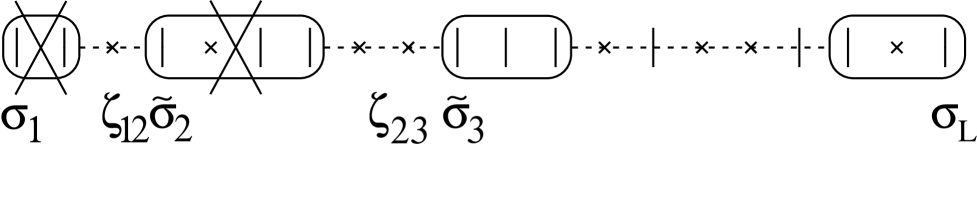
FIG. 1.: Schematic of renormalization group decimation and its use for obtaining end-to-end correlations. Clusters of spins (vertical lines) are demarcated by closed curves, decimated spins are indicated by small x’s and decimated clusters by large X’s. The dotted lines denote the effective bonds coupling the spin clusters. At a scale $\Gamma_{1}$, the cluster containing the first spin $\sigma_{1}$ was decimated with an effective bond strength $e^{-\Gamma_{1}-\zeta_{12}}$ coupling it to the left-most remaining cluster with spin $\tilde{\sigma}_{2}$. Later, at scale $\Gamma_{2}>\Gamma_{1}$, the $\tilde{\sigma}_{2}$ cluster was decimated, and the left-most remaining cluster is $\tilde{\sigma}_{3}$ as shown. The last spin, $\sigma_{L}$, is in a cluster that has not yet been decimated.

We can continue the process from both ends until there is only one remaining spin cluster with effective field

$$\tilde{h}_{E}=e^{-\Gamma_{E}}.$$ (28)

The log-correlations of the first and last spins with this last cluster are given by the $\Lambda$’s at this scale, $\Lambda_{F}(\Gamma_{E})$ and $\Lambda_{L}(\Gamma_{E})$ (for “first” and “last”) respectively. We thus have, for the end-to-end correlation function of interest,

$$\Lambda\equiv-\ln(C_{1,L})=\Lambda_{F}(\Gamma_{E})+\Lambda_{L}(\Gamma_{E}).$$ (29)

with additive errors typically of order unity. The energy gap is simply given by the scale $\Gamma_{E}$ at which the last degree of freedom—this last cluster—is decimated:

$$G\equiv-\ln(\Delta E)\approx\Gamma_{E}.$$ (30)

In order to obtain the distributions of these quantities of interest, we must keep track of the joint distribution at scale $\Gamma$ of the number of remaining clusters, $N$, their $N$ log-effective fields $\{\beta_{i}\}$, the $N-1$ log-bond strengths $\{\zeta_{i}\}$ and the contributions to the log-correlations of this stage of the RG, $\Lambda_{F}(\Gamma)$ and $\Lambda_{L}(\Gamma)$ from Eq (27), etc. A natural first guess is that, as in the infinite system, each of the couplings will be independent. But, as shown explicitly in F Section IID, this is not correct: correlations arise from the constraint that the total length is $L$. For example an anomalously small coupling, since it tends to be that of a long cluster or bond, will imply other shorter-than-typical segments with larger-than-typical couplings.

Fortunately, a modification of the naive guess of independence turns out to be correct, but it involves explicitly keeping track of the length of each segment—including the first and last, $l_{F}$ and $l_{L}$, that link $\sigma_{1}$ and $\sigma_{L}$ to the first and last remaining clusters at scale $\Gamma$. One can show that a distribution of the form [5]

$$d\mbox{Prob}[N;\Lambda_{F},l_{F};\beta_{1},l_{C1};\zeta_{1},l_{B1}\dots$$ (31)

$$\qquad\zeta_{N-1},l_{BN-1};\beta_{N},l_{CN};\Lambda_{L},l_{L}\mid L,\Gamma]$$ (32)

$$=a_{N}(L,\Gamma){\cal L}(\Lambda_{F},l_{F})d\Lambda_{F}dl_{F}R(\beta_{1},l_{C1})d\beta_{1}dl_{C1}$$ (33)

$$\qquad P(\zeta_{1},l_{B1})d\zeta_{1}dl_{B1}\times\dots\times{\cal L}(\Lambda_{L},l_{L})d\Lambda_{L}dl_{L}$$ (34)

$$\qquad\delta(l_{F}+l_{C1}+l_{B1}+\dots+l_{CN}+l_{L}-L)$$ (35)

for $N>1$ has its form preserved under renormalization if

$$a_{N}(L,\Gamma)=a(L,\Gamma)$$ (36)

is independent of $N$ with

$$\frac{1}{a}\frac{da}{d\Gamma}=\int^{\infty}_{0}\ dl[P(\zeta=0,l)+R(\beta=0,l)].$$ (37)

Note that the functions ${\cal L}$, $P$ and $R$ and all other functions that will occur later are implicitly functions of $\Gamma$ unless otherwise stated.

Initially, $N=L$ is the only term with non-zero probability, and all the $\{l_{Bi}\}$ and $\{l_{Ci}\}$ are equal to $\frac{1}{2}$, (a convention chosen for convenience). Therefore the needed solution has exactly the form of Eq (35). In terms of functions ${\cal L}$, $P$, and $R$ of the Laplace transform variable, $y$, the constraint can simply be enforced via the inverse Laplace transform

$$\raisebox{-7.74998pt}{ $\stackrel{{\scriptstyle\textstyle LT^{-1}}}{{y\to L}}$}\equiv\frac{1}{2\pi i}\int dy\ e^{yL}$$ (38)

at the end of a computation. Normalization requires that initially

$$a(L,\Gamma_{I})=\frac{1}{n_{\Gamma_{I}}}$$ (39)

(which is unity in our case) independent of $L$. ¿From Eqs. (F2.16) and (37) we then have

$$a(\Gamma)=\frac{1}{n_{\Gamma}}$$ (40)

for all $\Gamma$ where $n_{\Gamma}$ is the number density per unit length of the clusters remaining at scale $\Gamma$ in an infinite system.

The information we are interested in can be obtained from the function

$$Z(\Lambda,L,\Gamma)d\Lambda\equiv d\mbox{Prob }[\mbox{no cluster remaining}$$ (41)

$$\mbox{ and }-\ln C_{IL}=\Lambda\mid L,\Gamma].$$ (42)

When the last cluster is decimated at $\Gamma_{E}$, this will yield a contribution to $Z[\Lambda=\Lambda_{F}(\Gamma_{E})+\Lambda_{L}(\Gamma_{E}),L,\Gamma_{E}]$. In the Laplace transform variable $y$ for the lengths, using Eq (35) we have

$$J(\Lambda,y,\Gamma)\equiv\raisebox{-7.74998pt}{ $\stackrel{{\scriptstyle\textstyle LT^{-1}}}{{L\to y}}$}\ \frac{\partial Z(\Lambda,L,\Gamma)}{\partial\Gamma}$$ (43)

$$= a(\Gamma)\int d\Lambda_{F}\int d\Lambda_{L}\delta(\Lambda-\Lambda_{F}-\Lambda_{L})$$ (45)

$$R(\beta=0,y){\cal L}(\Lambda_{F},y){\cal L}(\Lambda_{L},y)$$

since the probability of decimation of the last cluster with length $l_{C}$ as $\Gamma$ is increased by $d\Gamma$ is $R(\beta=0,l_{C})d\Gamma$. The function

$$J(\Lambda,L,\Gamma=G)\equiv\raisebox{-8.61108pt}{ $\stackrel{{\scriptstyle\textstyle LT^{-1}}}{{y\to L}}$}\ J(\Lambda,y,\Gamma=G)$$ (46)

is then the joint probability distribution of $\Lambda=-\ln C_{1,L}$ and $G=-\ln\Delta E.$

The only unknown function in this process is ${\cal L}(\Lambda,l;\Gamma)$. It is just the joint distribution of the log-correlations of the first spin in a semi-infinite chain with the leftmost undecimated spin cluster at scale $\Gamma$ and the length of the bond connecting these. The Laplace transform of ${\cal L}$ in $L\to y$ and $\Lambda\to z$ is simple to analyze given the additive form of the recursion relation Eq (27). This function ${\cal L}(z,y=0)$ (i.e. ignoring the $l$ variable) is exactly the function ${\cal L}(z)$ in F Section VB. Following the analysis presented there we have

$$\frac{\partial{\cal L}(z,y)}{\partial\Gamma}={\cal L}(z,y)[P(z,y)R(\beta=0,y)-R(\beta=0,y=0)]$$ (47)

which can be integrated. Using the special family of exact solutions for $P$ and $R$, we obtain

$${\cal L}(z,y)=\frac{u(0)[z+u_{I}(y)]}{u_{I}(0)[z+u(y)]}$$ (48)

with

$$u(y)\equiv u(y,\Gamma),$$

and

$$u_{I}(y)\equiv u(y,\Gamma_{I})$$ (49)

given generally by Eqs. (F2.51) and (F2.52) which we will not need in detail here. From Eqs. (F2.46) and (F2.53) we have

$$R(\beta=0,y)=T(y),$$ (50)

defined below, and hence from Eq (43),

$$J(z,y,\Gamma)=\frac{1}{n_{\Gamma}}T(y)\left[\frac{z+u_{I}(y)}{z+u(y)}\right]^{2}\frac{u(0)^{2}}{u_{I}(0)^{2}}$$ (51)

In the scaling limit of large $\Gamma$, small $y$,

$$u(y)=\Delta(y)\coth[\Gamma\Delta(y)]-\delta$$ (52)

$$T(y)=\frac{\Delta(y)e^{\delta\Gamma}}{\sinh[\Gamma\Delta(y)]}$$ (53)

where

$$\Delta(y)=\sqrt{y+\delta^{2}}$$ (54)

with lengths measured in units of $l_{v}$. Since the scales involved initially are small, for small $y$ we have

$$u_{I}(y)\approx u_{I}(0).$$ (55)

In the scaling limit,

$$n_{\Gamma}\approx\frac{\delta^{2}}{\sinh^{2}(\Gamma\delta)}\ .$$ (56)

Since in the scaling limit we expect $\Lambda$ to typically be large, its distribution will be determined by the small $z$ behavior, so we can also write $z+u_{I}(y)\approx u_{I}(0)$; [We will consider later what has been left out by this approximation.] We now see that the $u_{I}(0)$’s cancel in the scaling limit yielding

$$J(z,y,\Gamma)=\frac{\Delta e^{-\delta\Gamma}}{\left[z-\delta+\Delta\coth(\Gamma\Delta)\right]^{2}\sinh(\Gamma\Delta)}$$ (57)

with $\Delta(y)=\sqrt{y+\delta^{2}}$ and

$$d\mbox{Prob}(\Lambda,G\mid L)=d\Lambda dG\raisebox{-7.74998pt}{ $\stackrel{{\scriptstyle\textstyle LT^{-1}}}{{y\to L}}$}\ \raisebox{-7.74998pt}{ $\stackrel{{\scriptstyle\textstyle LT^{-1}}}{{z\to\Lambda}}$}J(z,y,\Gamma=G)$$ (58)

our principal result.

C Distribution of Correlations

The distribution of the log of the end-to-end correlations, $\Lambda\equiv-\ln C_{1,L}$, can be obtained by integrating Eq (58) over $G$. The inverse Laplace transform in $z$ can be done trivially yielding

$$J(\Lambda,y,\Gamma)=\Lambda e^{\delta\Lambda-\Lambda\Delta\coth(\Gamma\Delta)}\frac{\Delta}{\sinh(\Gamma\Delta)}e^{-\delta\Gamma}\Theta(\Lambda).$$ (59)

At criticality, $\delta=0$, we can write

$$w=\frac{1}{\sinh(\Gamma\Delta)}$$ (60)

and convert the $\Gamma$ integral to a $w$ integral. The inverse Laplace transform in $y$ can then be done straightforwardly yielding a simple integral over $w$ and thereby

$$d\mbox{Prob}(\Lambda\mid L,\delta=0) = d\Lambda\frac{\Lambda}{2L}e^{-\Lambda^{2}/4L}$$ (61)

$$= d\lambda\raisebox{2.15277pt}{${\scriptstyle\frac{1}{2}}$}\lambda e^{-\lambda^{2}/4}$$ (62)

which is of scaling form in

$$\lambda\equiv\frac{\Lambda}{\sqrt{L}}.$$ (63)

Off-critical, we have not managed to compute the distribution of $\Lambda$ in closed form. But progress can be made on the moments by expanding $J$ in powers of $z$.

In the disordered phase, for small fixed $\delta>0$ and small $y$, we can expand $\Delta\approx y\delta+\frac{1}{2}\frac{y}{\delta}+\cdots$. For large $L$, one then obtains

$$\overline{\Lambda^{p}}\approx(2\delta L)^{p}$$ (64)

so that the distribution is strongly peaked around $2\delta L$. For $p=1$, Eq (64) is the first term in an expansion in powers of $\xi/L$ with the correlation length

$$\xi\approx\frac{l_{v}}{\delta^{2}}.$$ (65)

To next order we obtain

$$\overline{\Lambda}\approx 2\frac{\delta L}{l_{v}}\left\{1+\frac{\xi}{4L}\left[\ln\left(\frac{4L}{\xi}\right)+\gamma\right]+O\left(\frac{\xi^{2}}{L^{2}}\right)\right\}$$ (66)

with $\gamma\approx 0.577$, Euler’s constant. The variance of $\Lambda$ is

$$\mbox{var}(\Lambda)=\overline{(\Lambda-\overline{\Lambda})^{2}}\approx 2\frac{L}{l_{v}}+o(L)$$ (67)

with the correction probably a power of $\ln L$. In Eqs. (65)-(67) we have reinserted factors of the basic length $l_{v}$.

Note, from Eq. (66), that $\overline{\Lambda}$ is of order one for $L=\tilde{\xi}$, where

$$\tilde{\xi}={l_{v}\over 2\delta}$$ (68)

is the typical correlation length. However, the true correlation length, $\xi$ in Eq. (65), is the scale at which

$$\overline{\Lambda}(L=\xi)\sim\sqrt{\mbox{var}\,[\Lambda(L=\xi)]},$$ (69)

which is much larger. Thus the typical correlations are very small at distances of order the correlation length.

In the ordered phase, $\delta<0$, for long chains the end spins will almost have a spontaneous magnetization. We thus expect that $C_{1,L}$ will be approximately the product of two independent end-point magnetizations of an infinite system. From F section VB, we thereby obtain

$$d\mbox{Prob}[\Lambda\mid L]\approx 4\delta^{2}\Lambda e^{-2\mid\delta\mid\Lambda}d\Lambda.$$ (70)

This can also be computed from $J$ using the fact that for $\delta<0$, ${\cal L}(z,y=0,\Gamma\to\infty)$ tends to a limit as seen in F section VB.

D Energy gaps

We now turn to the distribution of energy gaps, more precisely of $G\equiv-\ln\Delta E$. This can be obtained from Eq (57) by setting $z=0$, $\Gamma=G$, and inverse Laplace transforming over $y$. For general $\delta$, we have not been able to perform this inverse transform analytically. But at the critical point the behavior again simplifies. By changing to the variable $\Delta=\sqrt{y}$, the inverse transform can be done by deforming the contour to circle a series of double poles, yielding, in terms of the scaled variable

$$g\equiv\frac{G}{\sqrt{L}}$$ (71)

$$d\mbox{Prob}[g \mid L,\delta=0]\equiv dgD(g,\delta=0)$$ (72)

$$= dg\frac{2\pi}{g^{3}}\sum^{\infty}_{n=-\infty}e^{-(n+\frac{1}{2})^{2}\pi^{2}/g^{2}}(-1)^{n}(n+\frac{1}{2})$$ (73)

$$= dg\frac{2}{\sqrt{\pi}}\sum^{\infty}_{m=-\infty}e^{-g^{2}(m+\frac{1}{2})^{2}}(-1)^{m}(m+\frac{1}{2})$$ (74)

the second expression being the Poisson resummed form of the first. We see that for large $g$,

$$D(g,\delta=0)\approx\frac{2}{\sqrt{\pi}}e^{-g^{2}/4};$$ (75)

while for small $g$,

$$D(g,\delta=0)\approx\frac{2\pi}{g^{3}}e^{-\pi^{2}/(4g^{2})}.$$ (76)

Thus the probability of both very large and very small gaps is exponentially small. The former implies that the average gap will not decay as a power of $L$. Nevertheless, from Eq(74) one can see that the integration over $g$ needed to obtain the average gap is dominated by the maximum of the integrand yielding

$$\overline{\Delta E}\sim L^{\frac{1}{6}}\exp\left(-\frac{3}{2}\left(\frac{\pi^{2}L}{2}\right)^{\frac{1}{3}}\right)$$ (77)

where we have dropped a (non-universal) prefactor. Thus at the critical point the average gap decays more slowly with $L$—indeed with a different form of $L$ dependence—than does a typical gap which has the form $\sim\exp(\rm{const.}L^{1/2})$.

In the disordered phase, the behavior for $L\gg\xi$ can be obtained by expanding $\coth(\Gamma\Delta)$ in $y$ yielding

$$J(z=0,y,\Gamma=G)\approx\frac{2\delta e^{-2\delta G}}{\left(\frac{y}{2\delta}+2\delta e^{-2G\delta}\right)^{2}}$$ (78)

valid for

$$1\ll\delta G\ll L\delta^{2}=\frac{L}{\xi}.$$ (79)

Noting that in this limit

$$n_{G}\approx 4\delta^{2}e^{-2\delta G},$$ (80)

the inverse Laplace transform simply yields

$$d\mbox{Prob}[G\mid L,\delta>0] = J(z=0,L,\Gamma=G)dG$$ (81)

$$\approx 2\delta n_{G}Le^{-Ln_{G}}dG.$$ (82)

This result has a simple interpretation [2].

For energy scales outside of the critical region, i.e. $\Gamma\gg\frac{1}{\delta}$, the remaining clusters are typically of length small compared to their separations, the latter being typically of order $1/n_{G}$. These can be thought of[2] as independent localized excitations with density $n_{G}$. Thus the probability of one of those in a sample having an anomalously small $G$ is proportional to the sample size $L$. For fixed $L$ and

$$\delta L\gg G\gg\frac{1}{\delta}\ln\left(\frac{L}{\xi}\right),$$ (83)

Eq (81) is seen to have exactly this form. Since, from Eq. (80), $n_{G}\sim(\Delta E)^{2\delta}$, the distribution of the energies of a single cluster has the form

$$\mbox{Prob}[(\Delta E)_{cluster}<\varepsilon]\sim\varepsilon^{1/z}$$ (84)

with

$$z=\frac{1}{2\delta}.$$ (85)

This interpretation [2] assumes that clusters are separated by of order $\xi$ as they indeed are at the crossover scale away from criticality, $\Gamma\sim 1/\delta$. In this regime, length $L$ corresponds to $(\mbox{energy})^{1/z}$ so that $z$ plays the role of a continuously variable dynamic exponent as discussed in F section IVA and Ref. [2]. Indeed, Eq (81) has exactly the form of a scaling function of

$$\hat{\varepsilon}\sim\varepsilon\left(\frac{L}{\xi}\right)^{z}$$ (86)

valid for $\frac{L}{\xi}\to\infty$ and $\varepsilon\to 0$ with $\hat{\varepsilon}\to$ any fixed value. Note that for extremely small gaps, $G\gg\delta L$, (for which the above results do not hold) the distribution depends on extremely rare clusters and can become less universal.

In the ordered phase, $\delta<0$, the distribution of gaps for $L\gg\xi=\frac{1}{\delta^{2}}$ can be found simply. If we guess that $G$ will typically be of order $L$, then the integral over $y$ can be done by steepest descents with the saddle point at $\Delta(y)\approx\frac{\Gamma}{2L}$. The distribution of $G$ is then found to be asymptotically Gaussian for $L\gg\frac{1}{\delta^{2}}$:

$$d\mbox{Prob}(G\mid L,\delta<0)\approx\frac{dG}{\sqrt{4\pi L}}e^{-(G-2\mid\delta\mid L)^{2}/4L}.$$ (87)

We thus have

$$\overline{G}=2\mid\!\delta\!\mid L/l_{v}$$ (88)

and

$$\mbox{var}\,G\approx 2L/l_{v}$$

where we have reinserted factors of $l_{v}$.

E Relation between correlations, gaps and couplings

We have seen that in the ordered phase the logarithm of the gap, $-G$, and in the disordered phase the logarithm of the end-to-end correlations, $-\Lambda$, both have approximately Gaussian statistics in long samples; i.e. $L\gg\xi$. Indeed, for $\delta<0$ in this limit

$$\frac{\overline{G}}{L}\approx{2\mid\!\delta\!\mid\over l_{v}}=\overline{\ln J}-\overline{\ln h}$$ (89)

and

$$\frac{\mbox{var}(G)}{L}\approx\frac{2}{l_{v}}=\mbox{var}(\ln J)+\mbox{var}(\ln h),$$

while similarly for $\delta>0$,

$$\frac{\overline{\Lambda}}{L} \approx {2\delta\over l_{v}}=\overline{\ln h}-\overline{\ln J}$$ (90)

$$\frac{\mbox{var}(\Lambda)}{L} \approx \frac{2}{l_{v}}=\mbox{var}(\ln J)+\mbox{var}(\ln h).$$ (91)

Where does this simple behavior come from? Examination of the basic recursion relations Eqs. (17) and (19) imply that at any scale, the effective field on any cluster is simply

$$\tilde{h}\approx e^{-\Sigma_{C}}$$ (92)

and the strength of any effective bond,

$$\tilde{J}\approx e^{-\Sigma_{B}}$$ (93)

with

$$\Sigma_{\rm section}\equiv\sum_{i\epsilon\ \rm{section}}(\ln h_{i}-\ln J_{i})$$ (94)

the sum running over all the original bonds or spins in the cluster ($\Sigma_{C}$) or effective bond ($\Sigma_{B}$). The last cluster to be decimated in a chain with free boundary conditions thus determines both the gap and the end-to-end correlations. If $\Sigma_{EC}$ is the sum of Eq (94) over the last to be decimated cluster and $\Sigma_{T}$ is the sum over the whole chain, i.e.

$$\Sigma_{T}=\sum_{i=1}^{L}\ln h_{i}-\sum_{i=1}^{L-1}\ln J_{i},$$ (95)

then

$$G\approx-\Sigma_{EC}$$ (96)

since the gap is the effective field on the last cluster. Likewise, the log-correlations are given by

$$\Lambda\approx\Sigma_{T}-\Sigma_{EC}$$ (97)

since, from Eq (27), $\Lambda_{F}(\Gamma_{E})$ will be the sum of $\ln h_{i}-\ln J_{i}$ over the section to the left of the last cluster and likewise $\Lambda_{F}(\Gamma_{E})$ to the right. Eqs. (96) and (97) immediately give the simple result that

$$\Lambda-G\approx\Sigma_{T}.$$ (98)

Note that the RG procedure guarantees the physical requirements that $\Lambda\geq 0$ and

$$G\geq-\ln\Omega_{I}.$$ (99)

The specific set of bonds and spins which make up the last cluster for a given sample are thus very special.

In the disordered phase for $\Gamma\gg\frac{1}{\delta}$ and $L\gg\xi$, the remaining clusters are typically small [of length $\xi$ times factors like $\ln(L/\xi)$]. Thus as $L/\xi\to\infty$,

$$\overline{\Lambda}\approx\overline{\Sigma_{T}}+o(L)$$ (100)

and

$$\mbox{var}\,\Lambda_{T}\approx\mbox{var}\,\Sigma_{T}+o(L).$$ (101)

Similarly, in the ordered phase most of the system will be in one cluster; this is the reason for spontaneous magnetization in an infinite system. Thus $\Sigma_{EC}\approx\Sigma_{T}$ so that

$$\overline{G}\approx\overline{\Sigma_{T}}+o(L)$$ (102)

$$\mbox{var}\,G\approx\mbox{var}\,\Sigma_{T}+o(L).$$ (103)

The results Eqs. (89)-(90) immediately follow.

A check on this picture can be obtained by computing the distribution of $\Lambda-G$. From Eq. (57) this is found to be purely Gaussian with the mean and variance identical (within the RG approximation) to that of $\Sigma_{T}$, as also follows directly from (98). ¿From Eqs. (95) and (98) the central limit theorem tells us that the distribution of $\Lambda-G$ is Gaussian with mean and variance given by

$$\overline{\Lambda-G} = L(\Delta_{h}-\Delta_{J})={2\delta\over l_{v}}L$$ (104)

$$\mbox{var}(\Lambda-G) = L(\mbox{var}\,h+\mbox{var}\,J)={2\over l_{v}}L,$$ (105)

where we used Eqs. (11) and (12)

We conclude this section with a note on connection to earlier work. Shankar and Murthy[4] studied the correlations of quantities, such as $\sigma^{z}_{i}\sigma^{z}_{i+1}$ or $\sigma^{x}_{i}$ which are local in fermion variables. Their results imply that, e.g.,

$$\frac{-\ln\langle\sigma^{x}_{i}\sigma^{x}_{i+r}\rangle}{\mid r\mid}\to\mid\overline{\ln h}-\overline{\ln J}\mid$$ (106)

with probability one for separation $\mid r\mid\to\infty$. Thus the asymptotic decay of “typical” correlations in the disordered phase of both $\sigma^{z}$ and $\sigma^{x}$, as well as the local energy density etc., is exponential with the same “typical correlation length”, $\tilde{\xi}$ given by Eq. (68). This prediction for the “typical correlation length” was confirmed numerically in Ref. [2].

F Average end-to-end correlations

The form of the average end-to-end correlation function, $\overline{C}_{1,L}$, can be obtained much more simply than the distribution. Crudely, the average is dominated by rare samples in which neither of the two end spins is decimated until the final scale $\Gamma_{E}$ when the last cluster, which in this case contains both $\sigma_{1}$ and $\sigma_{L}$, is decimated. ¿From the analysis we have carried out above, this corresponds simply to the $\delta(\Lambda)$ part of $J(\Lambda,L,\Gamma_{E})$. Thus up to non-universal factors arising from the high energy small scale physics, we have

$$\overline{C}_{1,L} \sim \raisebox{-7.74998pt}{ $\stackrel{{\scriptstyle\textstyle LT^{-1}}}{{L\to y}}$}\int^{\infty}_{\Gamma I}d\Gamma J(z=0,y,\Gamma)$$ (107)

$$= \raisebox{-7.74998pt}{ $\stackrel{{\scriptstyle\textstyle LT^{-1}}}{{L\to y}}$}\int^{\infty}_{\Gamma I}d\Gamma\frac{\Delta e^{-\delta\Gamma}}{\sinh(\Gamma\Delta)}\frac{1}{u^{2}_{I}(0)}.$$ (108)

At criticality, the integral over $\Gamma$ is logarithmically divergent for small $\Gamma$ yielding a $\ln(1/y)$ singularity for small $y$ corresponding to

$$\overline{C}_{1,L}\approx\frac{K}{L}$$ (109)

for large $L$, where $K$ is a non-universal constant. The sources of this non-universality are discussed in the next section.

IV Numerical Results

The numerical technique used here has been discussed previously[2, 6, 7]. It involves mapping the spin operators to fermions and diagonalizing the resulting free fermion problem. We refer to earlier work[2, 6] for details. We are able to study sizes up to $L=256$ and obtain results for about 50,000 samples. This large number is necessary in order to map out the distribution with some precision.

A End-to-end Correlations

Our data for the average end-to-end correlation function is shown in Fig. 2. The slope is about $-0.97$, close to the prediction of $-1$ in Eq. (109), and the amplitude, $K$, is close to unity.

FIG. 2.: A log-log plot of the average of the end-to-end correlation function at the critical point. The solid line is the best fit and has a slope of 0.969, close to the prediction of $-1$, see Eq. (109).

FIG. 3.: The distribution of the end-to-end correlation function at the critical point for different sizes.

The distribution of values of the end-to-end correlation function at the critical point is shown in Fig. 3. Clearly the distribution is extremely broad and becomes broader with increasing size, even on a logarithmic scale. The scaling plot in Fig. 4 shows that the data fits quite well the analytical result of Eq. (61). Note that there are no adjustable parameters in this comparison.

FIG. 4.: A scaling plot of the distribution of the end-to-end correlation function at the critical point. The solid line is the analytical result in Eq. (61), $P(\lambda)=(\lambda/2)\exp(-\lambda^{2}/4)$.

Fig. 5 shows the region near $\lambda=0$ with a linear vertical scale. Whereas the data for smaller sizes appear to have a finite intercept at $\lambda=0$ this decreases for larger sizes consistent with the analytic prediction, Eq. (61), of a linear variation for small $\lambda$ in the scaling limit.

FIG. 5.: A blowup of the region of Fig. 4 near the origin with a linear vertical scale.

The average value in Eq. (109) arises from rare samples with exceptionally large values of the correlation function which correspond to the small $\lambda$ region of Figs. 4 and 5. We shall see that the amplitude, $K$, of the $1/L$ behavior in Eq. (109) involves both a contribution from the scaling function and a non-universal part which is not contained in the scaling function. Noting that $C_{1,L}=\exp(-\lambda L^{1/2})$, the contribution to the average from the scaling function is

$$[C_{1,L}]_{\rm av}^{\mbox{scaling part}}={1\over 2}\int_{0}^{\infty}e^{-\lambda L^{1/2}}\lambda e^{-\lambda^{2}/4}\,d\lambda.$$ (110)

The dominant contribution is for $\lambda$ small, so we can replace $e^{-\lambda^{2}/4}$ by unity, which immediately gives

$$[C_{1,L}]_{\rm av}^{\mbox{scaling part}}={1\over 2L},$$ (111)

corresponding to an amplitude, $K$, in Eq. (109) of 1/2, in disagreement with the data in Fig. 2 which gives a value of about unity. In fact, the amplitude must clearly be non-universal, because one could redefine $\sigma^{z}$ to be a multiple of itself which, from the scaling form in the logarithmic variable $\lambda$, would change this amplitude but otherwise not change the physics. Clearly then, one source of the non-universal amplitude comes from the fact that $\ln C_{1,L}$ in the scaling function could be replaced by $\ln(C_{1,L}/C_{0})$, where $C_{0}$ is a constant. The scaling regime involves the limit $\ln C_{1,L}\to-\infty$ and so the factor of $C_{0}$ is a correction to scaling (actually simply the leading correction to scaling discussed in F). Note that including the factor of $C_{0}$ shifts the scaling curves in Figs. 4 and 5 horizontally by an amount of order $1/L^{1/2}$, thus giving a finite intercept at $\lambda=0$, which is seen in Fig. 5. Although the factor of $C_{0}$ is not part of the scaling function, it does affect the average correlation function since, repeating the calculation which led to Eq. (111) with $C_{0}$ included, obviously gives

$$[C_{1,L}]_{\rm av}^{\mbox{including amplitude}}={C_{0}\over 2L}.$$ (112)

FIG. 6.: A scaling plot of the distribution of energy gaps at the critical point. The solid line, which fits well, is a plot of Eq. (74) of the text.

The factor of $C_{0}$ is not the only non-scaling contribution to the amplitude. In particular, we can go back and look at the non-scaling parts of the distribution that arise from $J(z,y,\Gamma)$ in Eq. (51). The scaling limit involved neglecting $z$ with respect to $u_{I}(y)$ in the numerator of the factor in parenthesis in Eq. (51). But for large $z$, which determines the behavior for small $\Lambda$, i.e. large $C_{1,L}$, we should take the quantity in parentheses equal to unity. As discussed earlier this corresponds to situations in which neither the spin cluster containing $\sigma_{1}$ nor that containing $\sigma_{L}$ is ever decimated: i.e. both end spins remain active until the scale $\Gamma_{E}$ at which the last cluster, which in this case contains both $\sigma_{1}$ and $\sigma_{L}$, is decimated. The probability of this occurring is of order $1/L$ arising from the $u_{I}(0)$’s in Eq. (109) but with a non-universal coefficient.

Thus we see that the mean correlations have various contributions of order $1/L$ each with coefficients which depend on the high energy small scale details that are not treated correctly in our RG analysis.

B Gaps

In addition to calculating the end-to-end correlation function, we have also determined the energy gap at the critical point and show a scaling plot of the results in Fig. 6. The agreement with the prediction in Eq. (74) is good.

FIG. 7.: Data for the distribution of $\ln(\Delta E)-\ln(C_{1,l})$, both at and away from the critical point, $(\delta=0$), showing that it is a Gaussian with mean and variance given by Eq. (105) as expected. Note that $l_{v}=1$ for the distributions used here, see Eq. (14).

C Results Away from Criticality

Finally, we have also obtained some results away from the critical point. A particularly simple prediction is that $\ln(\Delta E)-\ln C_{1,L}$ should equal $\Sigma_{T}\equiv\sum_{i=1}^{L}\ln h_{i}-\sum_{i=1}^{L-1}\ln J_{i})$, defined in Eq. (98), for each sample and hence its distribution should be a Gaussian with mean $2\delta L/l_{v}$ and variance $2L/l_{v}$ for all values of $\delta$, see Eqs. (95) and (105). This works very well as shown in Fig. 7, where the solid line is the predicted Gaussian. Indeed, we find that, as expected, Eq. (95) holds for each sample. In Figs. 8-10 we have plotted $\ln(\Delta E)-\ln C_{1,L}$ against $\Sigma_{T}$ for $L=32$ and three values of $\delta$. As expected the data all lie close to the curve $y=x$, indicated by the dashed line.The small deviations presumably come from corrections to the asymptotic form obtained from the RG equations.

FIG. 8.: Results for $\ln(\Delta E)-\ln C_{(}{1,L})$ against $\Sigma_{T}\equiv\sum_{i=1}^{L}h_{i}-\sum_{i=1}^{L-1}J_{i}$ for $L=32$ at the critical point. Each point is the result for a single sample and data for 1000 samples are shown.

FIG. 9.: As for Fig. 8 but for $\delta=0.203$ in the paramagnetic phase.

FIG. 10.: As for Fig. 8 but for $\delta=-0.178$ in the ferromagnetic phase.

V Conclusions

In this paper we have studied the probability distributions of two simple properties of finite length random transverse field Ising chains at and near the critical point. In the critical regime, the natural scaling variables are the logarithms of the gap and the end-to-end correlation function divided by the square root of the length, $L$. The distributions of these properties have been computed explicitly in the scaling limit and the results agree well with numerical computations. As noted earlier, [1, 2], the average correlation function is dominated by rare samples for which the end spins have correlations of order unity; interestingly, the information about these rare events is contained, up to non-universal prefactors, in the scaling function of the distribution of $\ln C_{1,L}/\sqrt{L}$.

Although the distribution of the bulk correlation functions are much harder to compute analytically, we expect that the same general behavior will obtain for them: At the critical point, $\lambda=-\ln C_{0,r}/\sqrt{r}$ is the natural scaling variable and the mean correlations are dominated by a power law singularity in the distribution at small $\lambda$ which causes the average correlations to decay as $r^{-(3-\sqrt{5})/2}$. Off critical, the typical and average correlations both decay exponentially but with the (true) correlation length of the average correlations diverging more rapidly than the “typical correlation length” [1, 2].

This behavior is in striking contrast to that at conventional random critical points. If randomness is relevant at a classical random critical point, then the natural variable for the distribution of correlations is $\alpha=-\ln C_{0,r}/\ln r$ with [8]

$$d\mbox{Prob}(\alpha)\sim e^{-\ln r~{}f(\alpha)}d\alpha,$$ (113)

a type of distribution sometimes called ”multifractal”, although in terms of the log-correlations variable it is quite simple. The typical log-correlations are thus $\alpha_{typ}\ln r\pm O(\sqrt{\ln r})$ with $f(\alpha_{typ})=0$ the minimum value of $f$ ; i.e. they are not very broadly distributed. Nevertheless, the average correlations are dominated by rare pairs of spins and decay as a power law with exponent $\alpha_{av}<\alpha_{typ}$. Off critical, the typical and average correlations decay with different correlation lengths but the latter is only longer than the former by a constant factor.

The differences between conventional non-random quantum critical points and the random transverse field Ising chain are even more dramatic if one considers the decay of correlations in the imaginary time direction. Instead of the gap scaling as a power of the length as at conventional quantum critical points, here the logarithm of the gap scales as a power of the length but with the ratio being broadly distributed. This implies that even the log-correlations in imaginary time will be extremely broadly distributed since they will typically behave as $-\tau\ln\Delta E_{local}$ with $\Delta E_{local}$ loosely defined as the local gap. A numerical study of time-dependent correlations has been given in Ref. [6]. It would also be interesting to explore these temporal correlations in detail analytically.

At this point, it is natural to ask how broad is the class of random quantum phase transitions for which the behavior is qualitatively similar to that found here. In one dimension, the phenomena are very general. Indeed, one-dimensional random quantum Potts models [10] are in exactly the same universality class for all $q$ and some—but not all—other transitions in random quantum magnetic chains have many similar features [9].

In higher dimensions, the situation is less clear. Simulations on quantum spin glasses in two and three dimensions[11, 12] have suggested fairly conventional scaling. However, recent simulations [13, 14] of the two-dimensional random quantum Ising ferromagnet, for which larger sizes and better statistics can be obtained, indicate that most of the features found in one-dimension also apply to this case. The possibility that some strongly random quantum critical points in higher dimensions share some of the exotic features of the random transverse field Ising chains is quite intriguing.

A

In this appendix, we briefly consider the distribution of the gap in long chains with periodic boundary conditions like those used in Ref. [2]. Note that in such systems, as in bulk systems, the distributions of correlations are much more difficult to compute analytically than the end-to-end correlations for the free boundary case and we have no new results on these.

With periodic boundary conditions, it can be shown that, given $N$ remaining clusters at scale $\Gamma$ in a system of length $L$, the joint distribution of the effective couplings and their lengths is simply the conditional distribution of $N$ otherwise independent clusters and bonds in an infinite system given that their total length is $L$. As for the free boundary case, this implies correlations between the couplings which can be handled by Laplace transform methods as in the main text. The probability that there are $N$ clusters at scale $\Gamma$ can be computed from the RG equation that couples the flow of the $N$-cluster distribution and that of $N-1$ clusters when one of the $N$ bonds (or clusters) is decimated. As in the free case, $G$, minus the logarithm of the gap, is determined by the scale at which the last cluster is decimated. We obtain

$$d\mbox{Prob}(G) = L~{}dG~{}\raisebox{-7.74998pt}{ $\stackrel{{\scriptstyle\textstyle LT^{-1}}}{{L\to y}}$}\Bigl{\{}\frac{\Delta^{2}}{\sinh^{2}(G\Delta)\left[\Delta\coth(G\Delta)-\delta\right]}$$ (A1)

$$+ \int_{0}^{G}d\Gamma\frac{\Delta^{2}}{\sinh^{2}(\Gamma\Delta)}e^{-(G-\Gamma)[\Delta\coth(\Gamma\Delta)+\delta]}\Bigr{\}}.$$ (A2)

We have not been able to perform the integrations in Eq. (A2) analytically, but the asymptotic behavior of the scaling distribution at the critical point can be found. In terms of the rescaled variable $g=G/\sqrt{L}$, we find for small $g$

$$d\mbox{Prob}(g)\approx dg~{}\frac{\pi^{2}}{2g^{3}}e^{-\pi^{2}/(4g^{2})},$$ (A3)

very similar to the free-end case Eq. (76). For large $g$,

$$d\mbox{Prob}(g)\approx dg~{}\frac{g}{2}e^{-\frac{1}{4}g^{2}}$$ (A4)

again quite similar to the free-end result Eq. (76). These limiting forms are a reasonable fit to the numerical data of Ref. [2].