Magnetic Structure and NMR signal of Spin Peierls Solitons

Abstract

We compute the magnetic profile of spin Peierls solitons in a simple Heisenberg model with magneto elastic couplings, using independently the DMRG method of White and the Hartree Fock approximation. The results obtained in such a static model are incompatible with existing NMR data on CuGeO, but the distribution of averaged spins agrees qualitatively with the data. We conclude that the dynamics in the spin plus lattice system must be included in a more detailed theory of the spin Peierls transition in CuGeO.
PACS Numbers: 75.10.Jm, 75.50.Ee, 76.60.-k

I Experimental motivation, model and technique of calculation

Spin Peierls compounds such as CuGeO have solitons in their incommensurate phase [1] the magnetic profile of which can be measured by NMR techniques [2] and which must be accounted for by any theoretical model. Recently a systematic study of solitons in the Heisenberg spin Peierls model was done by Quantum Monte Carlo methods[3], with results that differ essentially from those obtained in the xy model[4]. However, these authors did not determine the distribution of spins and the corresponding NMR signal in the incommensurate phase, which are the subject of the present paper.

Here we calculate the magnetic structure of solitons in the Heisenberg Spin Peierls model via the DMRG method of White [13] and also within the Hartree Fock approximation [12]. Our (essentially exact) DMRG results in the dimerised phase agree with those of ref[3] and they are also surprisingly close to the results of a Hartree Fock calculation.

The magnetic profiles in the incommensurate phase that we compute by Hartree Fock disagree with those reconstructed from NMR data [2]. However, if we eliminate the oscillations in these profiles by averaging over even and odd sites, we find spin distributions that agree qualitatively with those obtained by NMR in ref[[2]].

The spin gap Peierls in CuGeO and similar materials [1] may be due to (i) magnetoelastic couplings [6] and/or (ii) interactions among the chains [11]. We consider the simplest realisation of case (i):

$$H = \sum_{n}J_{n,n+1}\overrightarrow{s}_{n+1}\overrightarrow{s}_{n}+\frac{\kappa}{2}\sum\left(\Delta J_{n+1,n}\right)^{2}+\mu B\sum_{n}s_{n}^{z}$$ (1)

$$J_{n,n+1} = 1+\Delta J_{n,n+1}$$ (2)

$\overrightarrow{s}_{n}$ are spin $1/2$ operators, all energies are measured in units of $J$ and $\kappa$ is the only parameter of this model. The $\Delta J_{n,n+1}$ are due to elastic deformations $\Delta J_{n,n+1}\sim(x_{n}-x_{n+1})$ the fluctuations of which are thought to be stabilised by inter chain interactions and which are treated classically. This approximation ignores the competing energy scales of phonons [8] and magnons for CuGeO (an attempt to go beyond the static approximation was undertaken in, for example, [9]). We also ignored second nearest neighbour exchange couplings that might be needed in a realistic model of CuGeO [7]. The stationary point of $<H>$ with respect to the deformations $\Delta J_{n,,n+1}$ is given by

$$\Delta J_{n,,n+1} = -\frac{1}{\kappa}<\overrightarrow{s}_{n}\overrightarrow{s}_{n+1}>+const$$ (3)

$$\sum\Delta J_{n,n+1} = 0$$ (4)

and this inhomogenous classical background $\Delta J_{n,n+1}$ is the key difficulty in tackling the Spin Peierls Hamiltonian of eq(1). We use the DMRG method of White in the original spin variables, while for Hartree Fock we use the Jordan-Wigner transform [10] of eq(1):

$$s_{n}^{+} = \prod_{k=1}^{n-1}\left(\psi_{k}^{+}\psi_{k}-\psi_{k}\psi_{k}^{+}\right)*\psi_{n}^{+}\mbox{, }s_{n}^{z}=\frac{1}{2}\left(\psi_{n}^{+}\psi_{n}-\psi_{n}\psi_{n}^{+}\right)$$ (5)

$$H_{spin} = \sum_{n}J_{n+1,n}*\left(\frac{1}{2}\psi_{n+1}^{+}\psi_{n}+h.c.+s_{n}^{z}s_{n+1}^{z}\right)+\mu B\sum_{n}s_{n}^{z}$$ (6)

As usual, the Hartree Fock (HF) approximation [12] is given by an energy functional

$$E(\rho) = <H_{spins}>$$ (7)

$$= \sum J_{n,n+1}\left[(s_{n+1}^{z}s_{n}^{z}-(\rho_{n,n+1}-\frac{1}{2})(\rho_{n+1,n}-\frac{1}{2})+\frac{1}{4}\right]+\mu B\sum s_{n}^{z}\mbox{ }$$ (8)

$$\mbox{ }s_{n}^{z}\mbox{ } = \rho_{n,n}-\frac{1}{2}$$ (9)

plus a consistency condition

$$\rho_{mn}=<\psi_{m}^{+}\psi_{n}>\mbox{, }H_{eff}=\sum_{m,n}\left(\frac{\delta E}{\delta\rho}\right)_{mn}\psi_{m}^{+}\psi_{n}$$ (10)

II First tests of our methods

To test our DMRG [13] and HF approaches, we consider the ground state energy of eq(1) for prescribed alternating dimerisation $\Delta J$ at $B=T=\kappa=0$. In the HF calculation there is an oscillating effective coupling $K_{n,n+1}=K+\Delta K(-)^{n}$ that reflects oscillations in $J_{n,n+1}=1+\Delta J(-)^{n}$ and that includes oscillations of the Hartree Fock variables. We find (details are given in an appendix)

$$K = s+\Delta s\Delta J\text{, }\Delta K=s\Delta J+\Delta s$$ (11)

$$\Delta s = \frac{2\Delta K}{\pi K}{\cal D}\text{, }s=1+\frac{2}{\pi}\left({\cal K}-{\cal D}\right)$$ (12)

$$\frac{E(\rho)}{volume} = -\frac{1}{4}\left(s^{2}+\Delta s^{2}+2\Delta Js\Delta s-1\right)$$ (13)

where ${\cal D}$ ,${\cal K}$ are standard elliptic functions with modulus $\kappa=\sqrt{1-\left(\frac{\Delta K}{K}\right)^{2}}$ . Figure(1) displays, descending in energy, (i) the ground state energy of the renormalised xy model

$$H_{xy}=(1+\frac{1}{\pi})\sum_{n}J_{n+1,n}(s_{n}^{x}s_{n+1}^{x}+s_{n}^{y}s_{n+1}^{y})$$ (14)

(ii) the Hartree-Fock energy and (iii) the DMRG result (DMRG reproduces the Bethe Ansatz result $E_{0}=1/4-\log 2$ at $\Delta J=0$).

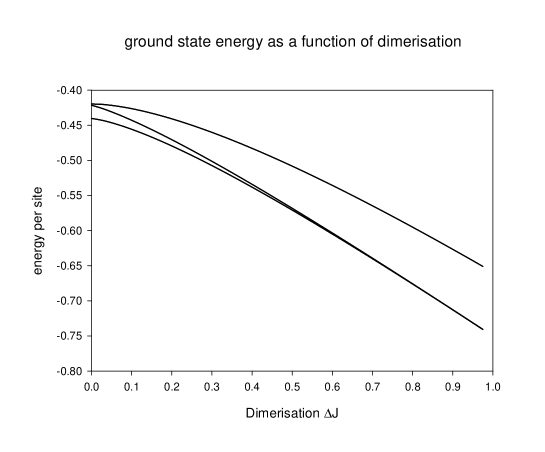
FIG. 1.: energy per site of a dimerised Heisenberg chain according to, from top to bottom, renormalised xy model, HF approximation and DMRG

The DMRG and Hartree Fock results are close and at $\Delta J=1$ where the system decouples into independent dimers, the Hartree Fock approximation is exact. Less satisfactory is the incorrect gap of the Hartree-Fock result at $\Delta J=0$ that was avoided by Bulaevski[6] by assuming the Hartree Fock parameter to be uniform along the chain. We conclude that the Hartree Fock approximation is distinct from the renormalised xy model.

Both in DMRG and HF we iterate eq(3) to converge towards the fixed point. We test this procedure on the $s=1/2$ solitons of the xy spin Peierls model of eq(14) or, equivalently the charge=$1/2$ solitons of the Peierls model of polyacetylene [5]. We recall that in the xy Spin Peierls model $<s_{x}^{z}>=0$ for half the points $[(L+1)/2]$ on a chain of odd length $L$ with periodic boundary conditions [14]. This is due to the fact that the Hamiltonian couples only even with odd points and is of the form

$$H_{xy}=\psi^{+}M\psi\mbox{, }M=\left(\begin{array}[]{ll}0&A\\ A^{+}&0\end{array}\right)$$ (15)

with a spectrum that is symmetric under $E\rightarrow-E:$

$$\left(\begin{array}[]{l}\psi_{e}\\ \psi_{o}\end{array}\right)_{E}\longleftrightarrow\left(\begin{array}[]{l}\psi_{e}\\ -\psi_{o}\end{array}\right)_{-E}$$ (16)

By the symmetry $E\leftrightarrow-E$ there are $2L$ eigenvalues of $\pm E$ plus the eigenvalue $E=0$ of the form

$$\psi_{E=0}=\left(\begin{array}[]{l}0\\ \psi_{o}\end{array}\right)$$ (17)

which alone contributes to $<s_{x}^{z}>$ and which is responsible for the vanishing of $<s_{x}^{z}>$ on half the lattice. All this is borne out by figure 2:

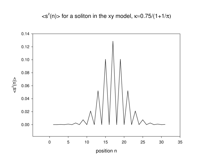
FIG. 2.: spin profile of a soliton in the xy Spin Peierls model

The magnetic profile of a soliton in the full Heisenberg spin Peierls model as obtained by DMRG and HF are given in fig.3. Clearly, this profile is quite different from that obtained in the xy Spin Peierls model.

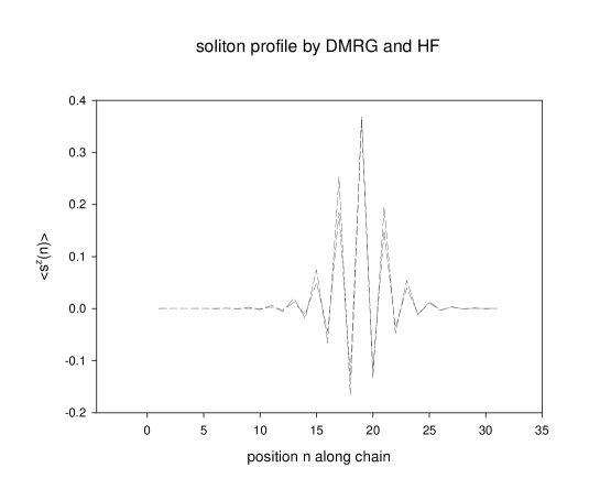
FIG. 3.: spin profile of a soliton in the Heisenberg Spin Peierls model according to HF and DMRG for $\kappa=0.75$

The DMRG result gives the symmetric profile in fig.3 and it is hard to differentiate between the two profiles.

III Solitons in the incommensurate phase and the NMR signal

Since DMRG and HF give comparable results for the spin density in the dimerised phase and since DMRG is difficult for long inhomogenous chains, we shall use HF to estimate the distribution of spins in the incommensurate phase[15].

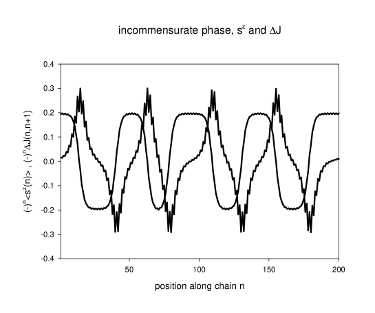
FIG. 4.: spins and lattice deformation in the incommensure phase for a chain of $L=200$, $\frac{\mu B}{J}=0.1$, $\kappa=1.5$

We crudely fix the parameter $\kappa$ by requiring that the period of the soliton structure be comparable to that observed in the NMR experiments. Consider the configuration of $\Delta J$ and $s^{z}$, multiplied by an oscillating factor, in the incommensurate phase for $L=200$, $\kappa=1.5$, $\frac{\mu B}{J}=0.1$ in fig.4.

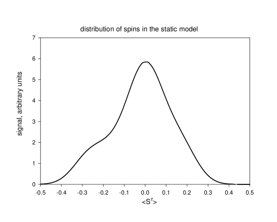
FIG. 5.: NMR signal from the static Spin Peierls model

The NMR data reflects the distribution of spins along the chain or the number of points that carry a prescribed value of spin. The configuration of spins as displayed in fig.4 (modulo an oscillating factor), gives rise to the distribution of fig.5. We see immediately that this distribution is incompatible with the NMR data of [2]: it contains positive and negative spins and the value of $s_{\max}^{z}-s_{\min}^{z}$ disagrees by a factor of $\sim 10$ with the value quoted by [2].

So we are forced to conclude that the static Heisenberg spin Peierls model for CuGeO is incompatible with the NMR data. The most plausible resolution of this

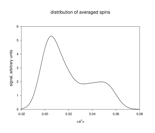
FIG. 6.: NMR signal from the distribution of averaged spins

discrepancy is that the motion of a nuclear spin in the NMR experiment averages over the dynamics of the spin plus lattice system. To mimic such an average that is, strictly speaking, outside of the domain of validity of our calculation, we take averages $\frac{1}{2}\left(s_{n}^{z}+s_{n+1}^{z}\right)$ between even and odd spins. The distribution of these average spins that is given in fig.6 is qualitatively similar to the distribution of spins in the xy model, in that the averages have one sign only. The value of $s_{\max}^{z}-s_{\min}^{z}$ for the distribution of averaged spins is of the same order as in the NMR data of [2], but the agreement with the data is only on a crude and qualitative level.

IV Conclusions

We have calculated the magnetic structure of solitons in a static Heisenberg Spin Peierls model via DMRG and the Hartree Fock approximation. Thanks to the fact that the renormalised xy model is not the HF approximation of the Heisenbergmmodel we found reasonable agreement between HF and DMRG results in the dimerised phase.

Within our static model, we obtained a spin distribution in the incommensurate phase that is incompatible with the NMR data on CuGeO. We then assumed that the NMR data reflect averages in time over fluctuating spins and lattice deformations and mimicked such internal dynamics (that is beyond the scope of our static approach) by taking averages over even and odd spins. The resulting spin distribution agrees qualitatively with the NMR data.

We conclude that the dynamics of the spin plus lattice system must be taken into account in a proper theoretical description of the Spin Peierls transition of the CuGeO system.

Acknowledgements: We are indebted to Alexander Buzdin for introducing us to the Spin Peierls problem and for showing us the NMR results. We thank Mladen Horvatic and Claude Berthier for comments on their data and Sergei Brasovskii, Lev Bulaevski and Kazumi Maki for comments on the theory. We also thank Goetz Uhrig for calling our attention to the QMC calculatios of ref[3] that we had been unaware of.

V Appendix

To correct an error in the litterature, we give the details of the Hartree Fock calculation in the dimerised phase i.e. for prescribed and uniform $\Delta J$ with $B=T=0=<s_{n}^{z}>=\rho_{n,n}-\frac{1}{2}=0$, see eq(7):

$$H_{eff} = \sum\frac{1}{2}K_{n,n+1}\psi_{n+1}^{+}\psi_{n}+h.c.$$ (18)

$$K_{n,n+1} = J_{n,n+1}*s_{n,n+1}\mbox{, }s_{n,n+1}=1-2\rho_{n,n+1}=1-2<\psi_{n}^{+}\psi_{n+1}>$$ (19)

$$E(\rho) = -\frac{1}{4}\sum J_{n,n+1}\left(s_{n,n+1}s_{n+1,n}-1\right)$$ (20)

We are interested in alternating couplings:

$$J_{n,n+1} = 1+\Delta J(-)^{n}$$ (21)

$$K_{n,n+1} = J_{n,n+1}s_{n,n+1}=K+\Delta K(-)^{n}$$ (22)

$$\Delta K = s\Delta J+\Delta s\mbox{, }K=s+\Delta J\Delta s$$ (23)

$$E(\rho) = -\frac{1}{4}volume*\left(s^{2}+\Delta s^{2}+2\Delta Js\Delta s-1\right)$$ (24)

Fourier transforming the effective Hamiltonian and diagonalising it

$$H_{eff} = \frac{1}{2}\sum\left(K+\Delta K(-)^{n}\right)\psi_{n+1}^{+}\psi_{n}+h.c..$$ (25)

$$= \sum_{|p|<\pi/2}\Lambda(p)\left[-\alpha^{+}(p)\alpha(p)+\beta^{+}(p)\beta(p)\right]$$ (26)

$$\Lambda = \sqrt{K^{2}\cos^{2}p+\Delta K^{2}\sin^{2}p}$$ (27)

$$\psi(p) = u(p)\alpha(p)+v^{*}(p)\beta(p)$$ (28)

$$\psi(p+\pi) = v(p)\alpha(p)-u^{*}(p)\beta(p)$$ (29)

we find two consistency conditions:

$$\rho_{2n,2n+1} = <\psi_{2n}^{+}\psi_{2n+1}>=t+\Delta t$$ (30)

$$\rho_{2n+1,2n+2} = <\psi_{2n+1}^{+}\psi_{2n+2}>=t-\Delta t$$ (31)

$$t = <\sum_{|p|<\pi/2}e^{ip}\left[u^{*}(p)u(p)-v^{*}(p)v(p)\right]=-\frac{1}{\pi}\left({\bf K}-{\bf D}\right)$$ (32)

$$\Delta t = <\sum_{|p|<\pi/2}\left[u^{*}(p)v(p)-v^{*}(p)u(p)\right]e^{ip}=-\frac{\Delta K}{\pi K}{\bf D}$$ (33)

$$\kappa = \sqrt{1-\left(\frac{\Delta K}{K}\right)^{2}}$$ (34)

At $T=B=0$ both conditions can be combined into one fixed point equation for $\frac{\Delta s}{s}$:

$$s = 1-2t\text{, }\Delta s=-2\Delta t$$ (35)

$$\Delta K/K = \frac{\Delta J+\Delta s/s}{1+\Delta J\Delta s/s}$$ (36)

$$\Delta s = \frac{2\Delta K}{\pi K}{\cal D}\mbox{, }s=1+\frac{2}{\pi}\left({\cal K}-{\cal D}\right)$$ (37)

$$\rightarrow \frac{\Delta s}{s}=\frac{\frac{2\Delta K}{\pi K}{\cal D}}{1+\frac{2}{\pi}\left({\cal K}-{\cal D}\right)}$$ (38)

From $\{\Delta s,s\}$ we can compute the ground state energy $E(\Delta J)$. The astonishing quality of the HF calculation raises the challenge of going beyond this approximation in a controlled way.

REFERENCES

- [1] For a review, see J. P. Boucher, L. P. Regnault, J. Phys. I, France 6 (1996) 1939
- [2] Y. Fagot-Revurat, M. Horvatic, C. Berthier, P. Segransan, G. Dhalenne, and A. Revcolevschi, Phys. Rev. Lett. 77 (1996) 1861.
- [3] A. E. Feiguin, J. A. Riera, A. Dobry and H. A. Ceccatto, cond-mat/9705205
- [4] M. Fujita, K. Machida, J. Phys. C. 21 (1988) 5813.
- [5] W. P. Su, J. R. Schrieffer and A. J. Heeger, Phys. Rev. B 22 (1980) 2099.
- [6] L. Bulaevski, JETP 16(1963) 684, JETP 17(1963) 685; E Pytte, Phy Rev. B10 (1974) 4637; A. I. Buzdin, M.L. Kulic, V. V. Tugushev, Solid. State Comm. 48 (1983) 483; M. C. Cross and D. Fisher, Phys. Rev. B 19 (1997) 402.
- [7] K. Fabricius, A. Kluemper, U. Loew, B. Buechner and T. Lorentz, cond-mat/9705036.
- [8] M. Braden, Phys. Rev. B 54, (1996)1105
- [9] G. Uhrig, ”Nonadiabatic approach to the spin Peierls transition”, cond-mat/9801185
- [10] P. Jordan and E. Wigner, Z. Phys. 47 (1928) 631.
- [11] F. H. L. Essler, A. M. Tsvelik and G. Delfino, Cond Mat/9705196.
- [12] V. I. Fock, Z. Phys. 61 (1930) 126; D. J. Thouless, ”The Quantum Mechanics of Many Body Systems ”, Academic Press 1961.
- [13] S. R. White, Phys. Rev. Lett. 69 (1992) 2863, Phys. Rev. B 48 (1993) 10345.
- [14] J. S. Bell and R. Rajaraman, Nucl. Phys. B 220 (1983) 1.
- [15] A systematic study of the incommensurate phase by DMRG methods will be given by Yann Meurdesoif in collaboration with Alexander Buzdin.