$XY$ models with disorder and symmetry-breaking fields in two dimensions

Abstract

The combined effect of disorder and symmetry-breaking fields on the two-dimensional $XY$ model is examined. The study includes disorder in the interaction among spins in the form of random phase shifts as well as disorder in the local orientation of the field. The phase diagrams are determined and the properties of the various phases and phase transitions are calculated. We use a renormalization group approach in the Coulomb gas representation of the model. Our results differ from those obtained for special cases in previous works. In particular, we find a changed topology of the phase diagram that is composed of phases with long-range order, quasi-long-range order, and short-range order. The discrepancies can be ascribed to a breakdown of the fugacity expansion in the Coulomb gas representation. Implications for physical systems such as planar Josephson junctions and the faceting of crystal surfaces are discussed.

I Introduction

We reconsider the two-dimensional $XY$ model with random phase shifts and a symmetry-breaking field, which is described by the reduced Hamiltonian

$${\cal H}=-K_{0}\sum_{{\bf r},\alpha}\cos(\nabla_{\alpha}\theta_{\bf r}-A_{{\bf r},\alpha})-H_{0}\sum_{\bf r}\cos(p\theta_{\bf r}-\phi_{\bf r}).$$ (1)

$XY$ spins $\theta_{\bf r}$ are placed on the sites $\bf r$ of a square lattice. The coupling of nearest neighbors with a spin stiffness $K_{0}\equiv J/T$ favors a relative angle prescribed by the quenched random phase shifts $A$, which we assume to be Gaussian distributed with zero mean and variance $\overline{A_{{\bf r},\alpha}^{2}}=\sigma$. The global rotation symmetry of spins is broken by the field $H_{0}$ that selects $p\in{\mathbb{N}}$ equivalent favorable directions for the spins. The model will be considered with uniform fields ($\phi=0$) and with random local orientations $\phi$ of the field.

This model describes a variety of physical systems, ranging from disordered magnets[1] to Josephson-junction arrays[2] and planar Josephson-junctions.[3] It is also closely related to surfaces of crystals with bulk disorder[4] and even to periodic elastic media such as vortex lattices in the presence of a pinning potential,[5, 6] two-dimensional crystals with quenched impurities[7] or adsorbates on disordered substrates.[8, 9]

The study of the above and related models started already decades ago. We briefly recall some marked steps in its history to provide the background for the present work. The $XY$ model in the absence of disorder and magnetic fields exhibits the Kosterlitz-Thouless (KT) transition from a phase with quasi-long-range order (QLRO, i.e., algebraic decay of the spin-spin correlation) to short-range order (SRO, i.e., exponential decay of the spin-spin correlation) at $K_{\infty}=2/\pi$,[10, 11, 12] where the effective spin stiffness $K_{\infty}\lesssim K_{0}$ is renormalized by thermal fluctuations. The transition was identified with an unbinding of vortex pairs. Weak uniform fields have been included by José, Kadanoff, Kirkpatrick, and Nelson.[13, 14] For $p>4$ they found that the phase with QLRO is stable against such fields over a temperature range $8\pi/p^{2}<K_{\infty}^{-1}<\pi/2$ and that weak fields become relevant at low temperatures $K_{\infty}^{-1}<8\pi/p^{2}$ where they stabilize long-range order (LRO, i.e. finite magnetization). For $p<4$ the transition resulting from the competition between the ordering tendency of the magnetic field and the disordering tendency of the thermal fluctuations could not be captured by a KT-like approach.

Houghton, Kenway, and Ying[15] found the phase with QLRO to be unstable to magnetic fields with random orientation only for $K_{\infty}^{-1}<4\pi/p^{2}$. Accordingly, a phase with QLRO can be stable within a finite temperature range $4\pi/p^{2}<K_{\infty}^{-1}<\pi/2$ provided $p>2\sqrt{2}$. Their study was extended by Cardy and Ostlund[16] (CO) to address the nature of the phase transitions and of the low-temperature phase. Their analysis implied that randomness of the direction of the magnetic field effectively generates a new type of disorder on large scales (in the sense of a renormalization group), namely random phase shifts $A$.[17]

Rubinstein, Shraiman, and Nelson[1] (RSN) examined the $XY$ model with random phase shifts in the absence of fields. They found QLRO to be stable against disorder below a certain critical strength and a phase diagram with reentrant shape. Paczuski and Kardar[18] (PK) added uniform fields and obtained a phase diagram composed of various phases with LRO, QLRO, and SRO. The transitions between these phases showed multiple reentrance.

Recent advance in the understanding of the bond-disordered model without fields has led to a revised nonreentrant phase diagram, where the phase with QLRO turned out to be more stable than found by RSN.[19, 20, 21, 22, 23] The earlier underestimation of the order in the system was caused by a subtle breakdown of the fugacity expansion in the Coulomb gas representation of the model at low temperatures.[24, 25] This breakdown was overcome in these recent approaches by nonperturbative techniques. The features of the revised phase diagram have been confirmed by numerical simulations.[26, 27]

The breakdown of the fugacity expansion is likely to affect all problems involving random phase shifts. In particular one has to ask how the structure of the phase diagram, the nature of the phases and the nature of the phase transitions are modified. It is also important to examine whether a similar breakdown occurs in a perturbative treatment of the fields. The purpose of the present work is to reexamine model (1) in view of these questions.

The method of our choice is a mapping of model (1) on two coupled Coulomb gases, “vortices” and “charges” (Sec. II). Thereby we take a pre-averaging over disorder using the replica trick. We establish renormalization group flow equations for the model parameters to capture the large scale properties of the system (Sec. III). From the evaluation of these flow equations (Sec. IV) we obtain results that are significantly different from those obtained by CO and PK for the special cases of ferromagnetic bonds with random fields and bond disorder with uniform fields. Our phase diagrams are illustrated in Fig. 1 for these two previously examined special cases. We conclude with a discussion of our results and of consequences for physical realizations of the $XY$ model (Sec. V). Appendices with some calculational details and a dictionary for a translation of notations from previous works to the present work are included.

II Model transformations

In this Section we specify the stochastic properties of the random phase shifts considered subsequently. In addition, we transfer randomness in the orientation of the symmetry-breaking fields to the random phase shifts such that we need to deal only with (correlated) bond disorder. The latter model is then mapped onto two coupled Coulomb gases. Eventually we arrive at a replica representation of the model that serves as basis for our further analysis.

A Disorder specification

In order to be able to treat the model irrespectively of a randomness in the local field orientation, we decompose the field ${\bf A}\equiv\{A_{\alpha}\}$ in Fourier space into its longitudinal and transverse component,

$${\bf A} = {\bf A}^{L}+{\bf A}^{T},$$ (3)

$$A^{L}_{{\bf k};\alpha} = \sum_{\beta}P^{L}_{{\bf k};\alpha,\beta}A_{{\bf k};\beta}\equiv\sum_{\beta}\frac{k_{\alpha}k_{\beta}}{k^{2}}A_{{\bf k};\beta},$$ (4)

$$A^{T}_{{\bf k};\alpha} = \sum_{\beta}P^{T}_{{\bf k};\alpha,\beta}A_{{\bf k};\beta}\equiv\sum_{\beta}\left(1-\frac{k_{\alpha}k_{\beta}}{k^{2}}\right)A_{{\bf k};\beta}.$$ (5)

Both components (polarizations $\Pi=L,T$) are supposed to be Gaussian distributed with zero average and to have variances (over-lining denotes averaging over quenched disorder)

$$\overline{A^{\Pi}_{{\bf k};\alpha}A^{\Pi}_{{\bf k}^{\prime};\beta}}=\sigma^{\Pi}P^{\Pi}_{{\bf k};\alpha,\beta}\delta({\bf k}+{\bf k}^{\prime}),$$ (6)

where we explicitly allow for $\sigma^{L}\neq\sigma^{T}$. Then the random phase shifts have a variance $\sigma=(\sigma^{L}+\sigma^{T})/2$ and are in general correlated in space. Only in the special case $\sigma^{L}=\sigma^{T}$ the phase shifts are uncorrelated on different bonds of the lattice.

Neglecting the effect of vortices and fields completely, the spin-spin correlation (angular brackets denote a thermal average for a fixed disorder realization)

$$\Gamma_{p}({\bf r})\equiv\overline{\langle\cos[p\theta_{\bf r}-p\theta_{\bf 0}]\rangle}$$ (7)

can be calculated in the spin-wave approximation and is found to decay algebraically,

$$\Gamma_{p}({\bf r})\sim r^{-\eta},$$ (8)

with an exponent $\eta=(p^{2}/2\pi)(1/K+\sigma^{L})$. In this approximation $\eta$ depends only on the longitudinal disorder. As in Ref. [16] we will also examine correlations of the Edwards-Anderson order parameter

$$\psi^{ab}({\bf r}) \equiv e^{i\theta^{a}_{\bf r}-i\theta^{b}_{\bf r}}$$ (10)

$$\overline{\langle{\psi^{ab}}^{*}({\bf r})\psi^{ab}({\bf 0})\rangle} \sim r^{-\overline{\eta}}$$ (11)

between different replicas $a\neq b$ of the system. In the spin-wave approximation the exponent $\overline{\eta}=1/\pi K$ is completely independent of disorder.[16]

B Random fields

A convenient way of dealing with the randomness in the local field orientation $\phi$ is to eliminate the angles $\phi$ in favor of modified phase shifts $\tilde{\bf A}={\bf A}-{\mathchoice{{\hbox{\boldmath$\displaystyle\nabla$}}}{{\hbox{\boldmath$\textstyle\nabla$}}}{{\hbox{\boldmath$\scriptstyle\nabla$}}}{{\hbox{\boldmath$\scriptscriptstyle\nabla$}}}}\phi/p$ by a substitution $\theta=\tilde{\theta}+\phi/p$ . This transformation leaves the thermodynamic partition sum invariant, i.e.,

$$Z(\{{\bf A}\},\{\phi\})\equiv\int{\cal D}\theta\ e^{-{\cal H}}=Z(\{\tilde{\bf A}\},\{0\}).$$ (12)

Therefore, the existence and location of phase transitions in the phase diagram are not affected by this manipulation. In contrast, spin correlation functions are not invariant and can display qualitatively different large-scale behavior before and after the transformation.

In order to restrict our analysis of random phase shifts to those with correlations (6) even after the transformation, we limit the possible distributions of the angles $\phi$ to those having a Gaussian distribution with correlations

$$\overline{\phi_{\bf k}\phi_{{\bf k}^{\prime}}}=\Delta\frac{1}{k^{2}}\delta({\bf k}+{\bf k}^{\prime}).$$ (13)

Only such random orientations are transformed by the above mapping into longitudinal phase shifts with a variance

$$\tilde{\sigma}^{L}=\sigma^{L}+\frac{\Delta}{p^{2}}.$$ (14)

Equation (13) implies correlations $\overline{(\phi_{\bf r}-\phi_{\bf 0})^{2}}\approx(\Delta/\pi)\ln r$ for $r\gg 1$ in real space. However, in the limit $\Delta\to\infty$ the relative fluctuations even of neighboring angles are that large that they can be considered practically as uncorrelated since they enter the Hamiltonian only modulo $2\pi$. In this sense the examination of the model (1) with random phase shifts and uniform field effectively includes the model with random symmetry-breaking fields in the limit $\sigma^{L}\to\infty$.

C Coulomb gas representation

We apply standard techniques[13] to map model (1) onto a Coulomb gas. For this purpose we first use the Villain approximation[28] to replace both cosines in Eq. (1) by a slightly different periodic potential and obtain an effective Hamiltonian

$${\cal H} = \frac{K}{2}\sum_{\bf r}({\mathchoice{{\hbox{\boldmath$\displaystyle\nabla$}}}{{\hbox{\boldmath$\textstyle\nabla$}}}{{\hbox{\boldmath$\scriptstyle\nabla$}}}{{\hbox{\boldmath$\scriptscriptstyle\nabla$}}}}\theta_{\bf r}-{\bf A}_{\bf r}+2\pi{\bf M}_{\bf r})^{2}$$ (16)

$$+\frac{H}{2}\sum_{\bf r}(p\theta_{\bf r}+2\pi m_{\bf r})^{2}.$$

The partition sum of this effective model contains not only the integration over the angles $\theta$ but also a summation over the integer-valued vector field ${\bf M}$ and the integer-valued scalar field $m$. The parameters of this effective model are related to the original parameters by $K=f(K_{0})$ and $H=f(H_{0})$ through the function [28, 13]

$$f(x)\approx\left\{\begin{array}[]{ll}|x|&\quad{\rm for}\quad x\gg 1,\\ -1/\ln(x^{2}/4)&\quad{\rm for}\quad x\ll 1.\end{array}\right.$$ (17)

Since we are mainly interested in the stability of the phase with QLRO (i.e., $K_{0}\gtrsim 1$) to symmetry-breaking fields (i.e., $H_{0}\ll 1$), we effectively operate in the limiting cases $K\approx K_{0}$ and $H\approx-1/\ln(H_{0}^{2}/4)$.

For small $H$ the sum over $m$ converges very slowly. Therefore it is of advantage to go over from the field $m$ to a conjugate integer-valued field $n$ by means of the Poisson summation formula (some calculational details are given in Appendix A). After integrating out the angles $\theta$ in the partition sum we end up with a new effective Hamiltonian for two coupled Coulomb gases. The first Coulomb gas is the gas of vortices with a vorticity $N={\mathchoice{{\hbox{\boldmath$\displaystyle\nabla$}}}{{\hbox{\boldmath$\textstyle\nabla$}}}{{\hbox{\boldmath$\scriptstyle\nabla$}}}{{\hbox{\boldmath$\scriptscriptstyle\nabla$}}}}\times{\bf M}\in{\mathbb{Z}}$. These vortices are located on the dual lattice, i.e., on plaquette centers ${\bf R}$.[13] The “charges” $n_{\bf r}\in{\mathbb{Z}}$ constitute the second Coulomb gas. These Coulomb gases are coupled to “quenched vortices” $Q_{\bf R}\equiv(1/2\pi){\mathchoice{{\hbox{\boldmath$\displaystyle\nabla$}}}{{\hbox{\boldmath$\textstyle\nabla$}}}{{\hbox{\boldmath$\scriptstyle\nabla$}}}{{\hbox{\boldmath$\scriptscriptstyle\nabla$}}}}\times{\bf A}$ and “quenched charges” $q_{\bf r}\equiv(K/p){\mathchoice{{\hbox{\boldmath$\displaystyle\nabla$}}}{{\hbox{\boldmath$\textstyle\nabla$}}}{{\hbox{\boldmath$\scriptstyle\nabla$}}}{{\hbox{\boldmath$\scriptscriptstyle\nabla$}}}}\cdot{\bf A}$, which are generated by the transverse and longitudinal components of the bond disorder respectively.

The Hamiltonian of the effective model reads

$${\cal H} = {\cal H}_{\rm v}+{\cal H}_{\rm c}+{\cal H}_{\rm vc}+{\cal H}_{\rm x},$$ (19)

$${\cal H}_{\rm v} = -\frac{p}{2}\sum_{{\bf R}\neq{\bf R}^{\prime}}\frac{2\pi K}{p}\ln|{\bf R}-{\bf R}^{\prime}|(N_{\bf R}-Q_{\bf R})(N_{\bf R^{\prime}}-Q_{\bf R^{\prime}})$$ (21)

$$+E_{\rm v}\sum_{\bf R}N_{\bf R}^{2},$$

$${\cal H}_{\rm c} = -\frac{p}{2}\sum_{{\bf r}\neq{\bf r}^{\prime}}\frac{p}{2\pi K}\ln|{\bf r}-{\bf r}^{\prime}|(n_{\bf r}-iq_{\bf r})(n_{\bf r^{\prime}}-iq_{\bf r^{\prime}})$$ (23)

$$+E_{\rm c}\sum_{\bf r}n_{\bf r}^{2},$$

$${\cal H}_{\rm vc} = ip\sum_{\bf R,r}\omega({\bf R}-{\bf r})N_{\bf R}n_{\bf r},$$ (24)

$${\cal H}_{\rm x} = -\frac{p}{2}\sum_{{\bf r}\neq{\bf r}^{\prime}}\frac{p}{2\pi K}\ln|{\bf r}-{\bf r}^{\prime}|q_{\bf r}q_{\bf r^{\prime}}.$$ (25)

It has been split into the interaction among vortices ${\cal H}_{\rm v}$, the interaction among charges ${\cal H}_{\rm c}$, the interaction between vortices and charges ${\cal H}_{\rm vc}$, and an excess term ${\cal H}_{\rm x}$. Particles of the same type interact logarithmically and the coupling between the two gases is given by the angle

$$\omega({\bf R}-{\bf r})=\arctan({\bf R}-{\bf r})$$ (26)

enclosed by their relative distance and an arbitrary reference direction in the $xy$ plane (see Appendix A for some intermediate steps). Due to the introduction of the charges by means of the Poisson summation formula there are two imaginary-valued contributions to the Hamiltonian: the coupling of thermal charges $n$ to quenched charges $q$ and the coupling of vortices $N$ to charges $n$. However, the partition sum is real-valued since the imaginary parts cancel in pairs $\exp[-{\cal H}(\{N\},\{n\})]+\exp[-{\cal H}(\{N\},\{-n\})]$.

Both gases are dilute for $K\gg 1$ and $H\ll 1$, where the core energies

$$E_{\rm v}\equiv\pi\gamma K,\ \ \ E_{\rm c}\equiv\frac{1}{2H}+\frac{p^{2}\gamma}{4\pi K}$$ (27)

are large ($\gamma\approx 1.6$ is a constant of order unity[29] emerging from the lattice Green function). Although these core energies are determined by $K$ and $H$ we will consider them formally as independent parameters in the subsequent treatment.

The partition function of this effective model (II C) reads

$$Z\equiv Z(2\pi K/p,E_{\rm v},E_{\rm c},\{Q\},\{q\})=\sum_{\{N\},\{n\}}^{\prime}e^{-{\cal H}}.$$ (28)

The primed summation is constrained by neutrality conditions

$$\sum_{\bf R}N_{\bf R}=0,\ \ \ \sum_{\bf r}n_{\bf r}=0,$$ (29)

since the real part of the energy of nonneutral configurations diverges logarithmically with the system size.

D Replication

The direct analysis of the partition sum (28) in the spirit of the KT renormalization group (RG) is prevented by the broken translation invariance in the presence of the quenched vortices and charges. Since we are aiming at the calculation of disorder-averaged quantities, such as the correlation function (7), we may perform the disorder average on the replicated partition sum already at this stage.[30]

For an integer number of replicas $n$ the Hamiltonian of the replicated system is most conveniently expressed in a vector notation, where ${\bf n}_{\bf r}\equiv\{n^{a}_{\bf r}\}$ for $a=1,\dots,n$ is a replica charge at site ${\bf r}$ and ${\bf N}_{\bf R}\equiv\{N^{a}_{\bf R}\}$ is a replica vortex at site ${\bf R}$:

$${\cal H} = {\cal H}_{\rm v}+{\cal H}_{\rm c}+{\cal H}_{\rm vc},$$ (31)

$${\cal H}_{\rm v} = -\frac{1}{2}\sum_{{\bf R}\neq{\bf R}^{\prime}}{\bf N}_{\bf R}\cdot{\bf K}_{\rm v}\cdot{\bf N}_{\bf R^{\prime}}2\pi\ln|{\bf R}-{\bf R^{\prime}}|$$ (33)

$$+\sum_{\bf R}{\bf N}_{\bf R}\cdot{\bf E}_{\rm v}\cdot{\bf N}_{\bf R}$$

$${\cal H}_{\rm c} = -\frac{1}{2}\sum_{{\bf r}\neq{\bf r}^{\prime}}{\bf n}_{\bf r}\cdot{\bf K}_{\rm c}\cdot{\bf n}_{\bf r^{\prime}}2\pi\ln|{\bf r}-{\bf r^{\prime}}|$$ (35)

$$+\sum_{\bf r}{\bf n}_{\bf r}\cdot{\bf E}_{\rm c}\cdot{\bf n}_{\bf r},$$

$${\cal H}_{\rm vc} = ip\sum_{\bf R,r}\omega({\bf R}-{\bf r}){\bf N}_{\bf R}\cdot{\bf n}_{\bf r}.$$ (36)

All parameters are incorporated in the replica-symmetric coupling matrices

$$K_{\rm v}^{ab} = K\delta^{ab}-\frac{\sigma^{T}K^{2}}{1+n\sigma^{T}K},$$ (38)

$$K_{\rm c}^{ab} = \frac{p^{2}}{4\pi^{2}}\left(\frac{1}{K}\delta^{ab}+\sigma^{L}\right),$$ (39)

$$E_{\rm v}^{ab} = \pi\gamma K_{\rm v}^{ab},$$ (40)

$$E_{\rm c}^{ab} = \frac{1}{2H}\delta^{ab}+\pi\gamma K_{\rm c}^{ab}.$$ (41)

Hamiltonian (II D) is a generalization of that given in Sec. II of CO. In the limit $\sigma^{L}\to\infty$ we retrieve their model, i.e., Eq. (35) becomes equivalent to their Eq. (2.15). Furthermore, in this limit the contribution of the charge core energy proportional to $\sigma^{L}$ enforces an additional neutrality

$$\sum_{a}n_{\bf r}^{a}=0$$ (42)

across the replicas, i.e., the weight of nonneutral configurations vanishes in the partition sum. Then the vector ${\bf n}$ can be decomposed into pairs of type $(0,\dots,0,1,0,\dots,-1,0,\dots 0)$ at every site. Such pairs correspond to the vector charges of CO. However, for finite $\sigma^{L}$ the summation over charges is not restricted by this additional neutrality condition. Note that Eq. (II D) contains an explicit coupling between vortices and charges.

E Duality

The effective model under consideration is self-dual,[13, 18] i.e., it is invariant under a mutual exchange of vortices and charges with a simultaneous substitution of parameters. For the unreplicated model (II C) these substitutions are

$${\bf R}\leftrightarrow{\bf r},\ N\leftrightarrow n,\ Q\leftrightarrow iq,\ \frac{2\pi K}{p}\leftrightarrow\frac{p}{2\pi K},\ E_{\rm v}\leftrightarrow E_{\rm c}.$$ (43)

This duality implies a relation

$$Z(2\pi K/p,E_{\rm v},E_{\rm c},\{Q\},\{q\})e^{+{\cal H}_{x}(2\pi K/p,\{q\})}=$$ (44)

$$Z(p/2\pi K,E_{\rm c},E_{\rm v},\{iq\},\{-iQ\})e^{+{\cal H}_{x}(p/2\pi K,\{-iQ\})}$$ (45)

for the partition sum,[18] which simplifies our subsequent calculations because it enables us to relate renormalization effects arising from vortex fluctuations to renormalization effects arising from charge fluctuations or vice versa. In this way PK obtained recursion relations for the bond-disordered model with field from those of RSN without field. We are going to use the same strategy starting from the corrected flow equations.[22]

We will proceed within the replica formulation (II D), where the self-duality of the model is reflected by the substitutions

$${\bf R}\leftrightarrow{\bf r},\ {\bf N}\leftrightarrow{\bf n},\ {\bf K}_{\rm v}\leftrightarrow{\bf K}_{\rm c},\ {\bf E}_{\rm v}\leftrightarrow{\bf E}_{\rm c}.$$ (46)

The excess contribution (25) to the Hamiltonian of the unreplicated system effectively modifies the action of the longitudinal disorder distribution. The duality ${\bf K}_{\rm v}\leftrightarrow{\bf K}_{\rm c}$ implies $\sigma^{L}\leftrightarrow-(4\pi^{2}K^{2}/p^{2})\sigma^{T}/(1+n\sigma^{T}K)$. The latter relation is consistent with Eq. (43) if one keeps in mind the presence of the excess term in Eq. (44). This term gives rise to the denominator $1+n\sigma^{T}K$ that becomes unity in the limit $n\to 0$ that eventually will be taken.

III Renormalization

After the Coulomb gas representation of our model has been established in the previous Section we now turn to a scaling analysis for the relevance of vortices and charges. We basically follow Kosterlitz’ RG approach [11] to the $XY$ model and its recent generalization[22] to the $XY$ model with random phase shifts. To account for magnetic fields we have to include charges and their coupling to the vortices.

Following Ref. [22] we introduce the notion of “types” of replica vortices and charges. We consider charges at site ${\bf r}$ and site ${\bf r}^{\prime}$ as being of the same or of different type if ${\bf n}_{\bf r}={\bf n}_{{\bf r}^{\prime}}$ or ${\bf n}_{\bf r}\neq{\bf n}_{{\bf r}^{\prime}}$ in analogy to the vortex types. From the core energy contribution to the Hamiltonian (II D) we identify fugacities

$$y_{\rm v}({\bf N}) = e^{-{\bf N}\cdot{\bf E}_{\rm v}\cdot{\bf N}}$$ (48)

$$y_{\rm c}({\bf n}) = e^{-{\bf n}\cdot{\bf E}_{\rm c}\cdot{\bf n}}$$ (49)

for each type of particles. Because of the replica symmetry of the matrices ${\bf E}_{\rm v}$ and ${\bf E}_{\rm c}$ different particle types have the same fugacity if they belong to the same “class,” that is, if they are of the same type after a permutation of replicas and/or an inversion of the replica vector (such as ${\bf n}_{\bf r}\to-{\bf n}_{\bf r}$).

A Scaling analysis

In the limit of vanishing field all charge fugacities (IIIb) go to zero. The relevance of a weak field can be examined by looking at the scaling behavior of the charge fugacities. As soon as the fugacity of some charge type increases under rescaling, the field constitutes a relevant perturbation. Analogously, the relevance of vortices signals the importance of topologically nontrivial spin configurations. However, while a relevance of vortices indicates a tendency to reduced spin correlations on large scales, a relevance of charges expresses a tendency to enhanced spin correlations.

A rescaling of lengths ${\bf R}\to e^{-dl}{\bf R}$ and ${\bf r}\to e^{-dl}{\bf r}$ with an infinitesimal increase on a logarithmic length scale $l$ has the following effect on Hamiltonian (II D): the angles $\omega$ are invariant but the logarithms generate additive constants, $\ln|\dots|\to\ln|\dots|-dl$. Using the neutrality conditions (29) the twofold spatial summations over these constants can be reduced to single summations. Then the rescaling effectively amounts to an additive flow of the core matrices ${\bf E}$, or equivalently to a multiplicative flow of the fugacities

$$\left.\frac{d}{dl}\right|_{\rm scal}y_{\rm v}({\bf N}) = (2-\pi{\bf N}\cdot{\bf K}_{\rm v}\cdot{\bf N})y_{\rm v}({\bf N}),$$ (51)

$$\left.\frac{d}{dl}\right|_{\rm scal}y_{\rm c}({\bf n}) = (2-\pi{\bf n}\cdot{\bf K}_{\rm c}\cdot{\bf n})y_{\rm c}({\bf n}).$$ (52)

For a finite number $n$ of replicas we can now determine the stability of QLRO to vortices and charges at given temperature $K^{-1}=T/J$ and disorder strengths $\sigma^{\Pi}$ by looking for the most relevant class of particles. We focus here on the charge sector, since the vortex sector has been covered in Ref. [22]. The most relevant charge class is the one that minimizes

$${\bf n}\cdot{\bf K}_{\rm c}\cdot{\bf n}=\frac{p^{2}}{4\pi^{2}}\left[\sum_{a}(n^{a})^{2}K^{-1}+\left(\sum_{a}n^{a}\right)^{2}\sigma^{L}\right].$$ (53)

The minimum is provided by charges of class $\uparrow$ for $\sigma^{L}<K^{-1}$ and by charges of class $\uparrow\downarrow$ for $\sigma^{L}>K^{-1}$. The class “$\uparrow$” is composed of all replica charges ${\bf n}$ that contain an elementary charge in a single replica [e.g., ${\bf n}=(0,\dots,0,\pm 1,0,\dots,0)$] and the class “$\uparrow\downarrow$” is composed of all replica charges ${\bf n}$ that contain an elementary charge in one replica and an opposite elementary charge in a second replica [i.e., the CO vector charges, such as ${\bf n}=(0,\dots,0,+1,0,\dots,0,-1,0,\dots,0)$].

Let us consider for illustration vector charges that are composed only of $s$ elementary charges, thereof $s_{\uparrow}$ are positive and $s_{\downarrow}$ are negative. The fugacity of such charges scales like

$$y_{\rm c}({\bf n})\sim\exp\left\{l\left[2-\left[(s_{\uparrow}+s_{\downarrow})K^{-1}-(s_{\uparrow}-s_{\downarrow})^{2}\sigma^{L}\right]\frac{p^{2}}{4\pi}\right]\right\}.$$ (54)

Figure 2 displays the stability boundary in the ($K^{-1},\sigma^{L}$) plane for various classes of charges, which are irrelevant on the high-temperature side of the corresponding (full) lines. Charge class $\uparrow$ is most relevant on the high-temperature side ($\sigma^{L}<K^{-1}$) and charge class $\uparrow\downarrow$ is most relevant on the low temperature side ($\sigma^{L}>K^{-1}$) of the dashed line.

There is an important difference in the scaling analysis for charges and for vortices. The region of the phase diagram, where all $n$-component charges are irrelevant, is independent of the number $n$ of replicas. In addition, the boundary of this region is invariantly given for all integer $n$ by the charge classes $\uparrow$ or $\uparrow\downarrow$ (strictly speaking, the class $\uparrow\downarrow$ exists only for $n\geq 2$). This independence on $n$ indicates that the replica limit $n\to 0$ can be taken in a very simple way. In contrast, the region where all vortices are irrelevant depends explicitly on $n$ and so does the class of the most relevant vortices at lower temperatures (see Fig. 2 of Ref. [22]). Therefore the replica limit will be easier to take for charges than for vortices. The save proceeding for both cases is to consider the collective renormalization of the physical parameters by all classes of vortices and charges, which will be carried out subsequently.

We anticipate here that through this proceeding we obtain first closed expressions for the collective effects of charges, for which the perturbative expansion in small charge fugacities can be justified a posteriori. The various terms in this expansion can again be identified with vector charge classes. The leading terms correspond to the most relevant classes identified above and the stability region (shaded area) of Fig. 2 remains unchanged.

B Screening

The renormalization of parameters on large scales due to fluctuations on small scales will now be calculated by integrating out pairs of particles from the partition sum following the approach of Kosterlitz.[11] Since our model possesses the vortex-charge duality, it is sufficient to perform the actual calculations only in one particle sector. The renormalization effects of the other sector are then obtained by a duality transformation. We adopt the results for the vortex sector directly from Ref. [22]. However, we extend these previous calculations at two points. First, we calculate the flow equations for the fugacities to higher order in the fugacities. This extension is necessary to consider the parameter renormalizations not only within the phase with QLRO, but also in the phase where magnetic fields are relevant. This requires flow equations of higher order in the charge fugacities, which we can obtain through the duality mapping only from the terms of higher order in the vortex fugacities. Second, when the vortex dipoles are integrated out in the presence of charges, they renormalize the interactions among the charges (and vice versa). This feature was naturally absent in Ref. [22], where fields were not included.

For technical convenience we allow replica vortices to take positions in the continuous space and not only on the lattice. The lattice provides only a cutoff (taken to be unity) for the minimal distance between vortices. Our present goal is to integrate out all configurations in the partition sum, where the smallest distance between two replica vortices (of any type) lies in the range $1\leq|{\bf R}_{1}-{\bf R}_{2}|<1+dl$. We follow Young’s treatment of a vector Coulomb gas,[31] which can be applied directly to our vectors ${\bf N}$. During this procedure two cases have to be distinguished: (i) the two close vortices are of opposite type, i.e., ${\bf N}_{1}+{\bf N}_{2}=0$ (in the continuous space subscripts to ${\bf N}$ denote the particle label instead of the position) and (ii) these two vortices are not of opposite type, i.e., ${\bf N}_{1}+{\bf N}_{2}\neq 0$.

In case (i), where the pair of close vortices is composed of a vortex and its antivortex, they essentially annihilate. The leading interaction with the other particles, which are approximately considered to be far away, is through the dipole moment of the pair. Because of the polarizability of this dipole moment the pair screens the interaction between the other particles.[10, 11] The screening of the interaction among vortices can be captured by a flow of the coupling

$$\left.\frac{d}{dl}\right|_{\rm scr}{\bf K}_{\rm v}=2\pi^{3}{\bf K}_{\rm v}\cdot{\bf C}_{\rm v}\cdot{\bf K}_{\rm v},$$ (55)

where

$$C_{\rm v}^{ab}\equiv-\sum_{{\bf N}\neq{\bf 0}}N^{a}N^{b}y_{\rm v}^{2}({\bf N})$$ (56)

is the replica vortex density correlation at the cutoff distance [see Eq. (13) of Ref. [22]]. Due to the angular coupling between vortices and charges there is an additional screening of the interaction among charges (see Appendix B):

$$\left.\frac{d}{dl}\right|_{\rm scr}{\bf K}_{\rm c}=-\frac{\pi}{2}p^{2}{\bf C}_{\rm v}.$$ (57)

Besides the screening of these coupling matrices, the annihilation of such dipoles changes the free energy per unit area and per replica by

$$\left.\frac{d}{dl}\right|_{\rm scr}{\cal F}=-\frac{\pi}{n}\sum_{{\bf N}\neq{\bf 0}}y_{\rm v}^{2}({\bf N}).$$ (58)

In case (ii) the two close vortices appear (in the eyes of the other particles, which are assumed to be far away) essentially as a single vortex of type ${\bf N}_{3}={\bf N}_{1}+{\bf N}_{2}$, i.e. the dominant interaction with the other particles is not given by the dipole moment of the pair but by the total vorticity. Therefore we can “replace” the two vortices by the single one, i.e., we transfer the statistical weight of the entire particle configuration to a different particle configuration, where the two close vortices 1 and 2 are replaced by a vortex of type 3 and all other particles are unchanged. By analogy with Young’s analysis[31] [leading to his Eq. (75)] we obtain

$$\left.\frac{d}{dl}\right|_{\rm scr}y_{\rm v}({\bf N})=\pi\sum_{{\bf N}_{1},{\bf N}_{2}\neq{\bf 0}}\delta_{{\bf N},{\bf N}_{1}+{\bf N}_{2}}y_{\rm v}({\bf N}_{1})y_{\rm v}({\bf N}_{2}).$$ (59)

The neutrality conditions (29) are preserved under such types of recombination.

C Flow equations

In order to establish the RG flow equations, we combine the contributions from scaling and screening. Using the duality relations (46) we infer the contributions by charge fluctuations immediately from those by vortex fluctuations that have been given above. Thus, after collecting all terms, we find the complete flow equations for the replicated system

$$\frac{d}{dl}y_{\rm v}({\bf N}) = \left(2-\pi{\bf N}\cdot{\bf K}_{\rm v}\cdot{\bf N}\right)y_{\rm v}({\bf N})$$ (62)

$$+\pi\sum_{{\bf N}_{1},{\bf N}_{2}\neq{\bf 0}}\delta_{{\bf N},{\bf N}_{1}+{\bf N}_{2}}y_{\rm v}({\bf N}_{1})y_{\rm v}({\bf N}_{2}),$$

$$\frac{d}{dl}y_{\rm c}({\bf n}) = \left(2-\pi{\bf n}\cdot{\bf K}_{\rm c}\cdot{\bf n}\right)y_{\rm c}({\bf n})$$ (64)

$$+\pi\sum_{{\bf n}_{1},{\bf n}_{2}\neq{\bf 0}}\delta_{{\bf n},{\bf n}_{1}+{\bf n}_{2}}y_{\rm c}({\bf n}_{1})y_{\rm c}({\bf n}_{2}),$$

and

$$\frac{d}{dl}{\bf K}_{\rm v} = 2\pi^{3}{\bf K}_{\rm v}\cdot{\bf C}_{\rm v}\cdot{\bf K}_{\rm v}-\frac{\pi}{2}p^{2}{\bf C}_{\rm c},$$ (66)

$$\frac{d}{dl}{\bf K}_{\rm c} = 2\pi^{3}{\bf K}_{\rm c}\cdot{\bf C}_{\rm c}\cdot{\bf K}_{\rm c}-\frac{\pi}{2}p^{2}{\bf C}_{\rm v},$$ (67)

$$\frac{d}{dl}{\cal F} = -\frac{\pi}{n}\sum_{{\bf N}\neq{\bf 0}}y_{\rm v}^{2}({\bf N})-\frac{\pi}{n}\sum_{{\bf n}\neq{\bf 0}}y_{\rm c}^{2}({\bf n}).$$ (68)

Since we establish the flow equations for an infinitesimal change of the cutoff, we assume that we can simply add vortex and charge contributions, i.e., that there are no terms mixing vortex and charge fugacities. Such a mixing could arise in principle if one implies a minimal cutoff distance not only among vortices and among charges, but also between vortices and charges. We are inclined to believe that a hard-core interaction between vortices and charges is not necessary, because we do not expect divergences related to short distances of that type: due to the imaginary-valued nature of angular coupling (24) in the Hamiltonian it seems plausible that configurations with close vortex-charge pairs give no essential contribution to the partition sum.

Since not only the original couplings ${\bf K}$ but also the particle density correlations ${\bf C}$ are replica-symmetric, this symmetry holds also for the screened couplings. Even more, the renormalized matrices ${\bf K}_{\rm v}$ and ${\bf K}_{\rm c}$ can be reexpressed in terms of renormalized parameters $K$ and $\sigma^{\Pi}$ preserving relations (II Da,b): Equations (III Ca,b) are equivalent to

$$\frac{d}{dl}K^{-1} = -2\pi^{3}C_{\rm v,con}+\frac{\pi}{2}p^{2}K^{-2}C_{\rm c,con},$$ (70)

$$\frac{d}{dl}\sigma^{\Pi} = -2\pi^{3}C_{\rm v,dis}+\frac{\pi}{2}p^{2}K^{-2}[C_{\rm c,dis}$$ (72)

$$+\sigma^{\Pi}K(2+n\sigma^{\Pi}K)(C_{\rm c,con}+nC_{\rm c,dis})].$$

Thereby the particle correlation matrices were decomposed into the “connected” and “disconnected” contributions according to

$$C^{ab}=C_{\rm con}\delta^{ab}+C_{\rm dis}$$ (73)

for both vortices and charges.

D Replica limit $n\to 0$

So far, the derivation of the RG flow equations for the replicated system have been conceptually straightforward. The less trivial part is to take the replica limit, i.e., to perform an analytic continuation for $n\to 0$.

The first step in this direction was the reduction of the ${\bf K}$ matrix flow equation to the parameter flow equations (III C). We focus on these equations, since the physical large-scale properties of our system show up in the flow of these parameters. In order to send $n\to 0$ in these flow equations, we have to overcome only one hurdle: to make $n$ an explicit parameter in the connected and disconnected correlations. Here again we follow the route of Ref. [22], where the problem was solved for the vortex correlations, and treat charges on the same footing.

One easily realizes from the flow equations for the fugacities that large vortices (charges) with $|N^{a}|>1$ ($|n^{a}|>1$) are less relevant than small vortices (charges) with $|N^{a}|\leq 1$ ($|n^{a}|\leq 1$). Therefore it is a good approximation to restrict the further calculation to the small particles (this approximation is made for simplicity, the inclusion of large particles is possible). The correlations can then explicitly be evaluated after introducing a auxiliary random variable ${\cal A}$. Its distribution is defined to be Gaussian with average $[{\cal A}]_{\cal A}=0$ and variance $[{\cal A}^{2}]_{\cal A}=1/2$ (averages over ${\cal A}$ are denoted by $[\dots]_{\cal A}$). We decompose the core energy matrices (II Dc,d) into

$$E^{ab}=E\delta^{ab}-\hat{E}$$ (74)

for vortices and charges (one specifies by adding the corresponding subscripts “v” or “c”). The initial values of $E$ given in Eq. (27) and

$$\hat{E}_{\rm v}=\frac{\pi\gamma\sigma^{T}K^{2}}{1+n\sigma^{T}K},\ \ \ \hat{E}_{\rm c}=-\frac{\gamma p^{2}\sigma^{L}}{4\pi}.$$ (75)

Next, we introduce weights (proportional to the fugacities $e^{-2E}$ of the elementary particles)

$$z_{\pm}\equiv e^{-2(E\pm{\cal A}\sqrt{2\hat{E}})},\ \ \ z\equiv 1+z_{+}+z_{-},$$ (76)

and, combining Eqs. (III) with (56) and its dual counterpart, we rewrite the correlations as

$$C^{aa} = -\left[(z_{+}+z_{-})z^{n-1}\right]_{\cal A},$$ (78)

$$C^{ab} = -\left[[(z_{+}-z_{-})^{2}z^{n-2}\right]_{\cal A},$$ (79)

where we take $a\neq b$. In this representation the number of replicas became an explicit variable that can be sent to zero, resulting in

$$C_{\rm dis} = -\left[\left(\frac{z_{+}-z_{-}}{1+z_{+}+z_{-}}\right)^{2}\right]_{\cal A},$$ (81)

$$C_{\rm con} = -\left[\frac{z_{+}+z_{-}+4z_{+}z_{-}}{(1+z_{+}+z_{-})^{2}}\right]_{\cal A}.$$ (82)

Then the replica limit of the flow equations (III C) for $K$ and $\sigma^{\Pi}$ can be taken right away, since now all dependences on $n$ are explicit.

The contributions to the flow of the free energy (III Cc) can be rewritten as[22]

$$\frac{1}{n}\sum_{{\bf N}\neq{\bf 0}}y_{\rm v}^{2}({\bf N})=\frac{1}{n}[z_{\rm v}^{n}-1]_{\cal A}\to[\ln z_{\rm v}]_{\cal A},$$ (83)

where in the last expression the replica limit has already been performed. The analogous charge contribution is obtained by duality substitutions.

E Fugacity expansion

Combining expressions (III Cc), (III C), (III D), and (83) the flow of the physical quantities $K$, $\sigma^{\Pi}$, and ${\cal F}$ can be expressed through the fugacities $z_{\pm}$ for both types of particles. According to Eq. (27) these fugacities are small for large $K$ and small $H$ and one might be tempted to simplify the expressions (III D) and (83) by a truncated expansion in these fugacities.

The early studies of the disordered $XY$ model[16, 1, 2, 18] made use of this fugacity expansion. The invalidity of this expansion was recognized later on and was considered as a possible reason for the destruction of QLRO even by infinitesimally weak disorder.[24, 25] However, it was shown recently[19, 21, 22, 23] for the model without fields that the mere breakdown of the fugacity expansion does not imply the relevance of vortices and the destruction of QLRO. In other terms: in the vortex sector the closed expressions (III D) and (83) are finite and they are to be evaluated nonperturbatively. Therefore it is a central issue of the present work to reexamine the validity of the fugacity expansion for charges that underlies Refs. [16, 18].

To be explicit let us examine the “smallness” of the charge fugacities $z_{{\rm c}\pm}$ defined in Eq. (76). In contrast to the real-valued vortex fugacities they are complex-valued since $\sqrt{\hat{E}_{\rm c}}$ is purely imaginary. Their absolute value

$$|z_{{\rm c}\pm}|=e^{-2E_{\rm c}}\approx e^{-1/H}\approx\frac{H_{0}^{2}}{4}$$ (84)

is small for weak fields independently of the disorder represented by the variable ${\cal A}$. Therefore it is safe to expand the expressions correlations (III D) for charges before performing the average over ${\cal A}$. Again, this is in sharp contrast to the case of vortices, where the fugacities become arbitrarily large in the tails of the distribution of ${\cal A}$. Thus, the mechanism that led to the failure of the fugacity expansion for vortices is not effective for charges.

Thus, we are entitled to use the fugacity expansion for charges to study the stability QLRO to weak fields. We expand the charge correlations (III D) [and analogously the source of the flow of the free energy, the dual counterpart of Eq. (83)] to second order in the fugacities $z_{{\rm c}\pm}$ and perform the average over ${\cal A}$:

$$C_{\rm c,dis} = 2y_{{\rm c}\uparrow\downarrow}^{2}-2y_{{\rm c}\uparrow\uparrow}^{2}+\cdots,$$ (86)

$$C_{\rm c,con} = -2y_{{\rm c}\uparrow}^{2}+4y_{{\rm c}\uparrow\uparrow}^{2}+\cdots,$$ (87)

$${[\ln z_{\rm c}]}_{\cal A} = 2y_{{\rm c}\uparrow}^{2}-y_{{\rm c}\uparrow\downarrow}^{2}-y_{{\rm c}\uparrow\uparrow}^{2}+\cdots$$ (88)

We have replaced the terms in the series by vector charge fugacities using the identification (III) and substituted the symbols $y_{\rm c}({\bf n})$ by the more illustrative arrow symbols. The initial values of these fugacities are given by

$$y_{{\rm c}\uparrow} = e^{-[1/2H+(\gamma p^{2}/4\pi)(K^{-1}+\sigma^{L})]},$$ (90)

$$y_{{\rm c}\uparrow\downarrow} = e^{-[1/H+(\gamma p^{2}/2\pi)K^{-1}]},$$ (91)

$$y_{{\rm c}\uparrow\uparrow} = e^{-[1/H+(\gamma p^{2}/2\pi)(K^{-1}+2\sigma^{L})]}.$$ (92)

All bare charge fugacities are determined by only three physical parameters $K$, $\sigma^{L}$, and $H$. This relation is abandoned under renormalization, where the flow of $K$ and $\sigma^{L}$ follows Eq. (III C) and where we have a whole set of flow equations (III C) for the charge fugacities instead of a single flow equation for $H$. It is interesting to note that a fugacity with $s$ arrows is of order $H_{0}^{s}$ in the original field [remember relation (17)]. This order $s=s_{\uparrow}+s_{\downarrow}$ is just the total number of positive/negative elementary charges introduced in Eq. (54) above.

Since the fugacity expansion is valid for the charges, it is legitimate to analyze the stability of QLRO by demanding that all classes of vector charges have to be irrelevant. This analysis has been performed in Sec. III A leading to the shaded stability area in Fig. 2. As long as all charges are irrelevant, the second order terms in the flow equation (III Cb) play actually no role. For a qualitative study of the flow of charge fugacities slightly inside the region where charges are relevant, we keep only the two charge classes $y_{{\rm c}\uparrow}$ and $y_{{\rm c}\uparrow\downarrow}$. This should be a reasonable approximation since it is always one of these two classes that brings about the instability of QLRO at the low-temperature border of the stability region and that represent the most relevant charge class among all classes and for all parameters, as discussed after Eq. (54). Therefore we truncate the charge fugacity flow equations (III Cb) to

$$\frac{d}{dl}y_{{\rm c}\uparrow} = [2-(p^{2}/4\pi)(K^{-1}+\sigma^{L})]y_{{\rm c}\uparrow}-2\pi y_{{\rm c}\uparrow}y_{{\rm c}\uparrow\downarrow},$$ (94)

$$\frac{d}{dl}y_{{\rm c}\uparrow\downarrow} = [2-(p^{2}/2\pi)K^{-1}]y_{{\rm c}\uparrow\downarrow}+2\pi[y_{{\rm c}\uparrow}^{2}-2y_{{\rm c}\uparrow\downarrow}^{2}].$$ (95)

However, we stress that these truncated flow equations are incomplete, i.e., these two selected fugacities are coupled to all other fugacities in the complete flow equations. We have dropped also charge class $\uparrow\uparrow$, which also brings about only quantitative modifications. Only for $\sigma^{L}=0$ they are as relevant as charges $\uparrow\downarrow$ and should be kept, e.g., to obtain the vanishing of the disconnected correlation (III Ea).

Concerning the processing of the vortex sector, we actually don’t go beyond Ref. [22]. That is, we restrict our quantitative analysis to the region, where vortices are irrelevant and the second-order terms to the vortex fugacity flow equations (III Ca) can be discarded. The linear flow equations for all $y_{\rm v}({\bf N})$ can be reduced to flow equations for $E_{\rm v}$ and $\hat{E}_{\rm v}$.[22] Avoiding a fugacity expansion, the vortex correlations $C_{\rm v}$ can be evaluated asymptotically for large length scales and can be expressed in terms of an effective vortex fugacity $y_{\rm v}$,

$$C_{\rm v,con} = -2\tau^{*}y_{\rm v}^{2},$$ (97)

$$C_{\rm v,dis} = -2(1-\tau^{*})y_{\rm v}^{2},$$ (98)

$${[\ln z_{\rm v}]}_{\cal A} = \frac{2}{\tau^{*}},$$ (99)

with a fraction of “polarizable dipoles”

$$\tau^{*}\equiv\min(1,1/2\sigma^{T}K).$$ (100)

This fraction is unity for temperatures $K^{-1}>2\sigma^{T}$ and goes to zero as the temperature drops below $K^{-1}<2\sigma^{T}$, where vortices start to freeze. The initial value and the renormalization flow of the effective fugacity is given by[22]

$$y_{\rm v}^{2} = \frac{1}{2}\left[\frac{z_{+}+z_{-}}{1+z_{+}+z_{-}}\right]_{\cal A},$$ (102)

$$\frac{d}{dl}y_{\rm v} = [2-\pi\tau^{*}K(1-\sigma^{T}\tau^{*}K)]y_{\rm v}.$$ (103)

To summarize the above derivations we collect the full set of flow equations that constitute one of our main findings:

$$\frac{d}{dl}K^{-1} = 4\pi^{3}\tau^{*}y_{\rm v}^{2}-\pi p^{2}K^{-2}y_{{\rm c}\uparrow}^{2},$$ (105)

$$\frac{d}{dl}\sigma^{\Pi} = 4\pi^{3}(1-\tau^{*})y_{\rm v}^{2}-\pi p^{2}[2\sigma^{\Pi}K^{-1}y_{{\rm c}\uparrow}^{2}$$ (107)

$$-K^{-2}y_{{\rm c}\uparrow\downarrow}^{2}],$$

$$\frac{d}{dl}y_{\rm v} = [2-\pi\tau^{*}K(1-\sigma^{T}\tau^{*}K)]y_{\rm v},$$ (108)

$$\frac{d}{dl}y_{{\rm c}\uparrow} = [2-(p^{2}/4\pi)(K^{-1}+\sigma^{L})]y_{{\rm c}\uparrow}-2\pi y_{{\rm c}\uparrow}y_{{\rm c}\uparrow\downarrow},$$ (109)

$$\frac{d}{dl}y_{{\rm c}\uparrow\downarrow} = [2-(p^{2}/2\pi)K^{-1}]y_{{\rm c}\uparrow\downarrow}+2\pi[y_{{\rm c}\uparrow}^{2}-2y_{{\rm c}\uparrow\downarrow}^{2}],$$ (110)

$$\frac{d}{dl}{\cal F} = -\frac{2\pi}{\tau^{*}}y_{\rm v}^{2}-\pi(2y_{{\rm c}\uparrow}^{2}-y_{{\rm c}\uparrow\downarrow}^{2}).$$ (111)

This set of flow equations has no longer an explicit duality between vortices and charges (even if we ignore the second-order terms in the flow equations of the charge fugacities), because the approximations used to treat the coupling of vortices and charges to disorder have to be taken in a fundamentally different way, mainly because of the validity (invalidity) of the fugacity expansion for charges (vortices). In particular it was possible to retain only two charge classes, whereas the collective effect of all vortex classes is represented by the effective vortex fugacity and the appearance of the parameter $\tau^{*}$ (that actually parametrizes the most relevant vortex class).

However, if we specialize flow equations (III E) to the case without disorder, the duality reappears and we retrieve the flow equations of Ref. [13].[32] If we switch off the field, i.e., if we drop the charge sector, the flow equations (III E) are reduced per construction exactly to those derived recently.[22, 23] In the presence of random fields [where $\sigma^{L}=\infty$ and $y_{{\rm c}\uparrow}=0$, see Eq. (III E)], the flow equations reduce in the charge sector to those of CO.[33] However, the present flow equations allow also the consideration of finite $\sigma^{L}$. The charge sector for uniform fields has structural similarities with the flow equations that have been given (but that have not been evaluated) in Ref. [3].[34] The flow equations in Ref. [18] miss the contributions from fugacities $y_{{\rm c}\uparrow\downarrow}$ and the freezing of vortices for $\tau^{*}<1$.

IV Results

We now determine the large-scale properties of the model by integrating the flow equations (III E). Thereby the initial parameters $K$ and $\sigma^{\Pi}$ are mapped for $l=\infty$ onto $K_{\infty}$ and $\sigma^{\Pi}_{\infty}$. The fugacities, which are initially given by Eqs. (III E) and (100a), flow independently. Note that $\tau^{*}$ is also a flowing parameter which is determined by the flowing $K$ and $\sigma^{T}$ through relation (100).

From the flow equations one easily reads off how vortex and charge fluctuations renormalize the physical parameters qualitatively. Equation (III Ea) means that the effective temperature is increased by vortices but reduced by charges, corresponding to disordering tendency of vortices and the ordering tendency of charges. Vortices always increase the strength of disorder but the effect of charges is ambivalent in Eq. (III Eb). The competition between the various terms leads to a rich structure of the phase diagram. For the clarity of the analysis we first break the problem into parts that we eventually assemble to the complete picture.

A Vortex matter

For completeness and further reference we recall the main properties of the system in the absence of fields:[19, 22, 23] At temperatures below the KT transition temperature of the pure system, that is, $K^{-1}_{\infty}\leq\pi/2$, vortices are irrelevant even in the presence of random phase shifts with a strength below the critical value (see Fig. 3)

$$\sigma^{T}_{\infty}\leq\left\{\begin{array}[]{ll}\frac{1}{K_{\infty}}-\frac{2}{\pi K_{\infty}^{2}}&\mbox{for}\ \ \frac{\pi}{4}\leq K^{-1}_{\infty}\leq\frac{\pi}{2},\\ \frac{\pi}{8}&\mbox{for}\ \ K^{-1}_{\infty}\leq\frac{\pi}{4}.\end{array}\right.$$ (112)

The increase of $K^{-1}$ and $\sigma^{T}$ under renormalization implies that the phase with QLRO is less extended in the $(K^{-1},\sigma^{T})$ plane of the unrenormalized parameters as compared to the $(K^{-1}_{\infty},\sigma^{T}_{\infty})$ plane of the renormalized parameters. Nevertheless, this shrinking is only a quantitative modification and QLRO is stable for low temperatures and weak disorder (see Fig. 3 of Ref. [22]).

It is evident from the dependence of the flow equations on the parameter $\tau^{*}$ that the physics within the phase with QLRO is different for high temperatures and for low temperatures. Vortices start to freeze and the breakdown of the fugacity expansion sets in at temperatures below the line $K_{\infty}^{-1}=2\sigma^{T}_{\infty}$ separating these two regimes.

The spin correlation function $\Gamma_{p}$ decays algebraically as in the spin wave approximation (8) but with a renormalized exponent

$$\eta_{\infty}=\frac{p^{2}}{2\pi}\left(\frac{1}{K_{\infty}}+\sigma^{L}_{\infty}\right).$$ (113)

Through the renormalization of $K$ and $\sigma^{L}$ the value of $\eta_{\infty}$ depends implicitly also on the transverse disorder. Its value is $\eta_{\infty}=p^{2}/4$ at the high-temperature end of the transition line and drops continuously down to $\eta_{\infty}=p^{2}/16$ at the zero-temperature end of the transition line. The exponent

$$\overline{\eta}_{\infty}=\frac{1}{\pi K_{\infty}}$$ (114)

of the Edwards-Anderson spin correlation (8) assumes values in the range $0\leq\overline{\eta}\leq 2$ and also varies nonuniversally along the QLRO/SRO transition. When the transition line is approached from the high-temperature side, the correlation length diverges exponentially (with exception of a special point at $K_{\infty}^{-1}=2\sigma^{T}_{\infty}$[23]) with decreasing distance from the transition line as in the absence of disorder.[22, 23] Within the QLRO phase glassy features are found in vortex density correlations for temperatures $K_{\infty}^{-1}\leq 2\sigma^{T}_{\infty}$.[22]

B Charge matter

Let us now consider the complementary case where we evaluate the effect of fields in the absence of vortices. Taking into account renormalization effects, the linearized charge-fugacity flow equations indicate the irrelevance of fields at high enough temperature even for arbitrarily strong disorder:

$$K^{-1}_{\infty}\geq\left\{\begin{array}[]{ll}\frac{8\pi}{p^{2}}-\sigma^{L}_{\infty}&\mbox{for}\ \ \sigma^{L}_{\infty}\leq\frac{4\pi}{p^{2}},\\ \frac{4\pi}{p^{2}}&\mbox{for}\ \ \sigma^{L}_{\infty}\geq\frac{4\pi}{p^{2}}.\end{array}\right.$$ (115)

In the low-temperature region of the phase diagram, where the magnetic field is relevant, we can determine the critical exponent $\delta$ that defines the scaling relation $M\sim H_{0}^{1/\delta}$ between the magnetization $M$ and the field $H_{0}$. From the linearized flow equations of the charge fugacities we determine the exponent $x$ in the scaling relation $H_{0}\sim L^{x}$ between the field amplitude and the system size $L\equiv e^{l}$. From the two charge classes under consideration we find

$$y_{{\rm c}\uparrow} \sim H_{0}\sim L^{2-(p^{2}/4\pi)(K^{-1}+\sigma^{L})},$$ (117)

$$y_{{\rm c}\uparrow\downarrow} \sim H_{0}^{2}\sim L^{2-(p^{2}/2\pi)K^{-1}}.$$ (118)

From these two scaling relations one obtains at first sight two different values for $x$. The actual value of $x$, which describes the relevance of $H_{0}$, is given by the larger of the two values. Therefore we find

$$x=\left\{\begin{array}[]{ll}2-\frac{p^{2}}{4\pi}(K^{-1}+\sigma^{L})&\mbox{for}\ \ \sigma^{L}\leq\frac{4\pi}{p^{2}},\\ 1-\frac{p^{2}}{4\pi}K^{-1}&\mbox{for}\ \ \sigma^{L}\geq\frac{4\pi}{p^{2}},\end{array}\right.$$ (119)

as special cases of Eq. (54). To determine this exponent it is important to keep in mind that different vector charges are of different order in the field. At this point one might question again whether charge classes different from the two considered ones could change the value of $x$. This is not the case and can be understood from an inspection of the $x$ values for the other classes. These values are obtained by dividing the exponent in Eq. (54) by the power $s=s_{\uparrow}+s_{\downarrow}$ of the scaling relation between the fugacity and the field. The different order of the charge fugacities in the field is also the reason that the separation line $K^{-1}=\sigma^{L}$, where dominance switches between charges of class $\uparrow$ or $\uparrow\downarrow$, does not coincide with the separation line $\sigma^{L}=4\pi/p^{2}$ where the exponent $x$ has its nonanalytic dependence on $K^{-1}$ and $\sigma^{L}$.

From the assumption that the magnetization yields an extensive contribution to the free energy, $\Delta F\sim L^{2}\sim H_{0}^{2/x}$ and the definition of the magnetization $M\sim\partial\Delta F/\partial H_{0}$ we identify the exponent

$$\delta=\frac{x}{2-x}=\left\{\begin{array}[]{ll}\frac{4}{\eta_{\infty}}-1&\mbox{for}\ \ \sigma^{L}_{\infty}\leq\frac{4\pi}{p^{2}},\\ \frac{1-p^{2}/4\pi K_{\infty}}{1+p^{2}/4\pi K_{\infty}}&\mbox{for}\ \ \sigma^{L}_{\infty}\geq\frac{4\pi}{p^{2}}.\end{array}\right.$$ (120)

This expression reproduces the universal value $\delta=15$ for fields with $p=1$ at the KT transition of the pure system.[11]

At low temperatures, where the field is relevant, we find two different phases. For weak disorder $\sigma^{L}\lesssim 4\pi/p^{2}$ the ordering tendency of the fields dominates over the disorder and LRO is established. In the opposite case $\sigma^{L}\gtrsim 4\pi/p^{2}$ the disorder wins over the field and results in quasi-short-range order (QSRO) characterized below. The phase diagram, obtained from a numerical integration of the flow equations in the absence of vortices, is depicted in Fig. 4.

LRO is found in a region $\sigma^{L}\lesssim 4\pi/p^{2}$ and $K_{0}^{-1}\lesssim 8\pi/p^{2}-\sigma^{L}$ of the unrenormalized parameters. Under renormalization both charge fugacities saturate at a finite value and drive these parameters to zero,

$$y_{{\rm c}\uparrow} \to \frac{1}{\pi},$$ (122)

$$y_{{\rm c}\uparrow\downarrow} \to \frac{1}{\pi},$$ (123)

$$K^{-1} \approx \frac{\pi}{p^{2}l},$$ (124)

$$\sigma^{L} \approx \frac{\pi}{p^{2}l}.$$ (125)

On large scales $K^{-1}$ and $\sigma^{L}$ decay only inversely proportional to the logarithm of the length scale, and so does the effective exponent $\eta\approx 1/l$. Therefore this fixed point corresponds indeed to a phase with LRO, where

$$\Gamma_{p}({\bf r})\to{\rm const.}>0$$ (126)

for $r\to\infty$. The fact that the fugacities saturate at a finite value $1/\pi$ is consistent with a very (maybe infinitely) strong field $H_{0}$ at the fixed point, since even an infinitely strong initial field would lead to finite fugacities, see Eq. (III E). The analysis of the LRO phase cannot be taken quantitatively, since the flow of $K^{-1}$ and $\sigma^{L}$ entails the relevance of other charge classes that have been ignored in this analysis. However, we expect modifications to be only quantitative since the omitted charges are less relevant than the retained charges [see the discussion near Eq. (54)].

QSRO is found in a region $\sigma^{L}\gtrsim 4\pi/p^{2}$ and $K_{0}^{-1}\lesssim 4\pi/p^{2}$ of the unrenormalized parameters and identified with the following asymptotic flow:

$$y_{{\rm c}\uparrow} \to 0,$$ (128)

$$y_{{\rm c}\uparrow\downarrow} \to \frac{1}{2\pi}\left(1-\frac{p^{2}}{4\pi K_{\infty}}\right),$$ (129)

$$K^{-1} \to K^{-1}_{\infty}\leq\frac{4\pi}{p^{2}},$$ (130)

$$\sigma^{\Pi} \approx \frac{p^{2}}{4\pi K_{\infty}^{2}}\left(1-\frac{p^{2}}{4\pi K_{\infty}}\right)^{2}l.$$ (131)

Since both $\sigma^{\Pi}$ increase without bounds, there is no fixed point in a strict sense. According to our analysis in Sec. III A all charge classes different from $\uparrow\downarrow$ become actually irrelevant at temperature not too far below $K^{-1}_{\infty}=4\pi/p^{2}$. However, at significantly lower temperatures other classes will be relevant, e.g., $\uparrow\uparrow\downarrow\downarrow$ at $K^{-1}_{\infty}=2\pi/p^{2}$. The divergence of $\sigma^{L}$ means that the system behaves asymptotically like in the presence of random fields. Since both $\sigma^{\Pi}$ don’t couple back into the flow equations, their effect on the angle difference correlation function can be evaluated in the spin-wave approximation accounting for the scale dependence of $\sigma^{L}$,

$$\overline{\langle(\theta_{\bf r}-\theta_{\bf 0})^{2}\rangle}\approx\frac{1}{2}\left(\frac{p}{2\pi K_{\infty}^{2}}\right)^{2}\left(1-\frac{p^{2}}{4\pi K_{\infty}^{2}}\right)^{2}\ln^{2}r,$$ (132)

as found in Refs. [16, 35, 36]. In the context of crystals grown on disordered substrates this behavior of the correlation function is called “super-rough”.[4] To the extent that only the class $\uparrow\downarrow$ contributes to the renormalization, $K$ is not renormalized. For the random field model this non-renormalization can be shown in general on the basis of a statistical symmetry.[16, 37] Then the amplitude of the difference correlation in front of $\ln^{2}r$ is universal in terms of the transition temperature $T_{\uparrow\downarrow}$, which is determined by $K_{\infty}^{-1}=4\pi/p^{2}$, namely $\overline{\langle(\theta_{\bf r}-\theta_{\bf 0})^{2}\rangle}\approx(2/p^{2})(1-T/T_{\uparrow\downarrow})^{2}\ln^{2}r$ for $T\lesssim T_{\uparrow\downarrow}$ (Our quantitative analysis has to be restricted to parameters, where the fixed-point value of $y_{\uparrow\downarrow}$ is small. Otherwise higher orders in this fugacity can no longer be neglected). Our calculation agrees in the prefactor of $\ln^{2}r$ with that of Carpentier and Le Doussal.[38] The increase of the difference correlation faster than logarithmically but slower than linearly in the length implies a faster than algebraic but slower than exponential decay of the spin correlation,

$$\Gamma_{p}(r)\sim r^{-(1-T/T_{c})^{2}\ln r},$$ (133)

i.e. the correlation length is still infinitely large. To emphasize this we call the order quasi-short-ranged.

In the QSRO phase the competition between the spin coupling energy and the magnetization energy leads to a state, which has less order than each of the contributions alone would have in the absence of the other contribution (QLRO or LRO, respectively). This competition results in a frustration typical for glassy disordered systems. Since the symmetry-breaking field does not induce a finite magnetization, the scaling relation and the exponent $\delta$ are actually meaningless in this phase.

The QSRO phase can be considered as “glass” since the disorder ($\sigma^{L}$) dominates the physics on large scales. In addition, the dominant fluctuations are vector charges of type $\uparrow\downarrow$, i.e. fluctuations that are correlated in different replicas and usually would imply a finite Edwards-Anderson order parameter. However, we are not aware of such an order parameter in the strict sense for this phase. But we observe that the Edwards-Anderson correlation (8) decays only algebraically with finite ${\overline{\eta}}_{\infty}$, whereas the spin correlation $\Gamma_{p}$ decays faster than algebraically. This indicates that the conformations of $\theta$ are disorder dominated and that thermal fluctuations are not stronger than in the absence of disorder. Additional evidence for the glassy nature of this phase can be derived from dynamical properties,[39] which are beyond the scope of the present work.

The transitions between the three phases LRO, QLRO and QSRO are of different nature. When the LRO/QLRO transition is approached from above, the spin correlation exponent reaches the universal value $\eta_{\infty}=4$,[18] and $\delta=0$ when it is reached from below since the field becomes irrelevant. These values are thus independent of weak disorder with $\sigma^{L}_{\infty}\leq 4\pi/p^{2}$. Along the QSRO/QLRO transition the exponent $\eta_{\infty}\geq 4$ has a nonuniversal dependence on the disorder strength, and $\delta$ is not a meaningful quantity. However, $\overline{\eta}_{\infty}=4/p^{2}$ is universal along this line.[16]

The phase transition LRO/QSRO is located near $\sigma^{L}_{\infty}=4\pi/p^{2}$, see Fig 4. The transition line found from the numerical integration of the flow equations is bent towards smaller $\sigma^{L}$ and the bending decreases with decreasing field amplitude. In Eq. (119) we have found the scaling exponent of the field to change along the line $\sigma^{L}_{\infty}=4\pi/p^{2}$, which indicated that the instability of QLRO against the field differs above and below this line. However, a change of the exponent for initial scaling of the field does not necessarily imply that the renormalization flow drifts to different fixed points. We can provide an additional argument in support of this location of the transition line. Let us identify the difference between the phases with LRO or QSRO by the presence or absence of $y_{{\rm c}\uparrow}$ on large scales. We further consider very weak fields such that $K$ and $\sigma^{L}$ are very weakly renormalized (on intermediate scales). Then we may use an adiabatic approximation for the charge fugacities, i.e., we suppose the values of the fugacities to be determined through $dy_{{\rm c}\uparrow}/dl=0$ and $dy_{{\rm c}\uparrow\downarrow}/dl=0$ as a function of slowly varying $K^{-1}$ and $\sigma^{L}$. From the flow equations (III E) one obtains two different solutions

LRO $$\left\{\begin{array}[]{l}y_{{\rm c}\uparrow\downarrow}\approx\frac{1}{2\pi}\left[2-\frac{p^{2}}{4\pi}\left(\frac{1}{K}+\sigma^{L}\right)\right],\\ y_{{\rm c}\uparrow}^{2}\approx\frac{y_{{\rm c}\uparrow\downarrow}}{\pi}\left[1-\frac{p^{2}\sigma^{L}}{4\pi}\right],\end{array}\right.$$ (137)

QSRO $$\left\{\begin{array}[]{l}y_{{\rm c}\uparrow\downarrow}\approx\frac{1}{2\pi}\left[1-\frac{p^{2}}{4\pi K}\right],\\ y_{{\rm c}\uparrow}=0,\end{array}\right.$$ (140)

which are precursors of the LRO and QSRO fixed points. Eventually these precursors flow towards the true fixed points because of the scale dependence of $K$ and $\sigma^{L}$. These two solutions merge again at the line $\sigma^{L}=4\pi/p^{2}$. From a linear stability analysis of the fugacity flow equations one finds that the LRO precursor is stable and the QSRO precursor is unstable for $\sigma^{L}<4\pi/p^{2}$ and the QSRO precursor is stable for $\sigma^{L}>4\pi/p^{2}$. The LRO precursor is unphysical for $\sigma^{L}>4\pi/p^{2}$ since there $y_{{\rm c}\uparrow}^{2}<0$. Although this analysis supports the horizontal location of the LRO/QSRO phase boundary in the limit of weak fields, we should like to remind again that the transition can be described only qualitatively since this analysis includes only two charge types and the other neglected types are expected to give quantitative corrections even to the borders of the LRO phase, where the fixed point values of the charge fugacities remain finite.

It is worthwhile to point out that the irrelevance of fields in the present context is equivalent to the irrelevance of the periodic crystalline potential for the roughening transition of crystals with correlated substrate disorder (the mapping between these two problems is the one discussed in Sec. II B, $\phi$ corresponds to the substrate conformation). The latter problem has been examined in Ref. [39] and the phase diagram obtained there (Fig. 2 therein) is the analog to the onset of relevance of fields in our Fig. 2. In that work the longitudinal bond disorder originated from correlated $\phi$ as in Eq. (14). Therefore the LRO in the present context actually corresponds to a logarithmically rough surface profile that is locked into a configuration parallel to the disordered substrate. The present LRO/QSRO transition corresponds there to a transition from a locked-in and logarithmically rough surface to a super-rough surface.

Recently Horovitz and Golub have examined the same problem in view of its implications for Josephson junctions.[3] Using a Gaussian variational replica approach they found a topologically similar phase diagram. But there are the following differences: The phase boundaries do not coincide exactly, since their approach does not take into account parameter renormalizations. In the phase where we find QLRO and LRO they also have QLRO and LRO. However, their phase with LRO is split into two sub-phases, their “Josephson” phase (where charges $\uparrow\downarrow$ are irrelevant) and “Coexistence” phase (where charges $\uparrow\downarrow$ are relevant). We find charges $\uparrow\downarrow$ to be relevant in the whole LRO phase, i.e. the whole phase with LRO has the character of the “Coexistence” phase. The boundary between their sub-phases coincides with the line $K^{-1}=\sigma^{L}$, where charges of type $\uparrow\downarrow$ become relevant according to the linear scaling analysis. However, both charges are relevant in the whole LRO phase, their appearance is triggered by the second-order contribution $y_{{\rm c}\uparrow}^{2}$ to the flow equation (III Ef) of $y_{{\rm c}\uparrow\downarrow}$. The most important difference is the region where we find QSRO and they still find QLRO that qualitatively influences the dependence of the critical Josephson current on the junction area. Again, this difference is due to the presence of second-order terms in the flow equations, now terms of order $y_{{\rm c}\uparrow\downarrow}^{2}$ to the flow equation (III Ef). The disagreements we find here are well-known from the random field $XY$ model and have to be ascribed to the insufficiency of the Gaussian variational ansatz to capture the physics represented by second-order terms to the flow equations.

C Complete picture

We now discuss the phase diagram in the presence of vortices and charges. We distinguish the cases of uniform fields and random fields, since their effective longitudinal bond disorder is crucially different.

1 Uniform fields

For definiteness we consider the case $\sigma^{L}=\sigma^{T}\equiv\sigma$ of random phase shifts that are uncorrelated on different bonds. The general case with finite $\sigma^{L}\neq\sigma^{T}$ deviates only quantitatively. As in the absence of disorder,[13] a phase with QLRO is stable only for $p>4$. For weak disorder there is a LRO phase at the low-temperature side of the QLRO phase. For $4<p<4\sqrt{2}\approx 5.6$ LRO is stable up to $\sigma^{L}_{\infty}=\pi/8$, whereas for $p>4\sqrt{2}$ LRO is stable only up to $\sigma^{L}_{\infty}=4\pi/p^{2}$. Figure 5 depicts the phase diagram for $p=8$, which is generic for all integer $p>4\sqrt{2}$. As compared to the absence of vortices, one main effect of vortices is the restriction of the QLRO phase at higher temperatures, where SRO sets in. A second important effect is that the phase with QSRO is turned into a phase with SRO. Since $\sigma$ increases logarithmically with the length scale in the absence of vortices, it reaches the value $\sigma=\pi/8$, where vortices become relevant. On small scales vortices practically do not contribute to a renormalization of the parameters. If we start from bare parameter values at a temperature slightly below the QSRO/QLRO transition, only charges $\uparrow\downarrow$ are initially relevant and increase $\sigma$ according to Eq. (IV B). Then vortices become relevant only on an exponentially large scale[16]

$$L_{v}\approx\exp\left(\frac{\pi/8-\sigma}{(1-T/T_{\uparrow\downarrow})^{2}}\right).$$ (141)

On this length scale SRO sets in, that is, $L_{v}$ represents the correlation length of the system. At disorder strengths $\sigma\lesssim\pi/8$ the phase diagram, judged by its order at largest scales, appears to be reentrant, i.e., a phase sequence SRO/QLRO/SRO can be obtained by a pure temperature change. However, the difference between the low-temperature and the high-temperature part can be substantial in terms of the correlation length and probably also in terms of dynamic properties. In a remote analogy the high-temperature part compared to the low-temperature part of the SRO phase should be as different as a gas compared to a very viscous liquid.

Due to the restriction of our analysis to small fugacities of vortices and charges we can not rule out the possibility of an actual transition between two different phases at $\sigma_{\infty}^{L}\approx\pi/8$ for $K_{\infty}^{-1}\leq 4\pi/p^{2}$. Since the boundary of the QLRO phase, which is well described in our approach, has a discontinuous slope at $\sigma_{\infty}^{L}\approx\pi/8$ for $K_{\infty}^{-1}\approx 4\pi/p^{2}$ one might expect that this point is a tricritical point that should be merged by and a third transition line.

For $p<4\sqrt{2}$ the phase boundary LRO/SRO is determined by the competition of vortices and charges, which are both relevant already on smallest scales. The location of this transition can therefore not be determined.

The phase diagram differs from the one found in Ref. [18] crucially at low temperatures, where the SRO and QLRO phases reached down to the point $T=0$ and $\sigma=0$ and a reentrant phase sequence SRO/QLRO/LRO/QLRO/SRO was possible by changing temperature. Although we still find a reentrance SRO/QLRO/SRO the QLRO phase (as well as the LRO phase) has now a convex shape in the $(K_{\infty}^{1},\sigma)$ plane. The discrepancy can be traced back to the overestimation of vortex fluctuations in a vortex fugacity expansion, which is avoided in the present work.

The phase diagram Fig. 5 has been obtained by a numerical integration of the flow equations (III E) for two different amplitudes $H_{0}=0.1$ and $0.01$ of the field and for a fugacity parameter $\gamma=1.6$ appropriate for the mapping of the original $XY$ model onto the Coulomb gases. We find only a slight dependence of the phase boundaries on weak fields $H_{0}\ll 1$. One could in principle evaluate the flow equations also for larger fields and would probably find a direct crossover from the glassy low-temperature SRO region to the nonglassy high-temperature region as suggested by CO. However, we do not pursue this issue further since for $H_{0}\gtrsim 1$ it is certainly no longer legitimate to neglect the less relevant charge classes.

2 Random fields

The mapping discussed in Section II B allows us to study random fields with spatially uncorrelated $\phi$ by considering $\tilde{\sigma}^{L}=\infty$ in the flow equations. In this limit the contributions proportional to $y_{{\rm c}\uparrow}$ simply disappear from the flow equations, in which $\tilde{\sigma}^{L}$ then no longer enters and the flow of $\tilde{\sigma}^{L}$ can be identified with the flow of $\sigma^{L}$ after subtracting the transformation term $\Delta/p^{2}$.

Randomness in the field induces only a few changes in comparison to the case of uniform fields. The schematic phase diagram for the system with random fields and random phase shifts is depicted in Fig. 1b, which is deformed only slightly by finite vortex fugacities and field amplitudes. In contrast to the case of uniform fields, the LRO phase disappears and the low-temperature QLRO/SRO boundary is located at $K_{\infty}^{-1}=4\pi/p^{2}$ down to $\sigma=0$. Thus a phase with QLRO now exists for $p>2\sqrt{2}$.[16] The spin correlation function has a finite exponent (113) (involving the original $\sigma^{L}$ and not $\tilde{\sigma}^{L}$ since we are interested in the correlation of $\theta$ and not of $\tilde{\theta}$).

For temperatures $T\lesssim T_{\uparrow\downarrow}$ the Cardy-Ostlund charges $\uparrow\downarrow$ become relevant and still generate transverse bond disorder according to Eq. (IV B) (which also describes the further decrease of longitudinal bond disorder). Therefore vortices become relevant again on scales (141) for $T\lesssim T_{\uparrow\downarrow}$.

V Discussion

To summarize, we have performed a renormalization group analysis of the model (1) in the Villain approximation that allowed us to represent the model by two coupled Coulomb gases. The breakdown of the fugacity expansion for the vortex gas[24, 25] was treated nonperturbatively (the flow equations contain the effective vortex fugacities $y_{\rm v}$ that are nonperturbative functions of the original vortex fugacity $\sim e^{-1/K}$).[19, 20, 22, 23] We have shown that an analogous breakdown does not occur for an expansion in the charge fugacities and have identified two most relevant classes of vector charges out of an infinite set. The renormalization group flow equations for the interacting Coulomb gases have been established and evaluated for the limit where both gases are dilute, i.e., for low temperatures and weak fields.

From these flow equations we have determined the structure of the phase diagrams, in particular the domains of stability of the phase with QLRO. Due to the breakdown of the fugacity expansion for the vortices this phase was found to be more stable against disorder than found previously.[16, 18] The critical exponents $\eta_{\infty}$, $\overline{\eta}_{\infty}$, and $\delta$ have been given in Eqs. (113), (114), and (120).

In a strict sense our approach is valid only for the characterization of the QLRO phase, where vortices and fields are asymptotically irrelevant. Nevertheless we have attempted to complete the picture of the phase diagram by examining how vortices and fields become relevant, which was taken as indication for the LRO, QSRO, or SRO nature of the neighboring phases. Thereby we were also able to locate qualitatively the LRO/QLRO transition in the case of uniform fields. This transition was found to merge one corner of the phase with QLRO. Its location is in qualitative agreement with that found in a recent Gaussian variational approach,[3] where vortices had not been considered. On the high-temperature side of the QLRO phase vortices become relevant on relatively short length scales and immediately lead to an increase of the effective temperature and a suppression of the charge fugacities. On the low-temperature side of the QLRO phase charges become relevant first. For weak longitudinal disorder ($\tilde{\sigma}^{L}<4\pi/p^{2}$) the flow converges to a LRO fixed point, otherwise the flow tends on intermediate scales towards the QSRO fixed point before it eventually crosses over to the SRO fixed point. Since the crossover from QSRO to SRO occurs at finite values of the charge fugacities, this behavior might be modified by higher orders in the charge fugacities, which we are not able to incorporate systematically at present. This difficulty excludes also the calculation of phase diagrams for uniform fields with $p<4$ and random fields with $p<2\sqrt{2}$ in the present framework.

CO have suggested the possibility of a first-order transition between the glassy low-temperature SRO and the based on the nonglassy high-temperature SRO. To our understanding this scenario was based on low-temperature properties of the vortex fugacity flow equation that are absent in the present analysis, where the vortex fugacity expansion has been avoided.

We speculate that there could be a transition from a low-temperature SRO phase to a high-temperature SRO phase that merges the upper left corner of the QLRO phase. It could be possible that this transition line persists even at very strong disorder and ends up at $\sigma=\infty$ and $T=0$. This point corresponds to the so-called gauge glass model that represents a zero-temperature critical point.[40] However, for such a transition line we have no evidence other than the fact that corners usually occur only at a three-phase coexistence and that the gauge glass fixed point should have a continuation for weaker disorder (finite $\sigma$). It would be interesting to examine this scenario further, which probably can be achieved only by numerical methods.

The studied model has physical applications in various fields. The most direct application is to $XY$ magnets, where random phase disorder can be provided by nonmagnetic impurities through the Dzyaloshinskii-Moriya interaction and local crystal fields break the spin rotation symmetry.[1]

In the case when vortices are excluded, the model also describes crystal surfaces grown on a disordered substrate.[4, 39] Such disorder can also be related to dislocations that leave the crystal at the surface.[41] The LRO/QSRO transition described above corresponds to a disorder driven transition from a rough crystal surface to a super-rough phase. In the context of planar Josephson junctions[3] LRO corresponds to a finite critical current density even for arbitrarily large contacts and QSRO corresponds to a critical current density that decays faster than algebraically with the contact area.

The phase diagrams obtained here should also be qualitatively similar to those of crystalline films on periodic substrates with disorder[42, 9] and of vortex lattices.[38] The transitions occur between phases that differ in the degree of structural order. However, these systems are more complicate to analyze in a similar framework since they have a two-component displacement field instead of the one-component phase of model (1). In addition, the periodicity of the lattice implies that both the particle interactions and the pinning energy have the same wavelength, i.e., $p=1$. Uniform and disordered fields then correspond to pinning that is commensurate or incommensurate with the crystal. Since $p=1$ it appears likely that there is no phase where the effects of pinning and the proliferation of dislocations are irrelevant on large scales and that the strongly relevant fields and dislocations cannot be well described by a direct generalization of the present framework.

A The Coulomb gas mapping

In this appendix some intermediate steps in the derivation of the Coulomb gas model (II C) are given. The starting point is the effective Hamiltonian (16). The first step is to replace the scalar field $m$ by the charge field $n$ with the use of the Poisson summation formula:

$${\cal H} = \sum_{\bf r}\Big{\{}\frac{K}{2}({\mathchoice{{\hbox{\boldmath$\displaystyle\nabla$}}}{{\hbox{\boldmath$\textstyle\nabla$}}}{{\hbox{\boldmath$\scriptstyle\nabla$}}}{{\hbox{\boldmath$\scriptscriptstyle\nabla$}}}}\theta_{\bf r}-{\bf A}_{\bf r}+2\pi{\bf M}_{\bf r})^{2}$$ (A2)

$$+\frac{1}{2H}n_{\bf r}^{2}+ipn_{\bf r}\theta_{\bf r}\Big{\}}.$$

In the corresponding partition function all $\theta\in[0,2\pi]$ are integrated over and all ${\bf M}\in{\mathbb{Z}}^{2}$ and $n\in{\mathbb{Z}}$ are summed over. The integrations can be extended to $\theta\in{\mathbb{R}}$ if the summation over the ${\bf M}$ is restricted to a summation over a subset $\hat{\bf M}$. The selection of the subset fixes a gauge for ${\bf M}$, which is the vector potential of the vortex density, $N={\mathchoice{{\hbox{\boldmath$\displaystyle\nabla$}}}{{\hbox{\boldmath$\textstyle\nabla$}}}{{\hbox{\boldmath$\scriptstyle\nabla$}}}{{\hbox{\boldmath$\scriptscriptstyle\nabla$}}}}\times\hat{\bf M}$. The summation over the subset of $\hat{\bf M}$ then corresponds to a summation over the vortex density.

The integration over the angles is most conveniently performed in Fourier space and results in the Hamiltonian (II C). In the following we examine closer the vortex-charge interaction that reads on at an intermediate level

$${\cal H}_{\rm vc}=2\pi ip\int_{\bf k}\frac{1}{k^{2}}n_{-\bf k}i{\bf k}\cdot\hat{\bf M}_{\bf k}.$$ (A3)

Note that it is not possible to choose a Coulomb gauge with ${\bf k}\cdot\hat{\bf M}_{\bf k}=0$ due to the integer nature of ${\bf M}_{\bf r}$. The statistical weights $\exp(-{\cal H})$ are invariant under a change of gauge $\hat{\bf M}\to\hat{\bf M}+\chi$ due to the integer nature of the charge field $n_{\bf r}$ and the gauge field $\chi_{\bf r}$. To transform expression (A3) back into real space, let us look for simplicity at the ground state of Hamiltonian (A2) in the absence of fields and disorder,

$$\theta^{(0)}_{\bf k}=\frac{2\pi i}{k^{2}}\hat{\bf M}_{\bf k}.$$ (A4)

But this is just the phase field generated by vortices, which can be written in real space (neglecting discretization effects)

$$\theta^{(0)}_{\bf r}=\sum_{\bf R}\omega({\bf r}-{\bf R})N_{\bf R},$$ (A5)

where $\omega({\bf r}-{\bf R})$ measures the angle enclosed between the vector $({\bf r}-{\bf R})$ and an arbitrary reference direction in the $xy$ plane. In direct analogy the coupling (A3) becomes (24) in real space. $\theta^{(0)}$ and ${\cal H}_{\rm vc}$ do not depend on the choice of this reference direction for vortex configurations satisfying the neutrality (29). Only these configurations have finite energy and contribute to the statistics.

B Screening of charges by vortices

Here we show how the angular interaction between vortices and charges induces a screening (57) of the interaction among charges when vortices are integrated out from the partition sum. Following Kosterlitz[11] and Young[31] we integrate out every pair of vector vortices with radius less than $1+dl$. The contribution of a vortex pair with ${\bf N}_{1}+{\bf N}_{2}=0$ to the Hamiltonian ${\cal H}_{\rm vc}$ is

$${\cal H}_{\rm vc}=ip\sum_{\bf r}{\bf N}_{1}\cdot{\bf n}_{\bf r}[\omega({\bf R_{1}}-{\bf r})-\omega({\bf R_{2}}-{\bf r})].$$ (B1)

Since we assume a diluted Coulomb gas, so that typically $\left|{\bf R}_{1}-{\bf r}\right|\gg\left|{\bf R}_{1}-{\bf R}_{2}\right|$, one can expand the parts of the partition sum including this pair:

$$\exp\left(-{\cal H}_{\rm vc}\right)\approx 1-\frac{p^{2}}{2}\sum_{{\bf r},{\bf r}^{\prime}}{\bf n}_{\bf r}\cdot{\bf n}_{{\bf r}^{\prime}}$$ (B3)

$$\times[\omega({\bf R}_{1}-{\bf r})-\omega({\bf R}_{2}-{\bf r})][\omega({\bf R}_{1}-{\bf r}^{\prime})-\omega({\bf R}_{2}-{\bf r}^{\prime})].$$

In contrast to the screening effects within the vortices, the first nontrivial term in this expansion, which is even in the charge density and produces nonvanishing screening, is of second order in the Hamiltonian. In the dilute limit we can expand

$$\omega\left({\bf R}_{1}-{\bf r}\right)-\omega\left({\bf R}_{2}-{\bf r}\right)\approx\frac{({\bf R}_{1}-{\bf r})\times({\bf R}_{2}-{\bf r})}{\left|{\bf R}_{1}-{\bf r}\right|\left|{\bf R}_{2}-{\bf r}\right|}.$$ (B4)

Then it is straightforward to perform the integration over the annulus $1\leq|{\bf R}_{1}-{\bf R}_{2}|<1+dl$. After that step one can translate the vortex pair over the whole space excluding the spheres occupied by the other vector pairs and obtains a screening of charges by vortices very similar to the screening of vortices by vortices.[43]

C Dictionary

For a convenient comparison of the present work with CO we include the following substitution list for symbols (restricted to the replica limit $n\to 0$).

$$\begin{array}[]{rcl}\mbox{CO symbol}&\to&\mbox{symbol of present work}:\\ \tilde{K}&\to&K,\\ K&\to&K-\sigma^{T}K^{2},\\ \tilde{h}_{p}&\to&H_{0},\\ \vec{n}&\to&{\bf n}/\sqrt{2},\\ y_{p}&\to&e^{1/H}\approx\frac{H_{0}^{2}}{4}\approx y_{{\rm c}\uparrow\downarrow},\\ \tilde{y}&\to&\sqrt{\pi}py_{{\rm c}\uparrow\downarrow},\\ y^{2}&\to&4\pi^{3}y_{\rm v}^{2}.\end{array}$$ (C1)

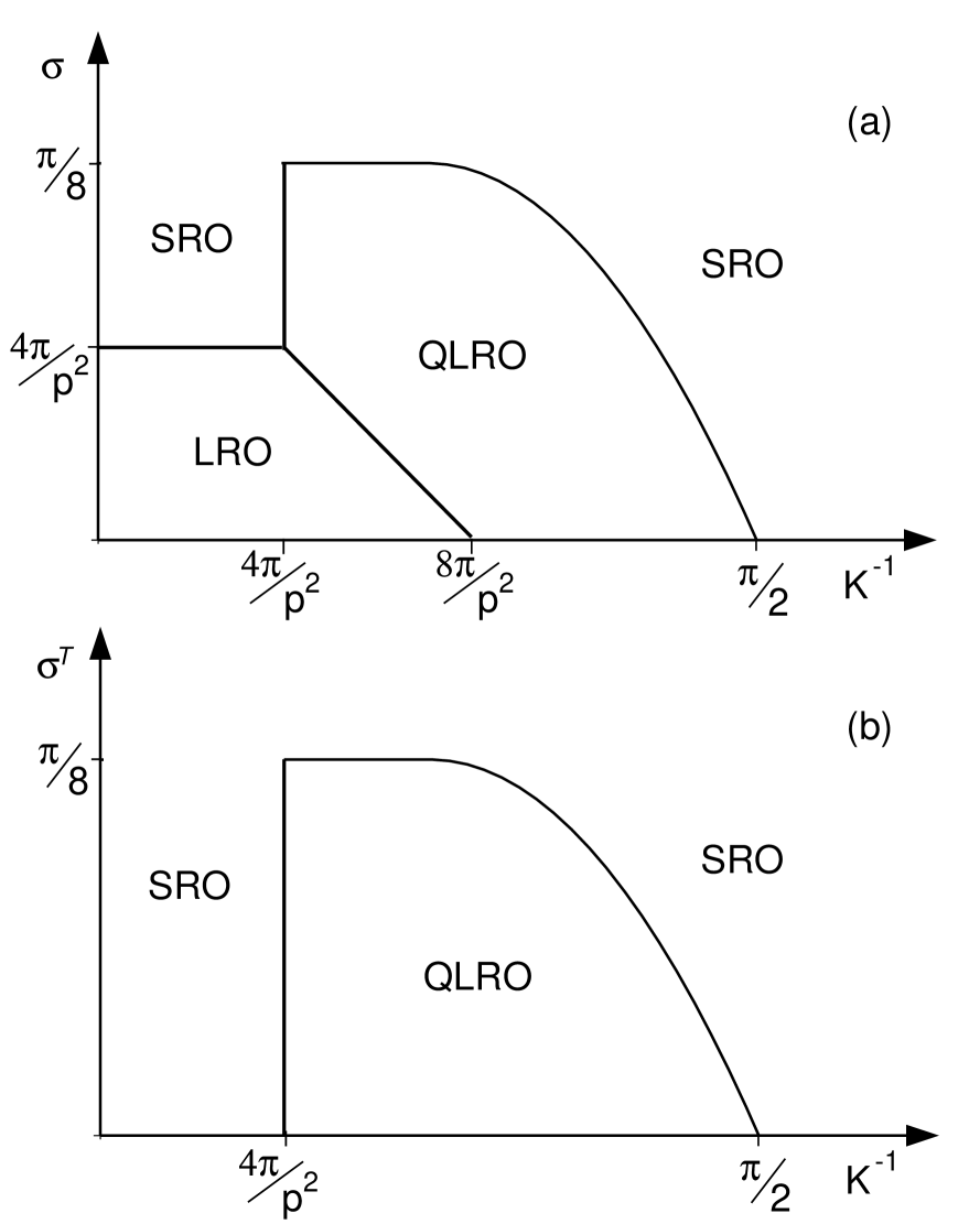
FIG. 1.: Generic phase diagrams (schematically) for the special cases of (a) uniform fields for $p>4$ and (b) random fields for $p>2\sqrt{2}$.

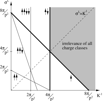
FIG. 2.: This diagram indicates the location of the lines on the low-temperature side of which various charges classes become relevant according to the scaling (52). In the shaded area all charges are irrelevant. In the whole parameter plane the most relevant charge class is either $\uparrow$ (on the high-temperature side of the dashed line at $K^{-1}=\sigma^{L}$) or $\uparrow\downarrow$ (on the low-temperature side of the dashed line).

FIG. 3.: Nonreentrant phase diagram in the absence of fields according to Refs. [19, 20, 21, 22, 23] and as it is reproduced by the flow equations (III E).

FIG. 4.: Phase diagram in the absence of vortices. The transition lines between the phases LRO, QLRO, and QSRO depend only weakly on small fields $H_{0}\ll 1$. The transition between LRO and QSRO is almost horizontal for weak fields.

FIG. 5.: Phase diagram for the model with $\sigma^{L}=\sigma^{T}=\sigma$ and uniform fields. It is obtained from a numerical integration of the flow equations (III E) for two different values of $H_{0}$ and $\gamma=1.6$.

REFERENCES

- [1] M. Rubinstein, B. Shraiman and D.R. Nelson, Phys. Rev. B27, 1800 (1983).
- [2] E. Granato and J.M. Kosterlitz, Phys. Rev. B33, 6533 (1986); Phys. Rev. Lett.62, 823 (1989).
- [3] B. Horovitz and A. Golub, Phys. Rev. B55, 14 499 (1997); (E) 57, 656 (1998).
- [4] J. Toner and D.P. DiVincenzo, Phys. Rev. B41, 632 (1990).
- [5] T. Nattermann, I. Lyuksyutov, and M. Schwartz, Europhys. Lett. 16, 253 (1991).
- [6] T. Hwa and D.S. Fisher, Phys. Rev. Lett.72, 2466 (1994).
- [7] D.R. Nelson, Phys. Rev. B 27, 2902 (1983).
- [8] C. Carraro and D.R. Nelson, cond-mat/9607184.
- [9] D. Carpentier and P. Le Doussal, cond-mat/9712227.
- [10] J.M. Kosterlitz and D.J. Thouless, J. Phys. C 6, 1181 (1973).
- [11] J.M. Kosterlitz, J. Phys. C 7, 1046 (1974).
- [12] V.L. Berezinskii, Zh. Eksp. Teor. Fiz. 61, 1155 (1971) [Sov. Phys. JETP. 34, 610 (1972)].
- [13] J.V. José, L.P. Kadanoff, S. Kirkpatrick and D. Nelson, Phys. Rev. B16, 1217 (1977); (E) 17, 1477 (1978).
- [14] For a scaling analysis of the relevance of fields, see also: V.L. Pokrovski and G.V. Uimin, Phys. Lett. A 45. 467 (1973); Zh. Eksp. Teor. Fiz. 65, 1691 (1973) [Sov. Phys. JETP 38, 847 (1974)].
- [15] A. Houghton, R.D. Kenway, and S.C. Ying, Phys. Rev. B23, 298 (1981).
- [16] J.L. Cardy and S. Ostlund, Phys. Rev. B25, 6899 (1982).
- [17] For an explicit discussion of the generation of random bond disorder by random fields and its effect on the spin correlation see also Refs. [35, 36, 37].
- [18] M. Paczuski and M. Kardar, Phys. Rev. B43, 8331 (1991).
- [19] T. Nattermann, S. Scheidl, S.E. Korshunov, and M.S. Li, J. Phys. I France 5, 565 (1995).
- [20] M.-C. Cha and H.A. Fertig, Phys. Rev. Lett.74, 4867 (1995).
- [21] S.E. Korshunov and T. Nattermann, Phys. Rev. B53, 2746 (1996).
- [22] S. Scheidl, Phys. Rev. B55, 457 (1997).
- [23] L.H. Tang, Phys. Rev. B54, 3350 (1996).
- [24] S.E. Korshunov, Phys. Rev. B48, 1124 (1993).
- [25] C. Mudry and X.-G. Wen, cond-mat/9712146.
- [26] J.M. Kosterlitz and M.V. Simkin, Phys. Rev. Lett.79, 1098 (1997).
- [27] J. Maucourt and D.R. Grempel, Phys. Rev. B56, 2572 (1997).
- [28] J. Villain, J. Phys. (France) 36, 581 (1975).
- [29] represents the constant added to the logarithm in Eq. (4.13) of Ref. [13].
- [30] S.F. Edwards and P.W. Anderson, J. Phys. F 5, 965 (1975).
- [31] A.P. Young, Phys. Rev. B19, 1855 (1979).
- [32] becomes the usual vortex fugacity and represents negligible higher orders. The agreement with the corrected flow equations Eq. (5.17) of Ref. [13] is given if one omits the exponential factors, which we understand as attempt to integrate the initial values for the fugacities.
- [33] The agreement is given if one replaces the factor multiplies the factor 4 in Eq. (3.7) of Ref. [16] by an additional factor [see dictionary (C1)].
- [34] However, there are nontrivial discrepancies in the second-order contributions to the flow equations (22) of Ref. [3].
- [35] Y.Y. Goldschmidt and A. Houghton, Nucl. Phys. B 210, 155 (1982).
- [36] J. Villain and and J.F. Fernandez, Z. Phys. B 54, 139 (1984).
- [37] Y.Y. Goldschmidt and B. Schaub, Nucl. Phys. B 251, 77 (1985).
- [38] D. Carpentier and P. Le Doussal, Phys. Rev. B55, 12 128 (1997).
- [39] S. Scheidl, Phys. Rev. Lett.75, 4760 (1995).
- [40] M.P.A. Fisher, T.A. Tokuyasu, and A.P. Young, Phys. Rev. Lett.66, 2931 (1991); M. Cieplak, J.R. Banavar, and A. Khurana, J. Phys. A 24, L145 (1991); H.S. Bokil and A.P. Young, Phys. Rev. Lett.74, 3021 (1995); R.A. Hyman, M. Wallin, M.P.A. Fisher, S.M. Girvin, and A.P. Young, Phys. Rev. B51, 15304 (1995).
- [41] R.M. Bowley and A.D. Armour, J. Low Temp. Phys. 107, 225 (1997).
- [42] P. Stahl, Diploma Thesis, Universität zu Köln (1997), cond-mat/9710344.
- [43] For further details, see: M. Lehnen, Diploma Thesis, Universität zu Köln (1997) (unpublished).