Vortex mediated microwave absorption in superclean layered superconductors.

Abstract

In the superclean case the spectrum of vortex core excitations in the presence of disorder is not random but consists of two series of equally-spaced levels.[1] The I-V characteristics of such superconductors displays many interesting phenomena. A series of resonances is predicted at frequencies commensurate with the spacing of the vortex excitations. These resonances reveal an even-odd anomaly. In the presence of one weak impurity the excitation levels can approach each other and almost cross. Absorption at low frequencies is identified with the resonances arising in this case. The results of such microscopic theory coincide up to the order of magnitude with both the theory employing kinetic equation[2] and the experiment.[3] The non-linear effects associated with Zener transitions in such crossings are studied. These phenomena can be used as a probe of vortex core excitations.

I Introduction

High-$T_{c}$ superconductors (HTSC) in normal state have many anomalous properties, differing them from normal metals. For example, the relaxation time depends on temperature according to the law $\tau^{-1}\approx T/2$ (assuming $\hbar=k_{\rm B}=1$). It is quite interesting if these properties remain anomalous below the transition, when superconductivity hinders studying them. Vortex cores retain a lot of information about the normal state. However, even in the BCS model the properties of vortex cores in superclean superconductors at low temperatures are studied insufficiently. The purpose of this work is to fill this gap.

It is believed that the dissipation in the mixed state of type II superconductors is associated with the low lying excitations arising inside the vortex cores, while they are dragged through the sample by the Lorentz forces [2]. Studying dissipation can therefore shine some light at both the spectrum and the relaxation mechanism of these excitations.

Although the excitation spectrum was calculated long ago[4], experimentalists approached the possibility of its observation only recently. [3, 5] To this end the excitation level spacing $\omega_{0}$ has to significantly exceed the broadening of levels due to various relaxation mechanisms $1/\tau$. This superclean case $\omega_{0}\tau\gg 1$ became possible in Cu based high-$T_{c}$ superconductors, as due to a very short coherence length $\xi$, both $\omega_{0}\sim 1/m\xi^{2}$ is large and the amount of disorder in the vortex core, contributing to the level broadening, is small. It should be noted that the measurements in Refs. [3, 5] are done at microwave frequencies to avoid the effects associated with pinning.

The DC absorption in superclean superconductors has been studied theoretically in a number of papers. [1, 2, 6] Among them the most notable is Ref. [2], in which the excitations were treated in the quasiclassically employing the kinetic equation in the $\tau$- approximation. The result of Ref. [2] for s-wave superconductors is

$$\rho_{\rm xx}=\frac{B}{n_{s}\left|e\right|c}\frac{1}{\omega_{0}\tau}$$ (1)

It should be noted however that contemporary high-$T_{c}$ superconductors are extremely anisotropic. For this reason the excitations in vortices become quasi two-dimensional (2D). It is known that in 2D the kinetic equation describes the scattering on impurities poorly. This is because a particle has a large probability to return to the original position and scatter on the same impurity many times. Therefore this problem can be treated i.e. considering the transitions between discrete levels.

Such treatment was realized in Ref. [7]. They used the random matrix theory to describe the transitions between excitation levels. Therefore their theory is not applicable to the superclean case.

The effects associated with the discreteness of the excitation spectrum in the superclean case have been added to consideration in Refs. [1, 6]. According to these references the discreteness of levels makes the absorption non-ohmic. Ref. [6] considers the shake up created by a weak impurity passing through the vortex core using the Fermi golden rule. They identify a critical velocity below which the non-ohmic effects should become pronounced. It can be estimated as

$$v_{c}=\frac{\omega_{0}}{k_{\rm F}},$$ (2)

where $k_{\rm F}$ is the Fermi momentum. Indeed the impurity passing through the core at velocity $v$ can create transitions between states separated by $\Omega=v/\lambda_{\rm F}$, as $\lambda_{\rm F}$ is the characteristic spacial frequency of the wavefunctions of the excitations. In the case $\Omega\lesssim\omega_{0}$ no transitions can occur and the absorption is exponentially small. The authors of Ref. [1] argue that even if impurity is weak, as long as the Born parameter of the impurity $\theta\gg\lambda_{\rm F}/\xi$, due to the special form of the excitation wavefunctions, the levels inside the vortex always cross. These crossings occur in the so-called dissipative region, when impurity is at the distances $a\approx\xi\theta$ from the center of the vortex. Here the Born parameter $\theta\lesssim 1$. The excitations in this case occur due to Landau-Zener transitions happening in the level crossings. Due to this effect the absorption at $v<v_{c}$ is not exponentially small but is much larger than given by Eq. (1).

It should be emphasized that the calculations in Refs. [1, 2, 6] have been done for the DC case. The experiments in Refs. [3, 5] are done at microwave frequencies ($\omega\approx 1.4K$). The $AC$ absorption in the superclean case has been studied in Refs. [8], [9], and [10]. All these studies are done using the kinetic equation in the $\tau$-approximation. This paper is dedicated to the microscopic study of the AC absorption in the superclean case. We adopt the mechanism of absorption used in Refs. [1, 6], i. e. the motion of vortex relative to the impurities brings about transitions of the excitations to the higher energy levels.

We study the global diagram of absorption as a function of frequency and amplitude of the applied current. We find that if the energy relaxation time $\tau_{\varepsilon}$ is large, the region on the diagram where kinetic equation gives the correct order of magnitude of the result becomes small.

The outline of our paper is as follows. In Sec. II we review some basic facts from Ref. [1] about the vortex core excitations in the presence of impurities in superclean layered superconductors. It is easy to see that in the superclean case the number of impurities per vortex core per crystalline layer can be estimated as $N_{i}\sim 1/\omega_{0}\tau\theta^{2}$. If $\theta\approx 1$ then it is very improbable to have more than one impurity inside the core in one layer. Another simplification comes from the fact that if coupling between layers is small (open Fermi surface), the excitation spectrum in the presence of impurity can be calculated independently for every layer. For this reason Ref. [1] treats the excitations in the presence of impurity as belonging to one two-dimensional layer. As a result they obtain that in the presence of impurity the usually equidistant spectrum of excitations, pertinent to the two-dimensional clean vortex core, ceases to be equidistant. However the spectrum remains to be strongly correlated. It is shown that the system of odd levels and the system of even ones separately continue to be equidistant with the level spacing $2\omega_{0}$ in each individual subsystem.

In Sec. IV be describe the resonances occurring in vortices under the influence of low amplitude, high frequency field. The amplitude of vortex motion $x_{0}$ is assumed to be much smaller than $\lambda_{\rm F}$, and frequency of external field $\omega$ is comparable or larger than $\omega_{0}$. We argue that the shape of resonant curves reveals an even-odd anomaly. If $\omega\approx 2n\omega_{0}$, where $n$ is integer, the transitions occur only within each individual subsystem of even or odd levels. In this case the resonance is very sharp, with the resonant curve determined by the remnant inelastic processes. If on the other hand $\omega\approx\left(2n+1\right)\omega_{0}$ the transitions between two subsystems of even and odd levels can occur. In this case the resonant frequency depends on the position of the impurity, and after averaging over this position the resonant curve of absorption becomes smeared.

In Sec. V we study the small amplitude low frequency absorption. In this case the transition can occur only in dissipative regions, where impurity makes even and odd levels cross. The result for ${\rm Re}\sigma_{xx}$ obtained in this case coincides with Eq. (1) in the order of magnitude. It is therefore purely ohmic.

The non-linear effects are associated with an increase of the amplitude $x_{0}$. They are of two types. The first is attributed to the saturation of energy absorption at long times [11]. It therefore effectively decreases the magnitude of energy dissipation. This non-linear effect can be neglected if $\omega\tau_{\epsilon}\ll 1$, where $\tau_{\epsilon}$ is the time of energy relaxation. In the latter case another non-linear effect becomes important. It arises due to Landau-Zener transitions between the crossing even and odd levels, as discussed in Ref. [1]. It therefore leads to an increase of absorption with respect to Eq. (1). In Sec. VI we present a phase diagram of various regimes of dissipation arising in this case.

Sec. VII is dedicated to our conclusions. We discuss the possible corrections to our results brought about by interlevel coupling, pinning, and d-wave order parameter. We compare our results to the existing experiment and discuss conditions at which resonances and non-linear effects can be observed.

II Vortex core excitations in the presence of an impurity.

In this Section we briefly review some facts about excitations inside the vortex core. They can be described by the Bogolyubov equations[4]:

$$\hat{\cal H}\left(\begin{array}[]{l}u\\ \\ v\end{array}\right)=E\left(\begin{array}[]{l}u\\ \\ v\end{array}\right),$$ (3)

where

$$\hat{\cal H}=\left(\begin{array}[]{ll}{\displaystyle\frac{\mathchoice{{\hbox{\boldmath$\displaystyle p$}}}{{\hbox{\boldmath$\textstyle p$}}}{{\hbox{\boldmath$\scriptstyle p$}}}{{\hbox{\boldmath$\scriptscriptstyle p$}}}^{2}}{2m}+V\left(\mathchoice{{\hbox{\boldmath$\displaystyle r$}}}{{\hbox{\boldmath$\textstyle r$}}}{{\hbox{\boldmath$\scriptstyle r$}}}{{\hbox{\boldmath$\scriptscriptstyle r$}}}-\mathchoice{{\hbox{\boldmath$\displaystyle a$}}}{{\hbox{\boldmath$\textstyle a$}}}{{\hbox{\boldmath$\scriptstyle a$}}}{{\hbox{\boldmath$\scriptscriptstyle a$}}}\right)-\mu;}&{\displaystyle\Delta\left(\mathchoice{{\hbox{\boldmath$\displaystyle r$}}}{{\hbox{\boldmath$\textstyle r$}}}{{\hbox{\boldmath$\scriptstyle r$}}}{{\hbox{\boldmath$\scriptscriptstyle r$}}}\right)}\\ \\ {\displaystyle\Delta\left(\mathchoice{{\hbox{\boldmath$\displaystyle r$}}}{{\hbox{\boldmath$\textstyle r$}}}{{\hbox{\boldmath$\scriptstyle r$}}}{{\hbox{\boldmath$\scriptscriptstyle r$}}}\right)^{*};}&{\displaystyle-\frac{\mathchoice{{\hbox{\boldmath$\displaystyle p$}}}{{\hbox{\boldmath$\textstyle p$}}}{{\hbox{\boldmath$\scriptstyle p$}}}{{\hbox{\boldmath$\scriptscriptstyle p$}}}^{2}}{2m}-V\left(\mathchoice{{\hbox{\boldmath$\displaystyle r$}}}{{\hbox{\boldmath$\textstyle r$}}}{{\hbox{\boldmath$\scriptstyle r$}}}{{\hbox{\boldmath$\scriptscriptstyle r$}}}-\mathchoice{{\hbox{\boldmath$\displaystyle a$}}}{{\hbox{\boldmath$\textstyle a$}}}{{\hbox{\boldmath$\scriptstyle a$}}}{{\hbox{\boldmath$\scriptscriptstyle a$}}}\right)+\mu}\end{array}\right).$$ (4)

Here $\Delta\left(\mathchoice{{\hbox{\boldmath$\displaystyle r$}}}{{\hbox{\boldmath$\textstyle r$}}}{{\hbox{\boldmath$\scriptstyle r$}}}{{\hbox{\boldmath$\scriptscriptstyle r$}}}\right)$, $\mu$, $V\left(r\right)$, and $\textstyle a$ are the order parameter, the chemical potential, the impurity potential, and the position of the impurity respectively. As it is mentioned in the introduction, in the superclean case we can consider no more than one impurity per vortex, per layer. We will assume that the magnetic field is weak ($B\ll H_{\rm C2}$) and therefore can be neglected in Eq. (4). We will also assume the s-wave order parameter to have the form

$$\Delta\left(\mathchoice{{\hbox{\boldmath$\displaystyle r$}}}{{\hbox{\boldmath$\textstyle r$}}}{{\hbox{\boldmath$\scriptstyle r$}}}{{\hbox{\boldmath$\scriptscriptstyle r$}}}\right)=\Delta\left(r\right)e^{i\phi},$$ (5)

where $r$ and $\phi$ are the polar coordinates.

The low energy excitation spectrum without impurity is well known: [4]

$$E^{0}_{n}=-\omega_{0}\left(n-\frac{1}{2}\right),$$ (6)

where

$$\begin{array}[]{l}{\displaystyle\omega_{0}=\frac{\displaystyle\int_{0}^{\infty}\frac{\Delta\left(r\right)dr}{r}e^{-2K\left(r\right)}}{\displaystyle k_{\rm F}\int_{0}^{\infty}dre^{-2K\left(r\right)}},}\\ \\ {\displaystyle K\left(r\right)=\frac{1}{v_{\rm F}}\int_{0}^{r}dr^{\prime}\Delta\left(r^{\prime}\right)},\\ \\ {\displaystyle n=0,\pm 1,\pm 2\ldots}.\end{array}$$ (7)

The corresponding wavefunctions are given by

$$\left(\begin{array}[]{l}u_{n}\\ \\ v_{n}\end{array}\right)=Ce^{-K\left(r\right)}\left(\begin{array}[]{l}{\displaystyle e^{in\phi}J_{n}\left(k_{\rm F}r\right)}\\ \\ {\displaystyle-e^{i\left(n-1\right)\phi}J_{n-1}\left(k_{\rm F}r\right)}\end{array}\right),$$ (8)

with $J_{n}\left(x\right)$ being the Bessel function and $C$ being the normalization constant:

$$C^{2}=\frac{k_{\rm F}}{\displaystyle 4\int_{0}^{\infty}e^{-2K\left(r\right)dr}}.$$ (9)

If Kramer-Pesch effect takes place[12] at low temperatures ($T\ll T_{c}$) $\Delta(r)\approx\Delta(r=\infty)\equiv\Delta_{\infty},~{}r\gg\xi\frac{T}{T_{c}}$. Therefore, $K(r)$ is given by

$$K(r)=\frac{\Delta_{\infty}}{v_{\rm F}}r,~{}~{}r\gg\xi\frac{T}{T_{c}}.$$ (10)

Consequently

$$\begin{array}[]{l}{\displaystyle C^{2}=\frac{m\Delta_{\infty}}{2}}\\ \\ {\displaystyle\omega_{0}=\frac{\Delta_{\infty}^{2}}{\varepsilon_{\rm F}}\ln\left(\frac{T_{c}}{T}\right)}\end{array}$$ (11)

The excitation spectrum in the presence of a short range impurity at point $\textstyle a$ has been obtained in Ref. [1]. The energy spectrum is given by the following equation

$$\cos\left(\frac{\pi E}{\omega_{0}}\right)=-\frac{\displaystyle 4\pi\omega_{0}I_{1}}{\displaystyle 4\omega_{0}^{2}+\pi^{2}\left|I\right|^{2}}$$ (12)

where

$$I=I_{2}+iI_{1}=\frac{2C^{2}}{\pi k_{\rm F}a}e^{-2K\left(a\right)}\tilde{V}\left(2k_{\rm F}\right)e^{2ik_{\rm F}a}$$ (13)

and $\tilde{V}\left(q\right)$ is the Fourier transform of the impurity potential. In the derivation of (12) it has been assumed that $a\gg k_{\rm F}^{-1}$.

Note that in the absence of impurity ($I_{1}=I=0$) the spectrum given by Eq. (12) is equidistant and coincides with Eq. (6). However, in the presence of impurity the spectrum ceases to be equidistant. This is illustrated in Fig.  1, where the energy levels are shown as functions of the distance of the impurity from the center of the vortex.

FIG. 1.: The excitation energy levels as functions of the distance of the impurity from the vortex center $a$. The parameters used are: $\lambda_{\rm F}/\xi=0.1$ and $\theta\Delta_{\infty}/\omega_{0}k_{\rm F}\xi=0.9$ [see explanation following Eq. (14) below]. Only the vicinity of the dissipative region is shown.

However, the spectrum remains strongly correlated. It is easy to see from Eq. (12) and from the Fig. 1 that it comprises two series of equidistant levels. The spacing within each series is $2\omega_{0}$, while with respect to each other they are shifted by a phase depending on the impurity.

Another feature of the spectrum evident from the Figure is that when the impurity is close to the center it bring about periodic anticrossings of the levels. The minimum distance between levels in such anticrossings $\delta E$, according to Ref. [1], has a minimum at point $a=a_{0}$ and is determined by the equation:

$$\begin{array}[]{l}{\displaystyle\delta E\approx\frac{d\left|I\right|}{da}\left|a-a_{0}\right|},\\ \\ {\displaystyle\left|I\left(a_{0}\right)\right|=\frac{2\omega_{0}}{\pi}}.\end{array}$$ (14)

Eq. (14) together with Eqs. (11) and (13) give

$$a_{0}=\frac{\theta\Delta_{\infty}}{k_{\rm F}\omega_{0}}=\frac{\pi\theta}{2\ln\left(T_{c}/T\right)}\xi.$$ (15)

Here $\theta=m\tilde{V}\left(2k_{\rm F}\right)$ is the Born parameter. The region of the vortex near $a=a_{0}$ is the region where levels approach each other very closely. For this reason Zener transitions are very probable there. Therefore it was called in Ref. [1] the dissipative region.

III Motion of the vortices

Below we recollect a few facts pertinent to the absorption by vortices. We consider the system of vortices in an alternating electric field oriented in the plane of the layers. The magnetic field $\textstyle B$ is perpendicular to the layers. If pinning is negligible the velocity of all of the vortices is the same. Let us denote it

$$\mathchoice{{\hbox{\boldmath$\displaystyle v$}}}{{\hbox{\boldmath$\textstyle v$}}}{{\hbox{\boldmath$\scriptstyle v$}}}{{\hbox{\boldmath$\scriptscriptstyle v$}}}\left(t\right)=\mathchoice{{\hbox{\boldmath$\displaystyle v$}}}{{\hbox{\boldmath$\textstyle v$}}}{{\hbox{\boldmath$\scriptstyle v$}}}{{\hbox{\boldmath$\scriptscriptstyle v$}}}\cos\left(\omega t\right).$$ (16)

Therefore the position of impurity relative to the vortex is given by

$$\mathchoice{{\hbox{\boldmath$\displaystyle a$}}}{{\hbox{\boldmath$\textstyle a$}}}{{\hbox{\boldmath$\scriptstyle a$}}}{{\hbox{\boldmath$\scriptscriptstyle a$}}}=\mathchoice{{\hbox{\boldmath$\displaystyle\bar{a}$}}}{{\hbox{\boldmath$\textstyle\bar{a}$}}}{{\hbox{\boldmath$\scriptstyle\bar{a}$}}}{{\hbox{\boldmath$\scriptscriptstyle\bar{a}$}}}+\mathchoice{{\hbox{\boldmath$\displaystyle x$}}}{{\hbox{\boldmath$\textstyle x$}}}{{\hbox{\boldmath$\scriptstyle x$}}}{{\hbox{\boldmath$\scriptscriptstyle x$}}}_{0}\sin\left(\omega t\right),$$ (17)

where $\mathchoice{{\hbox{\boldmath$\displaystyle x$}}}{{\hbox{\boldmath$\textstyle x$}}}{{\hbox{\boldmath$\scriptstyle x$}}}{{\hbox{\boldmath$\scriptscriptstyle x$}}}_{0}$ is the amplitude of vibrations related to the electric field by

$$x_{0}=\frac{v}{\omega}.$$ (18)

It is convenient to write the Schroedinger equation for the time-dependent hamiltonian $\hat{\cal H}=\hat{\cal H}\left(t\right)$ [see Eq. (4)] in the basis of eigenfunctions of this hamiltonian considering time a parameter. These eigenfunctions $\left|n\left(t\right)\right>$ and the corresponding eigenvalues $E_{n}\left(t\right)$ can be used to obtain the differential equation for the occupation of these states[13]

$$\dot{c}_{n}=\sum_{m\neq n}c_{m}\frac{\left<m\right|\frac{\partial\hat{\cal H}}{\partial t}\left|n\right>}{E_{m}\left(t\right)-E_{n}\left(t\right)}c_{m}e^{i\left[\phi_{m}\left(t\right)-\phi_{n}\left(t\right)\right]}.$$ (19)

Here $\phi_{n}=\int_{0}^{t}E\left(t^{\prime}\right)dt^{\prime}$.

In Sec. IV and V we will consider cases when $x_{0}\ll\lambda_{\rm F}$. The transition probability between levels $m$ and $n$ in this case can determined by the Fermi golden rule

$$\begin{array}[]{ll}{\displaystyle w_{m\rightarrow n}}&{\displaystyle=\frac{\pi}{2}\left|\left<m\right|\delta{\hat{\cal H}}\left|n\right>\right|^{2}}\\ \\ {}&{\displaystyle\times\delta\left[\omega-E_{n}\left(\bar{\mathchoice{{\hbox{\boldmath$\displaystyle a$}}}{{\hbox{\boldmath$\textstyle a$}}}{{\hbox{\boldmath$\scriptstyle a$}}}{{\hbox{\boldmath$\scriptscriptstyle a$}}}}\right)+E_{m}\left(\bar{\mathchoice{{\hbox{\boldmath$\displaystyle a$}}}{{\hbox{\boldmath$\textstyle a$}}}{{\hbox{\boldmath$\scriptstyle a$}}}{{\hbox{\boldmath$\scriptscriptstyle a$}}}}\right)\right].}\end{array}$$ (20)

Here the perturbation to the hamiltonian in the system of reference moving with the condensate

$$\delta{\hat{\cal H}}=\left(\begin{array}[]{ll}{\displaystyle\mathchoice{{\hbox{\boldmath$\displaystyle x$}}}{{\hbox{\boldmath$\textstyle x$}}}{{\hbox{\boldmath$\scriptstyle x$}}}{{\hbox{\boldmath$\scriptscriptstyle x$}}}_{0}\partial V/{\partial\mathchoice{{\hbox{\boldmath$\displaystyle r$}}}{{\hbox{\boldmath$\textstyle r$}}}{{\hbox{\boldmath$\scriptstyle r$}}}{{\hbox{\boldmath$\scriptscriptstyle r$}}}};}&{\displaystyle 0}\\ \\ {0;}&{\displaystyle-\mathchoice{{\hbox{\boldmath$\displaystyle x$}}}{{\hbox{\boldmath$\textstyle x$}}}{{\hbox{\boldmath$\scriptstyle x$}}}{{\hbox{\boldmath$\scriptscriptstyle x$}}}_{0}\partial V/{\partial\mathchoice{{\hbox{\boldmath$\displaystyle r$}}}{{\hbox{\boldmath$\textstyle r$}}}{{\hbox{\boldmath$\scriptstyle r$}}}{{\hbox{\boldmath$\scriptscriptstyle r$}}}};}\end{array}\right)$$ (21)

The energy absorption due to one impurity is given by

$$Q_{1}\left(\bar{\mathchoice{{\hbox{\boldmath$\displaystyle a$}}}{{\hbox{\boldmath$\textstyle a$}}}{{\hbox{\boldmath$\scriptstyle a$}}}{{\hbox{\boldmath$\scriptscriptstyle a$}}}}\right)=\omega\sum_{n,m}w_{m\rightarrow n}\left[f_{n}-f_{m}\right],$$ (22)

where $f_{n}=f\left(E_{n}\right)=\left[\exp\left(\frac{E_{n}-\mu}{T}\right)+1\right]^{-1}$ is the Fermi distribution function. The absorption averaged over many impurities and vortices is determined by

$$Q=n_{\rm i}n_{\rm v}\int d^{2}\bar{\mathchoice{{\hbox{\boldmath$\displaystyle a$}}}{{\hbox{\boldmath$\textstyle a$}}}{{\hbox{\boldmath$\scriptstyle a$}}}{{\hbox{\boldmath$\scriptscriptstyle a$}}}}Q_{1}\left(\bar{\mathchoice{{\hbox{\boldmath$\displaystyle a$}}}{{\hbox{\boldmath$\textstyle a$}}}{{\hbox{\boldmath$\scriptstyle a$}}}{{\hbox{\boldmath$\scriptscriptstyle a$}}}}\right).$$ (23)

Here $n_{\rm i}$ is the three-dimensional (3D) concentration of impurities, while $n_{\rm v}$ is the 2D concentration of vortex lines.

Let us now establish the connection between the electric field in the plane of the layers $\mathchoice{{\hbox{\boldmath$\displaystyle\cal{E}$}}}{{\hbox{\boldmath$\textstyle\cal{E}$}}}{{\hbox{\boldmath$\scriptstyle\cal{E}$}}}{{\hbox{\boldmath$\scriptscriptstyle\cal{E}$}}}(t)$ and the velocity of the vortices $\mathchoice{{\hbox{\boldmath$\displaystyle v$}}}{{\hbox{\boldmath$\textstyle v$}}}{{\hbox{\boldmath$\scriptstyle v$}}}{{\hbox{\boldmath$\scriptscriptstyle v$}}}(t)$. The AC electric field in a superconductor can be written as a sum of two terms:

$$\mathchoice{{\hbox{\boldmath$\displaystyle\cal{E}$}}}{{\hbox{\boldmath$\textstyle\cal{E}$}}}{{\hbox{\boldmath$\scriptstyle\cal{E}$}}}{{\hbox{\boldmath$\scriptscriptstyle\cal{E}$}}}=-\frac{1}{4\pi\lambda^{2}}\frac{d\mathchoice{{\hbox{\boldmath$\displaystyle j$}}}{{\hbox{\boldmath$\textstyle j$}}}{{\hbox{\boldmath$\scriptstyle j$}}}{{\hbox{\boldmath$\scriptscriptstyle j$}}}_{s}}{dt}-\mathchoice{{\hbox{\boldmath$\displaystyle v\times B$}}}{{\hbox{\boldmath$\textstyle v\times B$}}}{{\hbox{\boldmath$\scriptstyle v\times B$}}}{{\hbox{\boldmath$\scriptscriptstyle v\times B$}}}/c,$$ (24)

where $\lambda$ is the London penetration depth and $\mathchoice{{\hbox{\boldmath$\displaystyle j$}}}{{\hbox{\boldmath$\textstyle j$}}}{{\hbox{\boldmath$\scriptstyle j$}}}{{\hbox{\boldmath$\scriptscriptstyle j$}}}_{s}$ is the supercurrent. Here the first term is the London electric field in the inertial system of reference in which vortices are not moving. The other term arises due to the flux carried by the vortices with velocity $\textstyle v$.

Let us supplement this formula with the general equations for the electric field and dissipation:

$$\begin{array}[]{l}{\mathchoice{{\hbox{\boldmath$\displaystyle\cal{E}$}}}{{\hbox{\boldmath$\textstyle\cal{E}$}}}{{\hbox{\boldmath$\scriptstyle\cal{E}$}}}{{\hbox{\boldmath$\scriptscriptstyle\cal{E}$}}}=\mathchoice{{\hbox{\boldmath$\displaystyle\hat{\rho}j$}}}{{\hbox{\boldmath$\textstyle\hat{\rho}j$}}}{{\hbox{\boldmath$\scriptstyle\hat{\rho}j$}}}{{\hbox{\boldmath$\scriptscriptstyle\hat{\rho}j$}}},}\\ \\ {Q=\rm{Re}\rho_{\rm xx}\overline{j^{2}}},\end{array}$$ (25)

where the line denotes the time averaging. Further we consider the case of small temperatures ($T\ll T_{c}$), when the relative contribution to the current from normal electrons is exponentially small. Therefore we can assume $j\approx j_{s}$.

In the superclean case $\rm{Im}\rho_{xx}$ and $\rho_{xy}$ are weakly dependent on the density of impurities. Hence they can be fairly well approximated by the values for clean system. Another simplification appears if the spectrum of electrons is isotropic. Then $\mathchoice{{\hbox{\boldmath$\displaystyle j$}}}{{\hbox{\boldmath$\textstyle j$}}}{{\hbox{\boldmath$\scriptstyle j$}}}{{\hbox{\boldmath$\scriptscriptstyle j$}}}_{s}=en_{s}\mathchoice{{\hbox{\boldmath$\displaystyle v$}}}{{\hbox{\boldmath$\textstyle v$}}}{{\hbox{\boldmath$\scriptstyle v$}}}{{\hbox{\boldmath$\scriptscriptstyle v$}}}_{s}$ and $\lambda^{-2}=4\pi e^{2}n_{s}/mc^{2}$. Eq. (25) can then be rewritten as the equation of motion of the center of mass of the condensate:

$${m\dot{\mathchoice{{\hbox{\boldmath$\displaystyle v$}}}{{\hbox{\boldmath$\textstyle v$}}}{{\hbox{\boldmath$\scriptstyle v$}}}{{\hbox{\boldmath$\scriptscriptstyle v$}}}}_{s}=e\mathchoice{{\hbox{\boldmath$\displaystyle\cal{E}$}}}{{\hbox{\boldmath$\textstyle\cal{E}$}}}{{\hbox{\boldmath$\scriptstyle\cal{E}$}}}{{\hbox{\boldmath$\scriptscriptstyle\cal{E}$}}}+e\mathchoice{{\hbox{\boldmath$\displaystyle v$}}}{{\hbox{\boldmath$\textstyle v$}}}{{\hbox{\boldmath$\scriptstyle v$}}}{{\hbox{\boldmath$\scriptscriptstyle v$}}}_{s}\times\mathchoice{{\hbox{\boldmath$\displaystyle B$}}}{{\hbox{\boldmath$\textstyle B$}}}{{\hbox{\boldmath$\scriptstyle B$}}}{{\hbox{\boldmath$\scriptscriptstyle B$}}}/c-\eta\mathchoice{{\hbox{\boldmath$\displaystyle v$}}}{{\hbox{\boldmath$\textstyle v$}}}{{\hbox{\boldmath$\scriptstyle v$}}}{{\hbox{\boldmath$\scriptscriptstyle v$}}}_{s}}.$$ (26)

Here $\eta$ is the effective viscosity. Calculation of this viscosity as a function of frequency and velocity is the purpose of this work. Notice that it has both real and imaginary components. The real part can be calculated from the absorption:

$${Q(\omega)={\rm Re}\eta\overline{v_{s}^{2}}.}$$ (27)

The imaginary part is somewhat irrelevant due to the fact that it is compared to the London term [left-hand side of Eq. (26)]. At the same time ${\rm Im}\eta$ has to vanish in the absence of impurities as in the opposite case it would shift the position of the cyclotron resonance, violating the Kohn’s theorem[14]. Therefore in the superclean case it is small compared to the left-hand side of Eq. (26) and can be neglected.

Eq. (24) together with Eq. (26) result in the following equation for the vortex motion:

$$\mathchoice{{\hbox{\boldmath$\displaystyle v$}}}{{\hbox{\boldmath$\textstyle v$}}}{{\hbox{\boldmath$\scriptstyle v$}}}{{\hbox{\boldmath$\scriptscriptstyle v$}}}_{s}-\mathchoice{{\hbox{\boldmath$\displaystyle v$}}}{{\hbox{\boldmath$\textstyle v$}}}{{\hbox{\boldmath$\scriptstyle v$}}}{{\hbox{\boldmath$\scriptscriptstyle v$}}}=\mathchoice{{\hbox{\boldmath$\displaystyle\hat{z}$}}}{{\hbox{\boldmath$\textstyle\hat{z}$}}}{{\hbox{\boldmath$\scriptstyle\hat{z}$}}}{{\hbox{\boldmath$\scriptscriptstyle\hat{z}$}}}\times\mathchoice{{\hbox{\boldmath$\displaystyle v$}}}{{\hbox{\boldmath$\textstyle v$}}}{{\hbox{\boldmath$\scriptstyle v$}}}{{\hbox{\boldmath$\scriptscriptstyle v$}}}_{s}\eta/m\omega_{c}.$$ (28)

Here $\omega_{c}=|e|B/mc$ is the cyclotron frequency. In the superclean case the ratio $\eta/m\omega_{c}$ is proportional to the density of impurities. In the majority of cases considered below this quantity is small. For example the kinetic equation at zero frequency gives the following estimate for this quantity:

$$\eta/m\omega_{c}=1/\omega_{0}\tau\ll 1.$$ (29)

Our calculations discussed below confirm this result. Therefore for the superclean case it is plausible to assume that $\textstyle v$ is close to $\mathchoice{{\hbox{\boldmath$\displaystyle v$}}}{{\hbox{\boldmath$\textstyle v$}}}{{\hbox{\boldmath$\scriptstyle v$}}}{{\hbox{\boldmath$\scriptscriptstyle v$}}}_{s}$ [see Eq. (28)], i.e. the condensate and the vortices almost do not move with respect to each other.

Eq. (26) can also be used to obtain an expression for the resistivity tensor:

$$\begin{array}[]{l}{\displaystyle\rho_{\rm xx}=\frac{B}{n_{s}|e|c}\left(-i\frac{\omega}{\omega_{c}}+\frac{\eta}{m\omega_{c}}\right),}\\ \\ {\displaystyle\rho_{\rm xy}(\omega)=\frac{B}{n_{s}ec}.}\end{array}$$ (30)

The dissipative component of the conductivity tensor following from this expression is given by:

$${\rm Re}\sigma_{\rm xx}=\frac{n|e|c}{B}\frac{\gamma\omega_{c}^{2}\left(\omega^{2}+\omega_{c}^{2}+\omega_{c}^{2}\gamma^{2}\right)}{\left(\omega^{2}-\omega_{c}^{2}-\omega_{c}^{2}\gamma^{2}\right)^{2}+4\gamma^{2}\omega_{c}^{2}\omega^{2}},$$ (31)

where $\gamma={\rm Re}\eta/m\omega_{c}$ is small in the superclean case in accordance with Eq. (29). At small frequencies Eq. (31) can be seen to describe the cyclotron resonance. The cyclotron resonance in superconductors was observed experimentally in Ref. [15] and was described by Ref. [10] in the framework of the kinetic equation in the $\tau$-approximation. Note that the cyclotron resonance rendered by this expression is sharp if $\gamma\ll 1$ or exactly in the conditions of superclean case. Note also that as Eq. (31) is a consequence of quite general equation of motion of condensate (26). In the derivation of Eq. (31) we have neglected by the imaginary part of $\eta$ in comparison to $m\omega$. It is possible to do so because ${\rm Im}\eta$ has to vanish in the absence of impurities. In the opposite case it would shift the position of the cyclotron resonance, violating the Kohn’s theorem[14], as it was mentioned before.

Let us analize the influence of pinning on the motion of the condensate. We will ignore the dissipation for a moment. If pinning is present the pinning force has to be added to the total force acting on the condensate in Eq. (26):

$$\mathchoice{{\hbox{\boldmath$\displaystyle F$}}}{{\hbox{\boldmath$\textstyle F$}}}{{\hbox{\boldmath$\scriptstyle F$}}}{{\hbox{\boldmath$\scriptscriptstyle F$}}}_{p}=-i\alpha\mathchoice{{\hbox{\boldmath$\displaystyle v$}}}{{\hbox{\boldmath$\textstyle v$}}}{{\hbox{\boldmath$\scriptstyle v$}}}{{\hbox{\boldmath$\scriptscriptstyle v$}}}/\omega.$$ (32)

Here $i\mathchoice{{\hbox{\boldmath$\displaystyle v$}}}{{\hbox{\boldmath$\textstyle v$}}}{{\hbox{\boldmath$\scriptstyle v$}}}{{\hbox{\boldmath$\scriptscriptstyle v$}}}/\omega$ is the displacement of the vortex lattice (assuming it to be rigid), $\alpha$ is the pinning parameter, related to the critical current $j_{c}$ by

$$\alpha=\frac{Bj_{c}}{cn_{s}\xi}\equiv m\omega_{p}^{2}.$$ (33)

In the last expression we have introduced the pinning frequency $\omega_{p}$. This frequency can be related to the critical velocity $v_{p}\equiv j_{c}/n_{s}|e|$ and the cyclotron frequency by

$$\omega_{p}^{2}=\frac{v_{p}}{\xi}\omega_{c}.$$ (34)

Eqs. (24) and (26) give the following expression for the modified by pinning frequency of the cyclotron resonance:

$$\tilde{\omega}=\frac{\omega_{c}^{2}+\omega_{p}^{2}}{\omega_{c}}$$ (35)

In the limit $\omega_{p}\rightarrow 0$, $\tilde{\omega}\rightarrow\omega_{c}$. At a non-zero $\omega_{p}$ the cyclotron resonance occurs at a frequency larger then $\omega_{c}$ (Ref. [10]). At the same time the equation of vortex motion, Eq. (28)

$$\mathchoice{{\hbox{\boldmath$\displaystyle v$}}}{{\hbox{\boldmath$\textstyle v$}}}{{\hbox{\boldmath$\scriptstyle v$}}}{{\hbox{\boldmath$\scriptscriptstyle v$}}}_{s}-\mathchoice{{\hbox{\boldmath$\displaystyle v$}}}{{\hbox{\boldmath$\textstyle v$}}}{{\hbox{\boldmath$\scriptstyle v$}}}{{\hbox{\boldmath$\scriptscriptstyle v$}}}=i\mathchoice{{\hbox{\boldmath$\displaystyle\hat{z}$}}}{{\hbox{\boldmath$\textstyle\hat{z}$}}}{{\hbox{\boldmath$\scriptstyle\hat{z}$}}}{{\hbox{\boldmath$\scriptscriptstyle\hat{z}$}}}\times\mathchoice{{\hbox{\boldmath$\displaystyle v$}}}{{\hbox{\boldmath$\textstyle v$}}}{{\hbox{\boldmath$\scriptstyle v$}}}{{\hbox{\boldmath$\scriptscriptstyle v$}}}\omega_{p}^{2}/\omega\omega_{c}.$$ (36)

Therefore the pinning is important if $\omega\ll\omega_{p}^{2}/\omega_{c}$.

Pinning can be ignored at large frequencies ($\omega\gg\tilde{\omega}$) or if velocity is larger than $j_{c}/N_{s}|e|$. Then Eq. (31) gives

$${\rm Re}\sigma_{\rm xx}\approx{\rm Re}\rho_{\rm xx}\left(\frac{\omega_{c}}{\omega}\right)^{2}\left(\frac{n|e|c}{B}\right)^{2}$$ (37)

Using this expression one can relate the resonance structure arising in ${\rm Re}\rho_{\rm xx}$ near $\omega\approx\omega_{0}$ to that in ${\rm Re}\sigma_{\rm xx}$. This resonance is described in the next Section.

IV Resonances at high frequency and small amplitude.

In this Section we will assume the displacement of the vortex due to the driving field to be much smaller than the smallest scale at hand $\lambda_{\rm F}$. In this case to calculate absorption it is only natural to employ the Fermi golden rule. The absorption averaged over a large interval of $\omega$ in this linear response formalism is of the same order of magnitude as given by Eq. (1). However at the frequencies equal to multiples of $\omega_{0}$ resonances occur in the sample. The aim of this Section is to calculate the absorption near these resonances.

Eq. (20) emphasizes that at the conditions of resonance the energies of two states $E_{n}$ and $E_{m}$ should be close to the multiples of $\omega_{0}$. This implies that they should not be disturbed strongly from the values in the absence of impurity given by Eq. (6). Therefore near resonances the main contribution to the integral in Eq. (23) comes from the regions far from the center of the vortex $\theta\xi\sim a_{0}\ll\bar{a}$. In these regions one can treat the influence of impurity perturbatively. In the first order of the impurity potential we obtain the following expressions for the correction to the energy of excitation from Eq. (12)

$$\begin{array}[]{ll}{\Delta E_{n}}&{\equiv E_{n}-E_{0n}\approx(-1)^{n}I_{1}(\bar{a})}\end{array}$$ (38)

At these conditions the transition probability in the first non-vanishing order in the impurity potential can be determined taking as wavefunctions the states of the hamiltonial with no impurity [Eq. (8)]. Eq. (21) then gives

$$\left<m\right|\delta{\hat{\cal H}}\left|n\right>\approx 2k_{\rm F}x_{0}\cos\phi\left\{\begin{array}[]{ll}{I_{2}(\bar{a}),}&{{\rm even}~{}n+m,}\\ \\ {I_{1}(\bar{a}),}&{{\rm odd}~{}n+m.}\end{array}\right.$$ (39)

Here $\phi$ is the angle between $\textstyle\bar{a}$ and $\mathchoice{{\hbox{\boldmath$\displaystyle x$}}}{{\hbox{\boldmath$\textstyle x$}}}{{\hbox{\boldmath$\scriptstyle x$}}}{{\hbox{\boldmath$\scriptscriptstyle x$}}}_{0}$. The golden rule expression (20) can be readily rewritten as follows

$$\begin{array}[]{ll}{Q}&{\displaystyle=n_{\rm i}n_{\rm v}\frac{\pi\omega}{2}\int d\phi\bar{a}d\bar{a}\sum_{n,m}\left[f_{n}-f_{m}\right]}\\ \\ {}&{\displaystyle\left|\left<m\right|\delta{\hat{\cal H}}\left|n\right>\right|^{2}\delta\left[\Delta\omega-I_{1}\left\{(-1)^{n}-(-1)^{m}\right\}\right]},\end{array}$$ (40)

where $\Delta\omega=\omega-l\omega_{0}<\omega_{0}/2$, with $l$ being integer, is the deviation of the frequency from the resonance, and index of the matrix element should be chosen in accordance with Eq. (39).

Looking at the $\delta$-function in this expression one immediately sees that the answer should be quite different for $\omega$ close to even and odd multiples of $\omega_{0}$ (for even and odd $l$). Indeed if $l$ is even the resonant $\delta$-function reduces to $\delta(\Delta\omega)$. Therefore the condition of resonance is the same at any position of impurity relative to the center of vortex. Hence $\delta(\Delta\omega)$ appears as a factor in front of the expression for absorption. Therefore the resonances are very sharp in this case.

In the opposite case, when $l$ is odd, the resonances can occur even if $\Delta\omega$ is not zero, due to the shift of energy levels by the impurity. Thus for odd $l$ the resonances are broadened by the presence of impurity. This difference between even and odd $l$ is a consequence of the mentioned in Sec. II property of the spectrum. The series of odd and even levels are shifted with respect to each other by the impurity, preserving equal spacing of $2\omega_{0}$ within each series. Thus the resonances at even frequencies occur within each series of levels and are sharp, while the perturbation at odd frequencies mixes even and odd levels, making resonance broader. Below we study these two cases separately.

A) Odd $\omega/\omega_{0}$.

Eq. (40) for this case can be rewritten as follows

$$\begin{array}[]{ll}{Q}&{\displaystyle=n_{\rm i}n_{\rm v}\frac{2\pi^{2}\omega^{2}}{\omega_{0}}k_{\rm F}^{2}x_{0}^{2}\int\bar{a}d\bar{a}\left(\frac{\Delta\omega}{2}\right)^{2}}\\ \\ {}&{\displaystyle\times\delta\left[\Delta\omega-2\left|I(\bar{a})\right|\sin\left(2k_{\rm F}\bar{a}\right)\right].}\end{array}$$ (41)

The resonances in the integrand of the last expression occur very frequently (once in $\lambda_{\rm F}/4$). One can average contribution from these resonances over much larger intervals to obtain an integral over a slowly varying integrand:

$$\begin{array}[]{ll}{Q}&{\displaystyle=n_{\rm i}n_{\rm v}\frac{\pi\omega^{2}}{2\omega_{0}}k_{\rm F}^{2}x_{0}^{2}\Delta\omega^{2}}\\ \\ {}&{\displaystyle\times\int\frac{\bar{a}d\bar{a}}{\sqrt{\left[2\left|I\left(\bar{a}\right)\right|\right]^{2}-\Delta\omega^{2}}}.}\end{array}$$ (42)

The integral can be evaluated by changing the variable of integration from $\bar{a}$ to $\left|I\right|$. They are related by Eq. (13). The function $a\left(\left|I\right|\right)$ can be found asymptotically in two limiting cases

$$a\left(\left|I\right|\right)=\left\{\begin{array}[]{ll}{\displaystyle\frac{2C^{2}\theta}{\pi k_{\rm F}|I|m},}&{\displaystyle|I|\gg\theta\omega_{0}}\\ \\ {\displaystyle\frac{v_{\rm F}}{2\Delta_{\infty}}\ln\left(\frac{\theta\omega_{0}}{|I|}\right),}&{\displaystyle|I|\ll\theta\omega_{0}}.\end{array}\right.$$ (43)

Here

$$\theta\equiv m\tilde{V}\left(2k_{\rm F}\right)\ll 1$$ (44)

is the Born parameter of the impurity. Calculating the absorption in these limiting cases one obtains

$$Q=n_{\rm i}n_{\rm v}v^{2}\frac{2C^{4}\theta^{2}}{m^{2}\omega_{0}\Delta\omega},$$ (45)

for $\theta\omega_{0}\ll\Delta\omega\ll\omega_{0}$ and

$$Q=n_{\rm i}n_{\rm v}v^{2}\frac{\pi^{2}\varepsilon_{\rm F}\Delta\omega}{2\Delta_{\infty}^{2}\omega_{0}}\ln\left(\frac{\theta\omega_{0}}{\Delta\omega}\right),$$ (46)

for $\Delta\omega\ll\theta\omega_{0}$. It is convenient to express this answer in the units of absorption obtained from the kinetic equation. Assume that $\tau$ is determined by scattering on short range impurities:

$$\tau^{-1}=2\pi n_{\rm i}\nu\left|\tilde{V}\left(2k_{\rm F}\right)\right|^{2},$$ (47)

with $\nu=m/\pi$ being 2D density of states in the layers Then from Eq. (1) one obtains

$$Q_{\rm K}=\frac{B}{2n_{s}|e|c}\frac{j^{2}}{\omega_{0}\tau}=n_{\rm i}n_{\rm v}v^{2}\theta^{2}\frac{\varepsilon_{\rm F}}{\omega_{0}}.$$ (48)

To simplify our consideration we will accept the Kramer-Pesch ansatz, expressed by Eqs. (10) and (11), after what we obtain

$$\frac{Q}{Q_{\rm K}}=\displaystyle\frac{1}{\displaystyle 2\ln\left(\frac{T_{c}}{T}\right)}\frac{\omega_{0}}{\Delta\omega},$$ (49)

for $\theta\omega_{0}\ll\Delta\omega\ll\omega_{0}$ and

$$\frac{Q}{Q_{\rm K}}=\frac{\pi^{2}}{8}\ln\left(\frac{T_{c}}{T}\right)\frac{\Delta\omega}{\theta^{2}\omega_{0}}\ln\left(\frac{\theta\omega_{0}}{\Delta\omega}\right),$$ (50)

for $\Delta\omega\ll\theta\omega_{0}$.

It can be noticed from these equations that when the frequency approaches the resonance the absorption first increases in accordance with Eq. (49) and then decreases according to Eq. (50). The former expression therefore describes resonance near $\omega_{0}$, while the latter describes the antiresonance. The numerical evaluation of Eq. (42) shows that the absorption reaches its maximum of ${\rm max}(0.2/\theta;0.6)$ at point $\Delta\omega\approx 0.5\theta\omega_{0}$. If $\theta>0.3$ the resonant part is not very well pronounced. On the other hand the antiresonace at $\Delta\omega\lesssim 0.5\theta\omega_{0}$ exists independently of the value of the Born parameter. An antiresonant behavior has been described earlier in Ref. [10]. The width of the antiresonance obtained in this reference is $1/\tau$. We obtain for the width of the antiresonance $\Delta\omega\approx 0.5\theta\omega_{0}$. The discrepancy is the consequence of the mentioned failure of the $\tau$-approximation in (quasi)two dimensions.

Another perturbation causing the resonance could be due to the inertial forces. This perturbation is important because it exists even in the cores with no impurities. The corresponding correction to the hamiltonian, similarly to (21), is

$$\delta\hat{\cal H}_{\rm Inert}=\left(\begin{array}[]{ll}{\displaystyle\mathchoice{{\hbox{\boldmath$\displaystyle\hat{p}$}}}{{\hbox{\boldmath$\textstyle\hat{p}$}}}{{\hbox{\boldmath$\scriptstyle\hat{p}$}}}{{\hbox{\boldmath$\scriptscriptstyle\hat{p}$}}}\mathchoice{{\hbox{\boldmath$\displaystyle v$}}}{{\hbox{\boldmath$\textstyle v$}}}{{\hbox{\boldmath$\scriptstyle v$}}}{{\hbox{\boldmath$\scriptscriptstyle v$}}}_{s};}&{\displaystyle\mathchoice{{\hbox{\boldmath$\displaystyle x$}}}{{\hbox{\boldmath$\textstyle x$}}}{{\hbox{\boldmath$\scriptstyle x$}}}{{\hbox{\boldmath$\scriptscriptstyle x$}}}_{0}\nabla\Delta}\\ \\ {\displaystyle\mathchoice{{\hbox{\boldmath$\displaystyle x$}}}{{\hbox{\boldmath$\textstyle x$}}}{{\hbox{\boldmath$\scriptstyle x$}}}{{\hbox{\boldmath$\scriptscriptstyle x$}}}_{0}\nabla\Delta^{*};}&{\displaystyle\mathchoice{{\hbox{\boldmath$\displaystyle\hat{p}$}}}{{\hbox{\boldmath$\textstyle\hat{p}$}}}{{\hbox{\boldmath$\scriptstyle\hat{p}$}}}{{\hbox{\boldmath$\scriptscriptstyle\hat{p}$}}}\mathchoice{{\hbox{\boldmath$\displaystyle v$}}}{{\hbox{\boldmath$\textstyle v$}}}{{\hbox{\boldmath$\scriptstyle v$}}}{{\hbox{\boldmath$\scriptscriptstyle v$}}}_{s}}\end{array}\right).$$ (51)

Here the diagonal terms represent the Doppler shift of the energy of the quaziparticles caused by the condensate moving with velocity $\mathchoice{{\hbox{\boldmath$\displaystyle v$}}}{{\hbox{\boldmath$\textstyle v$}}}{{\hbox{\boldmath$\scriptstyle v$}}}{{\hbox{\boldmath$\scriptscriptstyle v$}}}_{s}$ (Ref. [9]), while the off-diagonal terms are associated with the motion of vortex itself.[8] The matrix element of (51) calculated between the pure states relevant to the neighborhood of the resonance can be rewritten as follows:

$$\left<m\right|\delta\hat{\cal H}_{\rm Inert}\left|n\right>=\left<m\right|\mathchoice{{\hbox{\boldmath$\displaystyle\hat{p}$}}}{{\hbox{\boldmath$\textstyle\hat{p}$}}}{{\hbox{\boldmath$\scriptstyle\hat{p}$}}}{{\hbox{\boldmath$\scriptscriptstyle\hat{p}$}}}\left(\mathchoice{{\hbox{\boldmath$\displaystyle v$}}}{{\hbox{\boldmath$\textstyle v$}}}{{\hbox{\boldmath$\scriptstyle v$}}}{{\hbox{\boldmath$\scriptscriptstyle v$}}}_{s}-\mathchoice{{\hbox{\boldmath$\displaystyle v$}}}{{\hbox{\boldmath$\textstyle v$}}}{{\hbox{\boldmath$\scriptstyle v$}}}{{\hbox{\boldmath$\scriptscriptstyle v$}}}\right)\sigma_{0}\left|n\right>.$$ (52)

Here $\sigma_{0}$ is the unit Pauli matrix. In this equation we used the identity:

$$\left<m\right|\sigma_{1}\mathchoice{{\hbox{\boldmath$\displaystyle x$}}}{{\hbox{\boldmath$\textstyle x$}}}{{\hbox{\boldmath$\scriptstyle x$}}}{{\hbox{\boldmath$\scriptscriptstyle x$}}}_{0}\nabla\Delta\left|n\right>=\left<m\right|[\nabla;\hat{H}]\left|n\right>=\left<m\right|\mathchoice{{\hbox{\boldmath$\displaystyle\hat{p}$}}}{{\hbox{\boldmath$\textstyle\hat{p}$}}}{{\hbox{\boldmath$\scriptstyle\hat{p}$}}}{{\hbox{\boldmath$\scriptscriptstyle\hat{p}$}}}\mathchoice{{\hbox{\boldmath$\displaystyle v$}}}{{\hbox{\boldmath$\textstyle v$}}}{{\hbox{\boldmath$\scriptstyle v$}}}{{\hbox{\boldmath$\scriptscriptstyle v$}}}\sigma_{0}\left|n\right>.$$ (53)

The absorption due to this perturbation is given by:

$$Q_{\rm Inert}=n_{v}n_{s}\frac{\omega_{0}}{4\tau_{\varepsilon}}\frac{\left(v-v_{s}\right)^{2}}{\Delta\omega^{2}+\tau_{\varepsilon}^{-2}},$$ (54)

where $v-v_{s}$ is given by either Eq. (28) or by Eq. (36). In case if pinning is negligible $\mathchoice{{\hbox{\boldmath$\displaystyle v$}}}{{\hbox{\boldmath$\textstyle v$}}}{{\hbox{\boldmath$\scriptstyle v$}}}{{\hbox{\boldmath$\scriptscriptstyle v$}}}_{s}$ is very close to $\textstyle v$, as it follows from Eq. (28). Taking an estimate for $\eta$ from Eq. (50) at $\Delta\omega\sim\tau_{\varepsilon}^{-1}$ the absorption due to the inertial forces can then be estimated as

$$Q_{\rm Inert}/Q_{\rm K}\sim 1/\omega_{0}^{2}\tau\tau_{\varepsilon}.$$ (55)

This is just a small correction to Eq. (50). The significant reduction of the absorption is a consequence of the Galellian invariance.

B) Even $\omega/\omega_{0}$.

In this case due to homogeneous broadening of the levels the $\delta$ function in Eq. (40) is replaced by the following expression:

$$\delta(\Delta\omega)=\frac{1}{\displaystyle\pi\tau_{\varepsilon}\left(\Delta\omega^{2}+\tau_{\varepsilon}^{-2}\right)}.$$ (56)

Eq. (13) gives the following result for the absorption

$$Q=n_{\rm i}n_{\rm v}\frac{4C^{4}\theta^{2}}{m^{2}\omega_{0}}\delta(\Delta\omega)\ln\left(\frac{1}{\theta}\right).$$ (57)

Using the Kramer-Pesch ansatz (10) and (11) one readily obtains

$$\frac{Q}{Q_{\rm K}}=\displaystyle\frac{\displaystyle\ln\left(\frac{1}{\theta}\right)}{\displaystyle\ln\left(\frac{T_{c}}{T}\right)}\delta(\Delta\omega)$$ (58)

Note, that the absorption averaged over frequency for $\omega>\omega_{0}$ is the same in both even and odd cases and equals to

$$\frac{\bar{Q}}{Q_{\rm K}}=\frac{1}{Q_{\rm K}\omega_{0}}\int_{(l-1/2)\omega_{0}}^{(l+1/2)\omega_{0}}d\omega Q(\omega)=\frac{\displaystyle\ln\left(\frac{1}{\theta}\right)}{\displaystyle\ln\left(\frac{T_{c}}{T}\right)}$$ (59)

V Small amplitude low frequency absorption.

At a frequency much smaller than $\omega_{0}$ absorption is only possible if the impurity makes two levels approach each other to a distance smaller than $\omega$. This is possible if impurity is situated within dissipative region described in Sec. (II). From Eq. (14) it follows that the condition $\delta E<\omega$, $\omega\rightarrow 0$ can be satisfied in a narrow region adjacent to $\bar{a}=a_{0}$. In this region odd and even levels periodically anticross, approaching each other to small distances.

When two levels are anomalously close all others can be ignored and the two-state system can be described by a hamiltonian

$$H=\left(\begin{array}[]{cc}{{\alpha}}&{{\delta}}\\ \\ {{\delta}}&{-{\alpha}}\end{array}\right),$$ (60)

where $\delta>0$ is a slowly varying function of the $\bar{a}$, while $\alpha$ changes rapidly and $\alpha=0$ at the point of level anticrossing. The eigenvalues of this two-level system are given by

$$\varepsilon=\pm\sqrt{\delta^{2}+\alpha^{2}}.$$ (61)

Comparing this equation with Eq. (12) in the neighborhood of the anticrossing one obtains the following expression for $\alpha$ and $\delta$

$$\begin{array}[]{l}{\displaystyle\delta=\frac{\delta E}{2}}\\ \\ {\displaystyle\alpha\approx I_{2}\approx\frac{2k_{\rm F}\delta a\omega_{0}}{\pi}},\end{array}$$ (62)

where $\delta E$ is given by Eq. (14) and $\delta a$ is the distance from the point of anticrossing. The eigenmodes of the hamiltonian are described by

$$a_{\pm}=\left(\begin{array}[]{l}{\displaystyle\sqrt{\frac{|\varepsilon|\pm\delta}{2|\varepsilon|}}}\\ \\ {\displaystyle\pm\sqrt{\frac{|\varepsilon|\mp\delta}{2|\varepsilon|}}}.\end{array}\right)$$ (63)

The upper and lower signs in this expression pertain to the states with positive and negative energy in Eq. (61). Now we can apply the golden rule expression for absorption (23) to this two-level system:

$$\begin{array}[]{ll}{Q}&{\displaystyle=n_{\rm i}n_{\rm v}\omega\int d\phi\bar{a}d\bar{a}\frac{\pi}{2}x_{0}^{2}\cos^{2}\phi}\\ \\ {}&{\displaystyle\times\left|\left<+\right|\frac{\partial H}{\partial a}\left|-\right>\right|^{2}\delta\left[\omega-2\varepsilon\left(\bar{a}\right)\right]},\end{array}$$ (64)

with

$$\left<+\right|\frac{\partial H}{\partial a}\left|-\right>=\frac{2}{\pi}k_{\rm F}\omega_{0}\frac{\delta}{|\varepsilon|}.$$ (65)

One can average over frequently occurring resonances in the integrand of Eq. (64) to obtain an integral over a slowly varying function

$$\begin{array}[]{ll}{Q}&{\displaystyle=2n_{\rm i}n_{\rm v}x_{0}^{2}k_{\rm F}^{2}\omega_{0}a_{0}}\\ \\ {}&{\displaystyle\times\int d\bar{a}\frac{\delta^{2}(\bar{a})}{\sqrt{\displaystyle\frac{\omega^{2}}{4}-\delta^{2}(\bar{a})}}}.\end{array}$$ (66)

Changing the variables of integration from $\bar{a}$ to $\delta$ using Eq. 14, i.e. using

$$d\bar{a}=4d\delta d\bar{a}/d|I|=2\pi a_{0}d\delta/\omega_{0},$$ (67)

we eventually obtain

$$\frac{Q}{Q_{\rm K}}=\frac{\pi^{2}}{\displaystyle 16\ln\left(\frac{T_{c}}{T}\right)}.$$ (68)

To obtain this answer we have employed the Kramer-Pesch ansatz (10) and (11).

Eq. (23) can also be evaluated for general $\omega$. The result reads

$$\begin{array}[]{ll}{\displaystyle\frac{Q}{Q_{\rm K}}}&{=\displaystyle\frac{\pi\omega_{0}}{\displaystyle 2\ln\left(\frac{T_{c}}{T}\right)\omega}\left[2{\rm floor}\left(\frac{\omega}{2\omega_{0}}\right)+1\right]}\\ \\ {}&{\displaystyle\times\left|\frac{\displaystyle\cos^{3}\left(\frac{\pi\omega}{2\omega_{0}}\right)-\cos\left(\frac{\pi\omega}{\omega_{0}}\right)}{\displaystyle\sin\left(\frac{\pi\omega}{\omega_{0}}\right)}\right|},\end{array}$$ (69)

where ${\rm floor}(x)$ is the maximum integer smaller or equal than $x$. Note that both asymptotics given by Eqs. (49) and (68) can be obtained from this expression in the limits $\omega\rightarrow 0$ and $\omega\rightarrow(2n+1)\omega_{0},~{}n=0,1,\ldots$ respectively. This result is shown in Fig. 2.

FIG. 2.: Absorption as a function of frequency determined by Eq. (69). At add frequencies only resonant behavior is shown. The sharp resonances at even frequencies [Eq. (58)] are shown by vertical lines. The non-zero limit$Q(\omega\rightarrow 0)$ is evaluated in this Section.

As it was mentioned in the previous Section, due to numerical reasons, the absorption at odd frequencies ($\omega_{0},3\omega_{0},\ldots$) does not raise above ${\rm max}(0.2/\theta;0.6)$. The resonances at odd frequencies can therefore be pronounced only if $\theta\lesssim 0.3$. We expect that in practice $\theta\lesssim 1$. Eq. (69) and Fig. 2 can therefore be understood only asymptotically in the limit $\theta\ll 1$.

VI Non-linear effects in the absorption

The non-linear effects in the absorption are interesting since in many cases they depend on the energy relaxation time of excitations. Therefore they can be used for studying this quantity. We attribute the non-linearities to two different phenomena. The first phenomenon is the saturation of absorption due to the redistribution of level occupations. It corresponds to the deviations from the golden rule expression (22). This leads to a decrease of the dissipative component of resistivity with respect to a linear response result. The second group of non-linear phenomena includes the effects associated with direct transitions between levels due to their anticrossings. They increase the absorption.

Consider the deviations from the golden rule expression first. In a two-level system the resonance with external field brings about the rotation of the population of the levels with Rabi frequency $\Omega_{\rm R}$. For the cases described in Sec. IV and V the Rabi frequency is given by:

$$\begin{array}[]{ll}{\Omega_{\rm R}}&{=\displaystyle\left|\left<m\right|\delta{\cal{H}}\left|n\right>\right|}\\ \\ {}&{\displaystyle\sim\omega_{0}\frac{x_{0}}{\lambda_{\rm F}}}.\end{array}$$ (70)

If the perturbation is applied during a time interval longer than $1/\Omega_{\rm R}$, the absorption saturates. In this case the system can absorb only if there are inelastic relaxation mechanisms present. If the corresponding relaxation time is $\tau_{\varepsilon}$, the energy $\omega$, corresponding to the external field frequency, is absorbed once in $\tau_{\varepsilon}$. This is in contrast to the golden rule expression, from which this time is seen to be $1/\Omega_{\rm R}$. To account for this this effect the absorption should be renormalized as follows

$$Q\rightarrow\frac{Q}{\sqrt{1+\Omega_{\rm R}^{2}\tau_{\varepsilon}^{2}}}.$$ (71)

The denominator in this expression is large if $v/v_{c}\gg\omega/\omega_{0}^{2}\tau_{\varepsilon}$. The absorption in this case is

$$Q\sim Q_{\rm K}\frac{v_{c}\omega}{v\omega_{0}^{2}\tau_{\varepsilon}}.$$ (72)

The non-linear effects are relatively abundant. To visualize them we draw a diagram in the space of parameters $v$ and $\omega$. This diagram is shown in Fig. 3. It displays the absorption measured in the units of $Q_{\rm K}$ given by Eq. (48).

The golden rule absorption considered in the previous two Sections is situated in sectors (a) and (b) of Fig. 3. The saturation of the golden rule expression becomes important on the line $v/v_{c}=\omega/\omega_{0}^{2}\tau_{\varepsilon}$. Eq. (72) determines the absorption in sector (d).

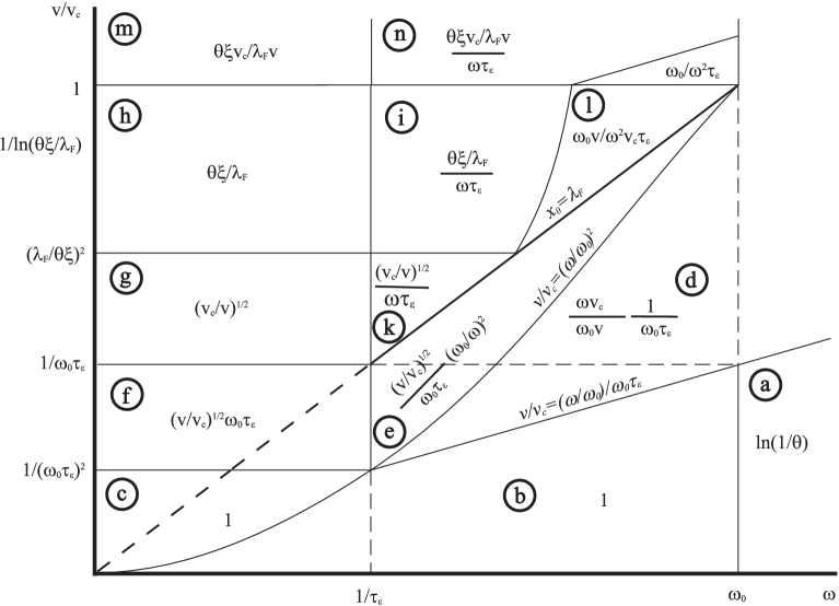
FIG. 3.: The diagram of absorption. The values of $Q/Q_{\rm K}$ are mapped for different regions in ($v/v_{c}$, $\omega$) plane. The equations for the boundaries between these region are made italic for convenience.

We now turn to the discussion of the influence of the Zener transitions between anticrossing levels. These transitions occur within the dissipative region, where some levels can be anomalously close. In this case the system of two almost degenerate states can be described by a two-level hamiltonian (60), and their energies are given by Eq. (61). The occupations of such a two-level system before the anticrossing $(p_{1},p_{2})$ and after the anticrossing $(p_{1}^{\prime},p_{2}^{\prime})$ are related as follows:[16]

$$\left(\begin{array}[]{l}{p_{1}^{\prime}}\\ {p_{2}^{\prime}}\end{array}\right)=\left(\begin{array}[]{ll}{1-W;}&{W}\\ {W;}&{1-W}\end{array}\right)\left(\begin{array}[]{l}{p_{1}}\\ {p_{2}}\end{array}\right).$$ (73)

The transition probability to the other level relevant for the absorption is

$$W=\exp\left(-\frac{\pi^{2}\delta E^{2}}{\displaystyle 4k_{\rm F}\omega_{0}v}\right).$$ (74)

Here $\delta E$ is the smallest distance between levels determined by Eq. (14).

Zener transitions can occur if $W\sim 1$. This determines the width of the dissipative region as well as the number of effectively working anticrossings there $N$. Indeed, if an impurity is situated in a ring of width $\lambda_{\rm F}N$ and radius $a_{0}\sim\theta\xi$ it can produce Zener transitions. We obtain from Eq. (14)

$$\delta E\sim\frac{d|I|}{da}\lambda_{\rm F}N\sim\frac{\omega_{0}}{\theta\xi}\lambda_{\rm F}N.$$ (75)

Then from Eq. (74) we have

$$N\sim\frac{\theta\xi}{\lambda_{\rm F}}\sqrt{\frac{v}{v_{c}}}.$$ (76)

One can distinguish two cases, depending on whether $N$ is large or small. If $N$ is large, an impurity passing through the dissipative region brings about many transitions. The opposite case $N\ll 1$ can be realized if velocity is small $v\ll v_{c}(\lambda_{\rm F}/\theta\xi)^{2}$. Below we first consider this latter case in some detail.

If $N\ll 1$, for a typical impurity Zener transitions are improbable. However if the Born parameter of the impurities has a little dispersion $\delta\theta=\sqrt{\left<\theta^{2}\right>-\left<\theta\right>^{2}}\neq 0$, the Zener transitions still can happen, yet on a very small fraction of impurities. Indeed, the current position of the level crossing $a$ is quantized in the units of $\lambda_{\rm F}/4$. The uncertainty of $a_{0}\sim\theta\xi$ is $\delta a_{0}\sim\delta\theta\xi$. Let us look at Eq. (14). If $\delta a_{0}>\lambda_{\rm F}/4$, $\delta E$ in this expression can accidentally become zero. This condition can also be rewritten as $\delta\theta>\lambda_{\rm F}/\xi\ll 1$. This assumption can therefore be realized even if the uncertainty of the Born parameter is small.

This can be reformulated in terms of an assumption about the distribution function of $\delta E$. In the case when $\delta\theta>\lambda_{\rm F}/\xi$ this distribution function $p(\delta E)$ has a non-zero limit when $\delta E$ goes to zero. In particular, taking Eq. (75) into account, we obtain

$$p(\delta E)=\frac{dN}{d[\delta E]}\sim\frac{\theta\xi}{\lambda_{\rm F}\omega_{0}}.$$ (77)

The expression for the total absorption Eq. (23) can be rewritten in this case as follows ($\bar{a}\sim\theta\xi$, $d\bar{a}\sim x_{0}$)

$$Q\sim n_{\rm i}n_{\rm v}\theta\xi x_{0}\int_{0}^{\infty}Q_{1}(\delta E)p(\delta E)d[\delta E],$$ (78)

where $Q_{1}(\delta E)$ is the absorption due to one impurity driving Zener transition on a couple of levels with the shortest separation $\delta E$. Our task from now on will be to estimate $Q_{1}$.

For the following discussion it is convenient to consider two cases $x_{0}\ll\lambda_{\rm F}$ and $x_{0}\gg\lambda_{\rm F}$ separately. In the first case an impurity can cause only one Zener transition per period, while in the second case there can be many.

A) $x_{0}\ll\lambda_{\rm F}$.

Consider an impurity at a distance less than $x_{0}$ from one of the anticrossings. Such an impurity can cause Zener transitions once in $\omega^{-1}$. The absorbed energy, however, depends on the relation between the characteristic time of Zener transition $\Delta t$ and the inelastic relaxation time $\tau_{\varepsilon}$. The former can be estimated as

$$\Delta t\sim\frac{\delta E}{\omega_{0}}\frac{\lambda_{\rm F}}{v}$$ (79)

and is the time during which two levels are at a distance of the order of $\delta E$. The absorption rate due to one such impurity can be estimated in three limiting cases as follows

$$Q_{1}\sim\left\{\begin{array}[]{ll}{\delta EW\omega,}&{\tau_{\varepsilon}\ll\Delta t}\\ \\ {\displaystyle\frac{v\tau_{\varepsilon}}{\lambda_{\rm F}}\omega_{0}W\omega,}&{\Delta t\ll\tau_{\varepsilon}\ll\omega^{-1}}\\ \\ {\displaystyle\frac{x_{0}}{\lambda_{\rm F}}\omega_{0}W\frac{1}{\tau_{\varepsilon}},}&{\Delta t\ll\omega^{-1}\ll\tau_{\varepsilon}}\end{array}\right.$$ (80)

As it has been mentioned above this is true if the impurity is at a distance smaller than $x_{0}$ from the anticrossing. In the opposite case the Zener transitions cannot occur and the absorption is negligible. Eqs. (78) and (80) then result in three limiting cases

$$Q\sim Q_{\rm K}\left\{\begin{array}[]{ll}{\displaystyle\sqrt{\frac{v}{v_{c}}}\omega_{0}\tau_{\varepsilon};}&{\displaystyle\omega\tau_{\varepsilon}\ll 1,~{}\frac{v}{v_{c}}\gg\frac{1}{\omega_{0}^{2}\tau_{\varepsilon}^{2}}}\\ \\ {1;}&{\displaystyle\omega\tau_{\varepsilon}\ll 1,~{}\frac{v}{v_{c}}\ll\frac{1}{\omega_{0}^{2}\tau_{\varepsilon}^{2}}}\\ \\ {\displaystyle\frac{\omega_{0}^{2}}{\omega^{2}}\frac{1}{\omega_{0}\tau_{\varepsilon}}\sqrt{\frac{v}{v_{c}}};}&{\displaystyle\omega\tau_{\varepsilon}\gg 1.}\end{array}\right.$$ (81)

These limiting cases correspond to the regions labeled (f), (c), and (e) ($\lambda_{\rm F}\gg x_{0}$) correspondingly in the diagram in Fig. 3.

Note that for this case the answer does not change when velocity passes across the value $v=v_{c}\lambda_{\rm F}^{2}/\theta^{2}\xi^{2}$ where $N\sim 1$. This is due to the fact that if $x_{0}\ll\lambda_{\rm F}$ even for the case $N\gg 1$ the moving impurity cannot produce more than one Zener transition per period $2\pi/\omega$. This happens not to be the case for $x_{0}\gg\lambda_{\rm F}$, when the boundary $v=v_{c}\lambda_{\rm F}^{2}/\theta^{2}\xi^{2}$ does exist.

B) $x_{0}\gg\lambda_{\rm F}$.

As it has been mentioned above for this case the division into small and large velocities is essential. We start from small velocities $v\ll v_{c}\lambda_{\rm F}^{2}/\theta^{2}\xi^{2}$, as in the experimental conditions[3] this is the region where the non-ohmic absorption can first be observed.

For small velocities a consideration analogous to Eq. (80) leads to

$$Q_{1}\sim\frac{1}{\omega\tau_{\varepsilon}}\tanh\left(\omega\tau_{\varepsilon}\right)\left\{\begin{array}[]{ll}{\delta EW\omega,}&{\tau_{\varepsilon}\ll\Delta t}\\ \\ {\displaystyle\frac{v\tau_{\varepsilon}}{\lambda_{\rm F}}\omega_{0}W\omega,}&{\Delta t\ll\tau_{\varepsilon}\ll\lambda_{\rm F}/v}\\ \\ {\displaystyle\frac{x_{0}}{\lambda_{\rm F}}\omega_{0}W\frac{1}{\tau_{\varepsilon}},}&{\Delta t\ll\lambda_{\rm F}/v\ll\tau_{\varepsilon}}\end{array}\right.$$ (82)

The factor $\tanh\left(\omega\tau_{\varepsilon}\right)/\omega\tau_{\varepsilon}$ accounts for the saturation of absorption when $\omega\gg\tau_{\varepsilon}^{-1}$. This is analogous to the saturation discussed in the Fermi golden rule case. This results in

$$Q\sim\frac{Q_{\rm K}}{\omega\tau_{\varepsilon}}\tanh\left(\omega\tau_{\varepsilon}\right)\left\{\begin{array}[]{ll}{\displaystyle\sqrt{\frac{v_{c}}{v}},}&{\displaystyle 1/\omega_{0}\tau_{\varepsilon}\ll v}\\ \\ {\displaystyle\sqrt{\frac{v}{v_{c}}},}&{\displaystyle 1/\omega_{0}^{2}\tau_{\varepsilon}^{2}v\ll 1/\omega_{0}\tau_{\varepsilon}}\\ \\ {\displaystyle 1,}&{v\ll 1/\omega_{0}^{2}\tau_{\varepsilon}^{2}.}\end{array}\right.$$ (83)

Note that for small frequencies $\omega\ll 1/\tau_{\varepsilon}$ we have reproduced two of the results from the previous case $x_{0}\ll\lambda_{\rm F}$, namely, sectors (f) and (c) of the diagram in Fig. 3. For this reason the line $x_{0}=\lambda_{\rm F}$ in this Figure is made dashed, as it does not divide physically different regions. We have also obtained a new result for sector (g).

Let us now discuss the case $N\gg 1$. If the amplitude of vortex motion $x_{0}$ exceeds $\lambda_{\rm F}N$, the impurity can cause $N$ Zener transitions per period of motion $2\pi/\omega$. This implies that the excitations can ballistically propagate up in energy to the hight $\omega_{0}N$ above the Fermi level. Therefore the power absorbed in one vortex can be written as follows

$$Q_{1}\sim\frac{1}{\tau_{\varepsilon}}\tanh\left(\omega\tau_{\varepsilon}\right)\omega_{0}N^{2}.$$ (84)

Hence, for the case $\lambda_{\rm F}N\ll x_{0}$ Eq. (23) results in ($\bar{a}\sim\theta\xi$, $d\bar{a}\sim x_{0}$)

$$\begin{array}[]{ll}{Q}&{\displaystyle\sim n_{\rm i}n_{\rm v}\theta\xi x_{0}Q_{1}}\\ \\ {}&{\displaystyle\sim Q_{\rm K}\left\{\begin{array}[]{ll}{\displaystyle\frac{\theta\xi}{\lambda_{\rm F}},}&{\displaystyle\omega\tau_{\varepsilon}\ll 1}\\ \\ {\displaystyle\frac{\theta\xi}{\lambda_{\rm F}\omega\tau_{\varepsilon}},}&{\displaystyle\omega\tau_{\varepsilon}\gg 1.}\end{array}\right.}\end{array}$$ (85)

These answers correspond to the sectors (h) and (i) in Fig. 3.

The equality $x_{0}=\lambda_{\rm F}N$ takes place on the line $v/v_{c}=(\omega\theta\xi/\omega_{0}\lambda_{\rm F})^{2}$. This line is the boundary between sectors (i) and (l) of the diagram. In sector (l) $x_{0}\ll\lambda_{\rm F}N$, and the maximum energy above the Fermi level that excitations can reach is $\omega_{0}x_{0}/\lambda_{\rm F}$. Therefore

$$Q_{1}\sim\frac{1}{\tau_{\varepsilon}}\tanh\left(\omega\tau_{\varepsilon}\right)\omega_{0}\left(\frac{x_{0}}{\lambda_{\rm F}}\right)^{2}.$$ (86)

Eq. (23) results in ($\bar{a}\sim\theta\xi$, $d\bar{a}\sim\lambda_{\rm F}N$)

$$\begin{array}[]{ll}{Q}&{\displaystyle\sim n_{\rm i}n_{\rm v}\theta\xi\lambda_{\rm F}NQ_{1}}\\ \\ {}&{\displaystyle\sim Q_{\rm K}\left\{\begin{array}[]{ll}{\displaystyle\sqrt{v/v_{c}},}&{\displaystyle\omega\tau_{\varepsilon}\ll 1}\\ \\ {\displaystyle\sqrt{v/v_{c}}/\omega\tau_{\varepsilon},}&{\displaystyle\omega\tau_{\varepsilon}\gg 1.}\end{array}\right.}\end{array}$$ (87)

These answers correspond to the sector (l) of Fig. 3.

Finally we would like to discuss the crossover between the regions (h), (i), and (l) and the non-ohmic regimes at high velocities in the sectors (m) and (n). When velocity exceeds the critical velocity $v_{c}$ the number of anticrossing is restricted by the size of the dissipative region. It is therefore

$$N\sim\frac{\theta\xi}{\lambda_{\rm F}}$$ (88)

Therefore the answers in sectors (m) and (n) can be obtained by renormalization those in sectors (h) and (i) by the factor $v_{c}/v$.

In the case of small frequencies $\omega\tau_{\varepsilon}\ll 1$ one can give the following interpolation formula for the absorption

$$\begin{array}[]{ll}{\displaystyle\frac{Q}{Q_{\rm K}}}&{\sim 1+\frac{\displaystyle 1}{\displaystyle\sqrt{v_{c}/v}/\omega_{0}\tau_{\varepsilon}+\sqrt{v/v_{c}}}}\\ \\ {}&{\displaystyle\frac{1}{\displaystyle\sqrt{v_{c}/v}/\omega_{0}\tau_{\varepsilon}+\theta\xi/\lambda_{\rm F}}\frac{1}{1+v/v_{c}}}\end{array}$$ (89)

The second term arises due to the Landau-Zener transitions on rare impurities, causing very small $\delta E$. Such impurities can therefore cause no more than one transition per period. The third term is associated with the cascade of Landau-Zener transitions. If $\omega_{0}\tau_{\varepsilon}<\theta\xi/\lambda_{\rm F}$, then the third term is larger than the second and sectors (g) and (k) in Fig. 3 do not exist.

VII Summary and Conclusions

In this work we have studied the influence of the discreteness of excitation levels on microwave absorption in superclean layered superconductors. At low amplitudes and low frequencies ($\omega\ll\omega_{0}$) the absorption coincides with the result of Ref. [2]. With increasing amplitude of vortex motion two non-linear effects are observed. In the case $\omega\tau_{\varepsilon}\gg 1$ an increase of the amplitude decreases the dissipative component of resistivity. This is due to the deviation of the occupation of the excitation levels from the Fermi distribution. In the opposite case $\omega\tau_{\varepsilon}\ll 1$ an increase of the amplitude brings about an increase of the dissipative component of resistivity due to Zener transitions. Therefore this effect can be used to measure the inelastic relaxation time.

In Sec. III we discuss the conditions at which the cyclotron resonance can be observed in superconductors. We find that the broadening of the resonant curve is $\omega_{c}/\omega_{0}\tau$. We conclude therefore that the cyclotron resonance is sharp if the condition of superclean case ($\omega_{0}\tau\gg 1$) is satisfied. This provides and independent way to measure this quantity. We also calculate the correction to the cyclotron frequency brought about by pinning.

For small amplitudes and large frequencies we obtain the series of antiresonances at the odd frequencies commensurate with the excitation level spacing [$(2n+1)\omega_{0}$, $n=0,~{}1,~{}2,~{}\ldots$], and the series of resonances at even frequencies commensurate with the level spacing [$2n\omega_{0}$]. Therefore the resonant behavior of the vortex cores in superclean superconductors reveals an even - odd anomaly. The existence of antiresonances at odd frequencies is associated with the retraction of the effectively working near the resonance impurity from the vortex to the distances $a\gg\xi$. There it creates very small matrix element of transition between vortex states. On the other hand at even frequencies the effectively working near the resonance impurity resides inside the vortex core ($a\lesssim\xi$).

Let us discuss the assumptions that we have made. We assumed the temperature to be sufficiently small. First, it has to be much smaller than $T_{c}$, so that the relevant excitations are given by Caroli - de Gennes - Matrison theory [4]. Second, $\tau_{\varepsilon}(T)$ should be large enough to satisfy the condition of the superclean case $\omega_{0}\tau_{\varepsilon}\gg 1$.

We also adopted the model of disorder consisting of strong short-range impurities with the Born parameter satisfying the condition $\theta\gg(\omega_{0}\tau)^{-1/2}$. At this condition there is no more than one impurity per vortex core per layer. In the opposite case of white noise disorder potential the excitation levels can be shown to be broadened by $\sqrt{\omega_{0}/\tau}$. This is analogous to the case of Landau level broadening by the white noise disorder considered in Ref. [17]. In this case we expect the absorption due to impurities at low frequencies ($\omega\ll\omega_{0}$) to be exponentially small. [18, 19]

We have considered 2D case assuming that tunneling between layers is small. In the presence of such tunneling the excitation levels with no impurities are broadened into band. The width of the band is of the order of $\delta\omega_{0}\sim\omega_{0}\epsilon$, where $\epsilon\ll 1$ is the anisotropy parameter. However, in the presence of impurity one level can leave the band and become discrete. The virtual transition to the other layers produce only small correction to the energy of this level and to our results. This correction can be accounted for by the renormalization of the impurity potential. However the antiresonances at $(2n+1)\omega_{0}$ and resonances at $2n\omega_{0}$ should be smeared in the presence of anisotropy. The finite homogeneous broadening of levels $\tau^{-1}_{\varepsilon}$ should also add some broadening to the (anti)resonances. We therefore conclude that the (anti)resonances should be broadened by ${\rm min}(\delta\omega_{0},~{}\tau^{-1}_{\varepsilon})$.

We disregarded pinning of the vortex lattice by the impurities in our consideration. It is possible to do so if the pinning does not affect motion of the lattice. This happens when $\omega_{p}^{2}<\omega\omega_{c}$, where $\omega_{p}$ is the characteristic pinning frequency introduced in Section III [Eq. (35)]. Pinning can also be neglected if the current significantly exceeds the critical current.

We have assumed the s-wave pairing mechanism in our treatment. In practice the superclean case can be realized in high-$T_{c}$ and organic superconductors. It is accepted to think that these materials have a d-wave coupling mechanism. Therefore it is important to study the absorption in d-wave superclean superconductors. This study has been done by Kopnin and Volovik [9] in the framework of kinetic equation in the $\tau$-approximation. We expect however that the differences between the results of kinetic equation and the microscopic approach studied in this work persist in the d-wave superconductors. Therefore we assume that some qualitative results obtained in our paper are applicable to these materials also. This matter requires a further study.

One of the known to us experiments on superclean samples is described in Refs. [3]. This paper reports a large $\omega_{0}\tau\approx 14$ observed in 90K single-crystal YBCO sample. This quantity weakly depends on temperature below 17K. Therefore we expect that at the conditions of weak temperature dependence scattering on impurities provides the main mechanism of absorption.

As it follows from our results the study of the frequency dependence and/or non-linear effects of absorption it is possible to determine the inelastic scattering time $\tau_{\varepsilon}$ even if it is much larger then the elastic one. Knowledge of $\tau_{\varepsilon}$ is important for understanding of the peculiarities of high-$T_{c}$ superconductors.[20, 21]

VIII Acknowledgements

The authors would like to express gratitude to Yu. M. Galperin, V. B. Geshkenbein, and B. I. Shklovskii for helpful discussions. A. K. was supported by NSF grant DMR-9616880, A. L. by NSF grant DMR-9812340.

REFERENCES

• [1] A. I. Larkin and Yu. N. Ovchinnikov, Phys. Rev. B57, 5457 (1997) [see also preprint/cond-mat 9708202 (1997)].
• [2] N. B. Kopnin and V. E. Kravtsov, JETP Lett. 23, 578 (1976); Sov. Phys. JETP 44, 861 (1986); Yu. M. Gal’perin and E. B. Sonin, Sov. Phys. Solid State 18, 1768 (1976); N. B. Kopnin and A. V. Lopatin, Phys. Rev. B51, 15291 (1995).
• [3] Y. Matsuda, N. P. Ong, J. M. Harris, J. B. Peterson, and Y. F. Yan, Phys. Rev. B49, 4380 (1994).
• [4] P. G. de Gennes, Superconductivity of Metals and Alloys, (Addison-Wesley Publishing Co., 1989).
• [5] J. M. Harris, Y. F. Yan, O. K. C. Tsui, Y. Matsuda, and N. P. Ong, Phys. Rev. Lett.73, 1711 (1994).
• [6] F. Guinea, Yu. Pogorelov, Phys. Rev. Lett.74, 462 (1995).
• [7] M. V. Feigel’man, and M. A. Skvortsov, Phys. Rev. Lett.78, 2640 (1997).
• [8] N. V. Kopnin, JETP Lett., 27, 391 (1978).
• [9] N. B. Kopnin, G. E. Volovik, Phys. Rev. Lett., 79, 1377 (1997).
• [10] Th. C. Hsu, Phys. Rev. B52, 9178 (1995); Physica C 213, 305 (1993).
• [11] M. Wilkinson and E. J. Austin, Phys. Rev. A46, 64 (1992).
• [12] L. Kramer and W. Pesch, Z. Physik 269, 59-64 (1974).
• [13] V. I. Kogan and V. M. Galitskiy, Problems in quantum mechanics, (Englewood Cliffs, N.J., Prentice-Hall, 1963).
• [14] W. Kohn, Phys. Rev. 123, 1242 (1961).
• [15] K. Kirrai, E. Choi, F. Dunmore, S. Liu, X. Ying, Qi Li, T. Venkatesan, H. D. Drew, Qi Li, and D. B. Fenner, Phys. Rev. Lett.69, 355 (1992); see also K. Kirrai et al., Phys. Rev. Lett.69, 152 (1992)
• [16] L. D. Landau and E. M. Lifshitz, Quantum Mechanics, (Reed Educational and Professional Publishing, 1996).
• [17] T. Ando, A. B. Fowler, and F. Stern, Reviews of Modern Physics, 54, 437 (1982).
• [18] T. Ando, Journ. of Phys. Soc. of Jap., 38, 989 (1975).
• [19] M. M. Fogler and B. I. Shklovskii, preprint cond-mat/9801165 (1998).
• [20] P. W. Anderson, Physica C 185-189, 11 (1991).
• [21] L. B. Ioffe, A. J. Millis, preprint cond-mat/9801092.