Kinetics of Nanopore Transport

Abstract

A nonlinear kinetic exclusion model is used to study osmosis and pressure driven flows through nearly single file pores such as antibiotic channels, aquaporins, zeolites and nanotubules. Two possible maxima in the steady state flux as a function of pore-solvent affinity are found. For small driving forces, the linear macroscopic osmotic and hydraulic permeabilities $P_{os}$ and $L_{p}$, are defined in terms of microscopic kinetic parameters. The dependences of the flux on activation energies, pore length and radius, and driving forces are explored and Arrhenius temperature dependences derived. Reasonable values for the physical parameters used in the analyses yield transport rates consistent with experimental measurements. Experimental consequences and interpretations are examined, and a straightforward extension to osmosis through disordered pores is given.

NOMENCLATURE

$$\begin{array}[]{llll}a&\mbox{effective molecular diameter}&\alpha&\mbox{left entrance rate}\\ n_{T}&\mbox{total particle number density}&\beta&\mbox{right exit rate}\\ n_{s}&\mbox{solute number density}&\gamma&\mbox{left exit rate}\\ k_{B}T&\mbox{thermal energy}&\delta&\mbox{left entrance rate}\\ \ell&\mbox{section length}&\lambda_{MFP}&\mbox{particle mean free path}\\ r_{p}&\mbox{pore entrance radius}&p(q)&\mbox{internal right(left) hop rate}\\ v_{T}&\mbox{thermal velocity}&\xi&(\alpha,\beta,\gamma,\delta,p,q)\\ A_{p}&\mbox{effective pore entrance area}&\chi_{0}^{(L,R)}&\mbox{left(right) solvent mole fraction}\\ E_{\xi}&\mbox{effective activation energies}&\chi_{s}^{(L,R)}&\mbox{left(right) solute mole fraction}\\ J_{i}(t)&\mbox{flux between section}\,i\,\mbox{and}\,i+1\,(1/t)&\sigma_{i}&\mbox{site $i$ occupation (0,1)}\\ J_{i}&\mbox{time average flux}\,(1/t)&\tau_{\xi}&\mbox{molecular transit times}\,(\xi^{-1})\\ L=N\ell&\mbox{pore length}&\Delta\mu_{0}&\mbox{solvent chemical potential difference}\\ L_{p}&\mbox{hydraulic permeability}&\Delta P&\mbox{hydrostatic pressure difference}\\ N&\mbox{number of pore sections}&\Delta\Pi&\mbox{osmotic pressure difference}\\ P_{os}&\mbox{osmotic permeability}&\Gamma&\mbox{acoustic attenuation coefficient}\\ &&\mbox{X}&\mbox{dimensionless driving}\\ \end{array}$$ (1)

]

I Introduction

Transport through microscopic pores is vital to many biological and industrial processes[1, 2, 3]. One phenomenon involving flow through microscopic channels is osmosis. Ubiquitous in biological functions such as cellular volume control, osmosis and reverse osmosis are also exploited in industrial processes such as solution concentration, filtration, and catalysis.

Living cells must transport nutrients, ions and water across their lipid membranes. Various biological structures and machinery, such as active transporters, cotransporters, antiporters, and simple channels or pores have evolved to perform these tasks [1, 2]. Of central importance in living organisms is the flow of water. Certain cells, such as nephrons, have a permeability to osmotically driven water transport too high to be explained by simple permeation through an oily lipid membrane bilayer. In addition to generic antibiotic pores such as gramicidin, pores which are apparently water specific (aquaporin-CHIP) have been identified [4]. By inserting aquaporins into their membranes, cells can in principle control overall osmotic permeabilities.

Mechanisms of fluid transport in confined geometries are also relevant in industrial applications, especially in separation processes. Both natural and manmade materials such as zeolites contain many molecular-sized, essentially single-file channels which can selectively absorb fluids. This size specificity can be exploited in separation of a mixture of linear and branched chain alkanes, where the zeolite acts like a sponge absorbing only the desired specie(s) [3]. Confining particles in zeolite pores can also serve to catalyze reactions [5, 6]. Therefore, there has been much research into fluid structure and transport within confined pores [7, 8, 9, 10, 11, 12, 13, 14, 15, 16].

Although the equilibrium properties of osmotic “pressure” are understood in terms of macroscopic forces [17] and statistical mechanics [18], nonequilibrium osmotic transport has been less well categorized. One approach uses macroscopic flow equations (such as the parabolic Poiseuillean fluid velocity profile through a pipe[19]); these, applied to structures of molecular dimensions lead to inaccurate prediction of membrane pore density, or pore radius, particularly in biological examples [2, 20]. Use of macroscopic parameters such as viscosity, or hydraulic flow, to microscopic transport has led to models that do not accurately describe most of the relevant microscopic physical processes [21, 22, 20] and many conflicting viewpoints [2]. A recent review of the historical controversies and misconceptions is given by Guell and Brenner [17], who present a clarifying macroscopic description of osmosis. Finkelstein [2] also mentions the many conceptual disagreements associated with osmosis and nonequilibrium thermodynamics, particularly when applied to water transport across biomembranes.

In this paper, we consider molecularly-sized pore that are nearly single-file. Many natural examples of pores are of molecular sizes. Zeolites typically have pores with radii $\sim 2-10\mbox{\AA}$ and length from a few nanometers to millimeters. Biological channels Integral membrane proteins that form channels in biological systems are difficult to prepare for X-ray crystallography, accurate dimensions of membrane water channels are not yet available. However, spanning cell membranes, they are $\sim 50\mbox{\AA}$ in length. Based on sequential analogies with antibiotic pores and electron cryocrystallography [26, 27] biopores such as the water transporting aquaporins are believed to have pore diameters $\sim 2-4\mbox{\AA}$. Thus, water movement inside these pores is statistically single-file, with “overtaking” rarely if at all occuring.

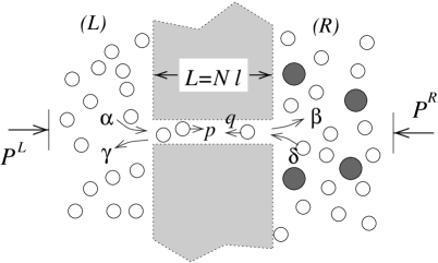
FIG. 1.: Schematic of osmosis and pressure driven flow through membrane pores. The reservoirs $(L)$ and $(R)$ are assumed infinite. The rates $\xi=(\alpha,\beta,\gamma,\delta,p,q)$ are conditional solvent entrance probabilities at the ends of the pore indicated (see text). For typical experiments, the membrane is impermeable to solute, $\Delta P=P^{R}-P^{L}$, $(L)$ contains pure solvent, and $J$ indicates the direction of solvent flux.

Using a symmetric exclusion model [28], thermodynamics, and simple kinetic theory, we formulate an approximate model for transport through nearly single-file pores [16] which can be solved exactly. Estimates of the microscopic kinetic parameters used allow the theory to be general enough to predict trends and to explore dependences on physical parameters such as pore geometry, microscopic interactions, and bulk fluid properties. Our model complements, although is more flexible than detailed numerical simulations. Microscopic motions derived from simulations can in principle be used to evaluate the system-dependent parameters used in this work, provided accurate force fields are known.

In the next Section, we review the usual linear phenomenological expressions used to describe osmosis or pressure driven flows through semipermeable membranes and identify all macroscopic variables. A one-dimensional symmetric exclusion model is then formulated for particle dynamics within a pore that connects two fluid reservoirs. The rate coefficients used are approximated using kinetic theory near thermodynamic equilibrium.

In the Results and Discussion, we explore the model as a function of reasonable parameters and present the mean flow rates in a series of plots. The macroscopic variables typically used are then related to the rate constants used in the microscopic theory. Nonlinearities and Arrenhius temperature dependences are also discussed. In the Conclusions, we summarize our results and introduce extensions to be studied in the following paper. The Appendix gives a simple result for pores with disordered interiors, or hopping rates.

II Membrane and Pore Transport Models

A Macroscopic Phenomenological Expressions

Here, we briefly review the macroscopic descriptions which hitherto have typically been used to model osmosis. The typical starting assumption is that the solvent flux is a function of the solvent chemical potential difference between two reservoirs (see Figure 1) that do not exchange solute. For two reservoirs with solvent at different equilibrium chemical potentials,

$$J=J(\Delta\mu)=\sum_{k=1}c_{k}(\Delta\mu_{0})^{k}=\sum_{k=1}d_{k}(-1)^{k}(\Delta\chi_{0})^{k},$$ (2)

where the last equality assumes $T^{L}=T^{R},\,P^{L}=P^{R}$, and $c_{k}$ and $d_{k}$ are expansion coefficients which may depend on external parameters such as temperature, pore-particle interactions, etc. They may also depend on the total solute concentration in the reservoirs. Equation (2) assumes linear response and expands $\Delta\mu$ in powers of solvent density (a virial expansion). The microscopic interactions are nearly identical for solvent in either reservoir (nearly all virial terms for the solvent chemical potential cancel) except for the infrequent encounters with solute in the solution $(R)$ side. To lowest order, the (low)solute concentration difference gives rise to the free energy difference which can be seen by using $\chi_{s}=1-\chi_{0}$, such that $J$ can be written in terms of solute mole fraction difference $\Delta\chi_{s}\equiv\chi_{s}^{R}-\chi_{s}^{L}$. A similar expansion in hydrostatic pressure gives van’t Hoff’s result that the solvent flow induced by an impermeable solute is thermodynamically balanced ($J=0$) by a hydrostatic pressure difference equal to $\Delta p=-\Delta\Pi=-k_{B}T(n_{T}^{R}\chi_{s}^{R}-n_{T}^{L}\chi_{s}^{L})\simeq-k_{B}Tn_{T}\Delta\chi_{s}$, where $n_{T}\simeq n_{T}^{L}\simeq n_{T}^{R}$ are the total particle number densities. Small currents between $(R)$ and $(L)$ are thus assumed (fairly accurately) to be linear $J\approx L_{p}(\Delta\Pi-\Delta p)$. Under isobaric conditions, and $\chi_{s}\ll 1$, osmotic flow is often represented by the osmotic permeability $P_{os}$ (also denoted $P_{f}$) where $J\simeq P_{os}(n_{s}^{R}-n_{s}^{L})$.

The constants of proportionality, $L_{p}$ and $P_{os}$ determine the rates of flow and have been the subject of considerable attention. Measurements of membrane permeabilities and the number of pores per area, can yield single pore conductivities. Conversely, the number of pores in a cell or vesicle can also be determined if single pore conductances can be accurately measured or modelled. Fully microscopic approaches, such as molecular dynamics (MD) simulations reveal detailed microscopic information on how fluids particles adsorb to the pore interior[23, 24]; however, the time scales readily achievable by MD ($\sim$ ns) cannot readily measure steady state flows through a long pore, or allow exploration of large parameter dependent flow regimes. To achieve channel flows in MD simulations, an external potential (such as gravity or external field) is often applied to every particle [25], to approximate a convective velocity. However, particles do not experience local “pondermotive” forces (as is the case in osmosis or pressure driven flows) in the absence of external electric or gravitational fields. In confined nearly 1D systems, such external forces may yield qualitatively different behavior (such as shocks in the particle density [28, 29]) from that expected in hydraulic or osmotic flow.

In the following, we analytically model particle dynamics through a single pore with the assumption that the reservoirs are in thermodynamic equilibrium, as was assumed in the expansion of $J$ (Eqn. (2)) about a thermodynamically defined $\Delta\mu_{0}$. We include sufficient microscopic detail within the pore, while carefully obeying all thermodynamic constraints in the connected reservoirs.

B One-dimensional Pore Exclusion Model

Our single-file model is similar to but more general than the one vacancy models of Hernandez [12] and Kohler [13]. The approach is fully microscopic, and does not rely on undefined hydrodynamic parameters (on these size scales) such as drag factors, viscosity, etc. Nonetheless, results from the microscopic theory can be associated and directly compared with those from experimental measurements. Consider the pore shown in Fig. 1 which depicts a single-file or nearly single-file pore. The main interactions that we include are the excluded particle (solvent) volumes within the pore; thus we adapt one-dimensional exclusion models [28, 16]. The pore is divided into $N$ sections labelled $i$, each of length $\ell$. The occupation variable $\sigma_{i}(t)$ defines whether pore section $i$ at time $t$ contains a particle ($\sigma_{i}(t)=1$) or is empty ($\sigma_{i}(t)=0$).

The discrete dynamics are defined by the follow rules: During any infinitesimal time interval $dt$, randomly chose a particle with label $0\leq i\leq N+1$, where $i=0,N+1$ corresponds to choosing the $(L),(R)$ reservoir. If $i=0$ (the left reservoir) is chosen during $dt$, and $\sigma_{1}(t)=0$, then we fill the first site $(\sigma_{1}=0)\rightarrow(\sigma_{1}(t+dt)=1)$ with probability $\alpha dt$. If $i=N+1$ (the right reservoir) and $\sigma_{N}(t)=0$, then we extract a particle from $(R)$ and set $\sigma_{N}(t+dt)=1$ with probability $\delta dt$. These steps allow injection of the end sites of the pore from the reservoirs if and only if the end sites are empty at time $t$. If a particle at $i=1$ is chosen, we empty it into the $(L)$ reservoir with probability $\gamma dt$, and if site $i=2$ is empty, we move the particle to the right with probability $pdt$. Similarly, if a particle at site $i=N$ is chosen, it moves into the $(R)$ reservoir with probability $\beta dt$, and if $\sigma_{N-1}(t)=0$, it moves to the left with probability $qdt$. If an interior site, $1<i<N$, is chosen, and $i+1\,(i-1)$ is empty, then we move the particle to the right(left) with probability $pdt\,(qdt)$ . The model assumes that $p$ and $q$ are constant along all the interior sites: Effects of site dependent $p=q$ are derived in Appendix A. All the moves are allowed only if the site to be entered is empty, except for the reservoirs $i=0,N+1$. After the a step is chosen and particles moved with the assigned probabilities, another particle is picked at random and the possible moves made. This algorithm is identical to a Monte Carlo simulation [30] except that spatial moves are coarse-grained to $\ell$ and the effective interaction energies (which determine the acceptance of moves) between particles are infinite (representing hard spheres) for a particle occupying the neighboring site, or zero if the site is empty. These kinetic steps can be summarized by the following instantaneous fluxes

$$J_{i}(t)=p\sigma_{i}(t)(1-\sigma_{i+1}(t))-q\sigma_{i+1}(t)(1-\sigma_{i}(t))\hskip 21.68121pt$$

$$\hskip 166.2212pt1<i<N-1$$

$$\begin{array}[]{lr}J_{(L)\rightarrow 1}(t)\equiv J_{0}(t)=\alpha(1-\sigma_{1}(t))-\gamma\sigma_{1}(t)&i=0\\[13.0pt] J_{N\rightarrow(R)}(t)\equiv J_{N}(t)=\beta\sigma_{N}(t)-\delta(1-\sigma_{N}(t))&i=N\end{array}$$ (3)

These dynamics implicitly include effective excluded volume interactions between solvent particles, which are strong in confined geometries such as 1D pores. However, we assume that solvent-solvent attractions within the pore are weak compared to solvent-pore particle attractions such that concerted cluster hops are rare. These processes can be be treated numerically [31] and is outside the scope of the present study.

To extract the steady-state currents and occupations, we take the time average $\langle\ldots\rangle$ of (3) to find

$$\begin{array}[]{l}\langle J_{i}(t)\rangle=p\langle\sigma_{i}(t)\rangle-q\langle\sigma_{i+1}(t)\rangle+(q-p)\langle\sigma_{i}(t)\sigma_{i+1}(t)\rangle\\[13.0pt] \langle J_{0}(t)\rangle=\alpha(1-\langle\sigma_{1}(t)\rangle)-\gamma\langle\sigma_{1}(t)\rangle\\[13.0pt] \langle J_{N}(t)\rangle=\beta\langle\sigma_{N}(t)\rangle-\delta(1-\langle\sigma_{N}(t)\rangle)\end{array}$$ (4)

Exact solutions to the steady state $\langle J(t)\rangle$ under certain parameter regimes and in the thermodynamic limit have been found using matrix algebra techniques [28, 29]. However, in osmosis and hydraulic pressure driven flows across symmetric pores, where the particles do not experience intrinsic or pondermotive forces, and have not developed collective stream velocities (c.f. Conclusions), $q=p$. That is, a particle is as likely to hop to the left or right if both sites to the left and right are unoccupied. The only “force” driving osmosis is the directionally asymmetric excluded volume along the length of the pore, which is ultimately determined by the entrance and exit rates at the boundaries $i=1,N$. Geometrically asymmetric pores would have $p\neq q$ and need to be treated numerically. The convective stream flow limit where also $p\neq q$, is discussed in the Conclusions. Many molecular dynamics simulations designed to study flow in narrow channels impose a microscopic pondermotive force with $p\neq q$ [25] (via a gravitational potential for example) in order to accelerate the flow. However, gravity and pressure forces, although macroscopically both derived from potentials, do not manifest themselves microscopically in the same way. When $q=p$ the higher order correlation $\langle\sigma_{i}(t)\sigma_{i+1}(t)\rangle$ vanishes in (4) and upon time averaging and invoking steady state particle conservation, $J_{i}=J_{i+1}=J_{i+2}=\ldots=J_{0}=J_{N}$, where we have dropped the $\langle\,\ldots\rangle$ notation. Since all the steady state currents across each interior section is identical, we can sum them up along the chain to obtain

$$J={p\over N-1}(\sigma_{1}-\sigma_{N})=J_{0}=J_{N}$$ (5)

Equations (5) give three equations for the three unknowns $J,\,\sigma_{1}$, and $\sigma_{N}$ which are found to be (with $\xi\equiv(\alpha,\beta,\gamma,\delta,p)$)

$$J(\xi,N)={p(\alpha\beta-\gamma\delta)\over(N-1)(\alpha+\gamma)(\beta+\delta)+p(\alpha+\beta+\gamma+\delta)}$$ (6)

and

$$\sigma_{1}={\alpha-J(\xi,N)\over\alpha+\gamma},\quad\sigma_{N}={\delta+J(\xi,N)\over\beta+\delta},$$ (7)

which determines $\sigma_{i}$,

$$\begin{array}[]{l}\displaystyle\sigma_{i}=\sigma_{1}-(i-1){J\over p}={\alpha\over\alpha+\beta}\\[13.0pt] \displaystyle\quad-{p(\alpha\beta-\gamma\delta)\over(\alpha+\beta)\left[(N-1)(\alpha+\gamma)(\beta+\delta)+p(\alpha+\beta+\gamma+\delta)\right]}\\[13.0pt] \displaystyle\quad\quad\quad-{(i-1)(\alpha\beta-\gamma\delta)\over(N-1)(\alpha+\gamma)(\beta+\delta)+p(\alpha+\beta+\gamma+\delta)}.\end{array}$$ (8)

For an infinitely thin membrane ($N=0$), the particles pass the mathematical surface based upon their reservoir kinematics alone and never interact with each other or the membrane interior while crossing the barrier. Overtaking of particles, when two adjacent, indistinguishable particles switch positions, does not contribute to the overall current. Therefore, the model above is also valid as long as each section $i$ is not too wide as to contain more than one particle at any time. Pore diameters of up to $2\sim 3$ times the particle diameters will on average preclude multiple occupancy.

C Parameter Relationships

The parameters $\xi\equiv(\alpha,\beta,\gamma,\delta,p)$ used in the above kinetic model are conditional probabilities and reveal the structure and microscopic mechanisms of osmosis and pressure driven flows. Here, we explicitly relate $\xi$ to macroscopic thermodynamic variables. Rather than find precise numerical values for $\xi$, we estimate them using reasonable physical models and extract their most sensitive dependences, thereby illustrating the qualitative features of osmosis and pressure driven flows through a pore.

The main assumption we make is that the entire system is under local thermodynamic equilibrium (LTE): Locally, particle velocities obey a Maxwellian distribution. This is justified since measurements of almost all microscopic systems give single pore osmotic transport rates of $J<10^{7}/$s. Typical pore diameters in aqueous solutions give mean free paths $\lambda_{MFP}\lesssim 5\mbox{\AA}$. Thus, ambient thermal velocities $v_{T}\simeq\sqrt{k_{B}T/m}\simeq 4\times 10^{4}$cm/s (where $m$ is the particle mass), give mean collision times of $\tau_{coll}\simeq\lambda_{MFP}/v_{T}\simeq 0.5\mbox{ps}\ll J^{-1}$. Therefore, particles within the pore equilibrate by suffering $O(10^{5})$ collisions while being transported from $(L)$ to $(R)$. This is sufficient for local thermodynamic equilibrium (LTE) to hold.

Figures 1(b) are schematics depicting the activation energies $E_{\xi}$ determined by microscopic membrane-solvent interactions. Although these are predominantly of an enthalpic nature, determined by instantaneous intermolecular potentials, a small entropic contribution may arise due to for example rotational averaging of nonspherically symmetric particles. We do not attempt to model in detail all the configurational dependences of particle trajectories, but rather assume the activation energies to be effective quantities, averaged over say, molecular rotations, internal vibrations, etc, which will not qualitatively affect the mean quantities we wish to study. $E_{p,q}$ are internal binding energies to the pore walls which must be overcome when particles hop from one section to another and can be thought of as effective interaction energies between pore and solvent. As mentioned, the model presented is valid provided solvent-solvent attraction within the pore $\ll E_{p}$. $E_{\beta,\gamma}$ and $E_{\alpha,\delta}$ are the effective energies of removing and injecting a particle. If we assume that there is no additional “constriction” at the pore ends, for a pore that repels particles relative to its interaction energies in the bulk reservoirs $(L)$ and $(R)$, $E_{\beta,\gamma}\simeq 0$ and $E_{\alpha,\delta}>0$ (Fig 2(a)). Similarly, as shown in Fig 2(b), an attractive pore will have $E_{\beta,\gamma}>0$ and $E_{\alpha,\delta}\simeq 0$. The physical origin of the energies such as $E_{\alpha}-E_{\gamma}$ defined in Figure 2(b) are most likely from hydrogen bonding interactions in aqueous systems. Transferring a water molecule from the polar, hydrogen bonding bulk environment into the pore region would require breaking hydrogen bonds ($\sim 5k_{B}T$ each) and forming van der Waals-type interactions with the pore interior.

FIG. 2.: Simplified pore-solvent interaction energy landscape for (a) repulsive and (b) attractive pores. The progression of the activation energies $E_{\xi}$ are indicated as pores are altered or conditions modified such that pore-solvent binding increases: $(a)\rightarrow(b)\rightarrow(c)$.

Additional activation energies at the entrance/exit sites would represent for example energetics of a possible intermediate state where hydrogen bonds are being broken, but attractive van der Waals interactions have not yet formed. For simplicity of notation, we assume these are small and neglect them. Inclusion of these boundary activation barriers will only shift the absolute values of $E_{\alpha},E_{\beta},E_{\gamma},E_{\delta}$ and will not qualitatively change our results.

The probabilities $\xi$ can be estimated by first passage time or transition state theory. The average time $\tau_{\xi}$ for a thermally agitated particle to climb over a barrier of height $E_{\xi}$ is given by

$$\tau_{\xi}\simeq\left[\xi_{0}\exp(-E_{\xi}/k_{B}T)\right]^{-1}$$ (9)

where $\xi_{0}$ is a thermal attempt frequency. The transition probabilities per time $\xi dt$ are thus given by $dt/\tau_{\xi}$. Upon choosing $dt\ll\tau_{\xi}$,

$$\xi\simeq\xi_{0}\exp(-E_{\xi}/k_{B}T).$$ (10)

The prefactors of $q=p$ and $\beta,\gamma$, are estimated by $p_{0},\beta_{0},\gamma_{0}\simeq v_{T}/\ell$. Although more sophisticated transition state theories exist, the thermal attempt frequencies are all on the order of 1ps^-1. The frequencies $\alpha_{0}$ and $\delta_{0}$ however, depend on the thermodynamic state of, and the particle numbers in the reservoirs $(L)$ and $(R)$ respectively, as well as the pore entrance areas. For example, for effusing dense gases, $\alpha_{0}=n_{T}^{L}v_{T}^{L}A_{p}^{L}/4$, proportional to the number density $n_{T}^{L}$ of particles able to enter, the thermal velocity $v^{L}_{T}$, and the available area $A^{L}_{p}$ for entrance. A completely analogous expression holds for $\delta_{0}$ with $(L)$ replaced by $(R)$. Although the $1/4$ factor is valid for gases, a qualitatively similar expression holds for dense liquids.

The microscopic pore area $A_{p}$ can be defined by $E_{\alpha,\delta}$. First consider $E_{\alpha}(\vec{r})$ to be a general interaction of pushing a particle perpendicularly through a membrane. When the particle is pushed through at a position $\vec{r}$ away from the pore (through a lipid layer for example), $E_{\alpha}(\vec{r})\simeq\infty$. When the trajectory runs through the center of an approximately circular pore entrance, $E_{\alpha}\equiv E_{\alpha}(\vec{r}=0)$. Therefore, we can define a pore radius $(A_{p}\simeq\pi r_{p}^{2})$ by demanding activation energies such that trajectories outside of $r_{p}$ are energetically rare. For example,

$$E_{\alpha}(r<r_{p})-E_{\alpha}(0)<\,\sim\!10k_{B}T.$$ (11)

Condition (11) simply contrains $r<r_{p}$ to be within a region where entrance is not impeded by “wall” interactions. Thus, $E_{\alpha}$ (and $E_{\delta}$) are the activation energies for a particle dragged through the approximate “centerline” of the pore. When more than one species occupies the reservoirs, but only one (the solvent) can enter the pore, the entrance rates will also be proportional to their mole fractions. For notational simplicity, we henceforth define $\alpha\equiv\alpha_{0}\chi_{0}^{L}\exp[-E_{\alpha}/k_{B}T]$ and $\delta\equiv\delta_{0}\chi_{0}^{R}\exp[-E_{\delta}/k_{B}T]$. Thus, $\alpha_{0}\propto A_{p}$ is now the rate prefactor for pure solvent entrance ($\chi_{0}=1$) at a reference number density for a pore with entrance area $A_{p}$. Only the solvent fraction can enter the pore and partake in the dynamics described by(3) because the solutes are too large to enter through $A_{p}$.

Although $q=p$, a net current will occur due to differences in $\alpha\neq\delta$, and/or $\beta\neq\gamma$. Henceforth, for simplicity, we consider only structurally right cylindrical pores such that $\beta_{0}=\gamma_{0}$ and $\alpha_{0}=\delta_{0}$ (or $A_{p}^{L}=A_{p}^{R}$ and $E_{\alpha}=E_{\delta}$) under equilibrium ($T^{L}=T^{R}$ and $P^{L}=P^{R}$) conditions. Define from the numerator of $J(\xi,N)$ the dimensionless driving variable

$$\begin{array}[]{ll}\displaystyle\mbox{X}&\displaystyle\equiv{\alpha\beta-\gamma\delta\over\alpha\beta}\\[13.0pt] \displaystyle&=\displaystyle 1-{\chi_{0}^{R}\over\chi_{0}^{L}}\exp\left[(E_{\alpha}+E_{\beta}-E_{\gamma}-E_{\delta})/k_{B}T\right]\\[13.0pt] \displaystyle&\displaystyle=1-e^{\Delta E/k_{B}T}+{\Delta\chi_{s}\over 1-\chi_{s}^{L}}e^{\Delta E/k_{B}T}\end{array}$$ (12)

where $\Delta E\equiv E_{\alpha}-E_{\gamma}+E_{\beta}-E_{\delta}\equiv E^{R}-E^{L}$, $\Delta\chi_{s}\equiv\chi_{s}^{R}-\chi_{s}^{L}$, and $\chi_{s}^{(R),(L)}$ is the solute mole fractions in $(R),(L)$. The solute particles, unlike the solvents, are too large to enter the pore. There will be a steady state particle flux as long as $\mbox{X}\neq 0$, which can occur either by virtue of $\Delta E\neq 0$ (predominately pressure driven flow), and/or $\Delta\chi_{s}\equiv\chi_{s}^{R}-\chi_{s}^{L}\neq 0$ (osmosis).

Although electrostatic potential differences can contribute to $\Delta E_{\xi}$, they would also make $q\neq p$, which we do not consider. Therefore, we assume that $\Delta E_{\xi}$ arise solely to a hydrostatic pressure difference in the baths which pushes the molecules against their repulsive interactions, and change the relative energies of activated pore entrance.

III Results and Discussion

In this section we examine the solutions of one dimensional models and discuss their physical meaning. Various effects of physical and chemical parameters, such as pore length and solute interaction dependences, are outlined.

A Osmosis

Consider symmetric pores ($\beta=\gamma,\,E_{\alpha}=E_{\delta}$) connecting two reservoirs under identical hydrostatic pressures so that $\Delta E=0$. For simplicity, we will also assume pure solvent in $(L)$ such that $\Delta\chi_{s}\equiv\chi_{s}^{R}$. Even though particle enthalpies are identical for $(L)$ and $(R)$, $\alpha_{0}\neq\delta_{0}$ will drive an osmotic flow from $(L)\rightarrow(R)$ since in this limit $\mbox{X}\equiv(\alpha-\delta)/\alpha\simeq\chi_{s}^{R}\neq 0$ is due solely to a solute concentration difference. The steady state current becomes

$$J(\xi,N)\simeq{\bar{\alpha}p\mbox{X}\over(N-1)(\bar{\alpha}+1)(\bar{\alpha}+1-\bar{\alpha}\mbox{X})+\bar{p}(2\bar{\alpha}+2-\bar{\alpha}\mbox{X})},$$ (13)

where $\bar{\alpha}\equiv\alpha/\beta$. Since $\alpha/\beta$ is a ratio of pore entrance to exit rates across the pore, it measures an effective pore-solvent binding constant.

How does $J(\xi,N)$ behave as pore-solvent combinations with varying $\bar{\alpha}$ are used? When a symmetric pore is repelling, the energy landscape is approximately that shown in Fig. 2(a), where $E_{\alpha}\simeq E_{\delta}>0$, and $E_{\beta}\simeq E_{\gamma}\simeq 0$. As pores with increasing solvent affinities are used, $E_{\alpha}\simeq E_{\delta}$ decrease while $\alpha,\,\delta$ increase, until the energy barrier shown in Fig. 2(b). is reached, where $\bar{\alpha}=\alpha_{0}/\beta_{0}$. Further increasing pore-solvent attraction requires $E_{\alpha}\simeq E_{\delta}\simeq 0$, and increasing $E_{\beta}\simeq E_{\gamma}$. Thus, as pores follow the sequence $(a)\rightarrow(b)\rightarrow(c)$, $\bar{\alpha}$ first increases as $\exp(-E_{\alpha}/k_{B}T)$ (as $E_{\alpha}>0$ is decreased), until $\bar{\alpha}=\alpha_{0}/\beta_{0}$, where upon $\bar{\alpha}$ increases according to $\exp(E_{\beta}/k_{B}T)$ (as $E_{\beta}>0$ is increased). While the pore is repelling, and $\beta=\beta_{0}$ is constant, $J(\xi,N)$ has a maximum as a function of pore-solvent affinity at

$$\bar{\alpha}^{*}(\beta_{0})\equiv\left({\alpha^{*}\over\beta_{0}}\right)=\left[{2p/\beta_{0}+(N-1)\over(N-1)(1-\mbox{X})}\right]^{1/2}.$$ (14)

However, if $\alpha_{0}<\alpha^{*}(\beta_{0})$, the maximum defined by (14) is not reach by decreasing $E_{\alpha}$. Further increasing $\alpha/\beta$ requires decreasing $\beta<\beta_{0}$ with fixed $\alpha=\alpha_{0}$ as shown by the transition (b)$\rightarrow$(c) in Fig. 2. The value of $\beta$ which yields a maximum in $J$ in this case is

$$\bar{\alpha}^{*}(\alpha_{0})\equiv\left({\alpha_{0}\over\beta^{*}}\right)=\left[{\alpha_{0}(N-1)\over\alpha_{0}(N-1)(1-\mbox{X})+p(2-\mbox{X})}\right]^{1/2}$$ (15)

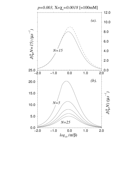
FIG. 3.: Flux as a function of effective pore-solvent binding $\bar{\alpha}$. We use representative values $dt\simeq 10$fs, $p=\beta_{0}=0.003$, and $\mbox{X}=\chi_{s}^{R}\simeq 0.0018$, corresponding to osmosis from pure solvent to a 100mM solute solution. (a). $J(\xi,N=15)$ is shown for $\alpha_{0}=0.001$(solid curve) and $\alpha_{0}=0.0045$(dashed curve) which give difference maxima at $\bar{\alpha}^{*}(\alpha_{0})$ and $\bar{\alpha}^{*}(\beta_{0})$ respectively. (b) shows $J$ for $N=5,10,15,20,25$ when $\alpha_{0}=0.001$. Note the discontinuities in slope at $\log(1/3)$ corresponding to the point where the source of increasing affinity switches from the increasing of $\alpha$ to the decreasing of $\beta$. (Figure 2(b).)

Figure 3 shows the current as the solvent-pore affinity is increased according to $\bar{\alpha}$, as $\bar{\alpha}=\alpha_{0}/\beta\rightarrow\alpha_{0}/\beta_{0}(\equiv\bar{\alpha}_{0})\rightarrow\alpha/\beta_{0}$. The solute concentration is represented in molar units $\left[c_{s}\right]=\chi_{s}^{R}\times 55.56$, such that a 100mM aqueous solute solution corresponds to $\mbox{X}=\chi_{s}^{R}\simeq 0.0018$. Although $J$ and $\xi$ can all be rescaled by the constant $p$, for concreteness and comparison with experiments, we consider a time step $dt\simeq 10\mbox{fs}\ll\tau_{p}\approx 0.3$ps, which sets $\beta_{0}\approx p\simeq 0.003$ and yields flows in the range of $10^{8}\times J$ (particles per $\mu$s) in good agreement with $P_{os}\sim 10^{-14}$cm³/s measured across aquaporin water channels with physiological ($\sim 100$mM) osmolyte solutions [2, 4].

Figure 3(a) plots the flux ($\mu\mbox{s}^{-1}$) as a function of $\log\bar{\alpha}$ for two different values, $\alpha_{0}/\beta_{0}=0.001/0.003<(\alpha/\beta_{0})^{*}=\sqrt{8/7(1-\mbox{X})}$ and $\alpha_{0}/\beta_{0}=0.0045/0.003>(\alpha/\beta_{0})^{*}$. At $\log(1/3)$, the curve bifurcates into the two solutions corresponding to either decreasing $\alpha$ or increasing $\beta$, with maxima determined by (14) and (15) respectively. The discontinuity in slope at $\log(1/3)$ (dashed curve) is apparent, although the one at $\log(3/2)$ near the maximum is not. Figure 3(b) compares $J(\xi,N)$ for various pore lengths $L=N\ell$ at $\alpha_{0}=0.001$ (such that (15) pertains). Whether $\alpha_{0}/\beta_{0}$ is greater or less than $\bar{\alpha}^{*}(\beta_{0})$ depends on the reservoir number density and $A_{p}$; for gases, $\alpha_{0}\ll\beta_{0}$ and a curve with maximum defined by (15) obtains. However, dense liquids entering large pores may have relatively large entrance rates such that $\alpha_{0}/\beta_{0}\gtrsim\bar{\alpha}^{*}(\beta_{0})$ and $J(\xi,N)$ may have a maximum defined by (14). From (14), this latter condition is less likely for larger driving X, and thus $\bar{\alpha}^{*}(\beta_{0})$.

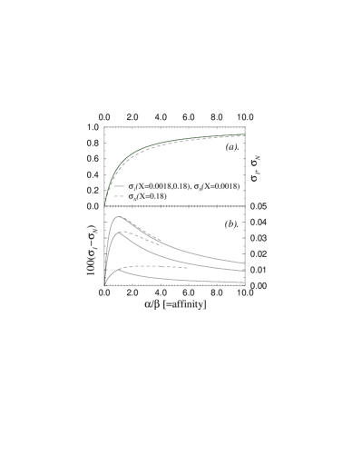
FIG. 4.: Occupations $\sigma$ for $p=\beta_{0}=\alpha_{0}=0.003$. (a) Pore occupations for $\mbox{X}=0.0018$ are all indistinguishable on this scale (solid curve). Only at $\mbox{X}=0.18$(10M solution) is $\sigma_{N=30}$ (dashed curve) sufficiently different from $\sigma_{1}$. (b) 100$\times(\sigma_{i}-\sigma_{N})$ as a function of $\alpha/\beta$ for $p=0.003,0.03,0.3$. Note the different behavior when $\alpha=\alpha_{0}=0.003$ at $\alpha/\beta=1.0$. The dashed fragments represent the occupation differences if $\alpha_{0}>0.003$.

Figure 4(a) shows the average occupation $\sigma_{i}(\bar{\alpha})$ for $\mbox{X}=\chi_{s}=0.0018$. The dependence on spatial position $i$ is weak and is not apparent on the scale of Fig. 4(a), except if $\mbox{X}=0.18$ (corresponding to 10M solutions) when $\sigma_{N}$ can be distinguished from $\sigma_{1}$. Therefore, from Eqn. (7) $\alpha/(\alpha+\beta)$ is an approximate value of averaged occupations at small X. The small difference in occupation along the chain is consistent with the assumption of local thermodynamic equilibrium. Figure 4 shows the difference $10^{3}\times(\sigma_{1}(\bar{\alpha})-\sigma_{N}(\bar{\alpha}))$ with $\alpha_{0}/\beta_{0}=1.0$ (solid curves). The dashed curves represent the occupation difference $10^{3}\times(\sigma_{1}-\sigma_{N})$ if $\alpha_{0}/\beta_{0}\gg 1$.

The behavior of $J(\xi,N)$ as a function of affinity $\bar{\alpha}$ can be further understood in terms of the associated pore occupations. At low $\bar{\alpha}$, the pore is repelling and contains few if any particles that can be transported. At high affinities, and occupations, most internal hopping steps are not fulfilled due to occupied neighboring sites choking off the flow. Only at intermediate $\bar{\alpha}$ and near (14) or (15), and intermediate occupations will maximum flow occur. At larger X, $\sigma_{N}$ decreases (see Fig. 4(a)), decreasing overall pore occupation and increasing the critical affinities $\bar{\alpha}^{*}(\beta_{0})$ and $\bar{\alpha}^{*}(\alpha_{0})$ where the maximum occurs. Therefore, the condition represented by (15) becomes more relevant for larger osmotic pressures.

FIG. 5.: The driving force dependence of $J(\xi,20)$ for osmosis from pure solvent to solution with $p=\beta_{0}=0.003$ and $\alpha_{0}=0.002$. Various values of $\bar{\alpha}=\alpha/\beta$ are shown. (a) For solute concentrations $\lesssim 5$M, the current is linear in $\mbox{X}=\chi_{s}^{R}$. (b) At higher solute concentrations, nonlinearities in $J(\xi,20)$ arise, particularly for high values of $\bar{\alpha}$ an pore occupation.

Figures 5 show the particle flux per microsecond, $10^{8}\times J(\xi,N=20)$, as a function of $\mbox{X}\simeq\chi_{s}^{R}$ at $\beta_{0}=p=0.003,\,\alpha_{0}=0.002$ for various pore-solvent affinities $\bar{\alpha}$. For the low values $\bar{\alpha}=0.01$(dashed curve) and $\bar{\alpha}=0.1$(dotted curve) the pore is repelling, while for $\bar{\alpha}=1.0$(solid curve) and $\bar{\alpha}=100$(thick curve) $\alpha=\alpha_{0}$ while $\beta$ decreases from $\beta_{0}$. The solid curve with $\bar{\alpha}=1.0$ is near the maximum defined by (15) while $\bar{\alpha}=100$ is within the choked flow limit represented by the decreasing branch on the high $\bar{\alpha}$ side of Figures 3(a,b). The flow is linear for low X as shown in 5(a). Figure 5(b) clearly shows that nonlinearities are important for large $\bar{\alpha}$ and that the flow for $\bar{\alpha}=1.0$(solid curve) is lower that that for $\bar{\alpha}=0.01$(dashed curve) only for small driving X. As the nonlinearity sets in for $\bar{\alpha}=1.0$, the flux increases faster than that for $\bar{\alpha}=0.01$ and surpasses it near X$\sim 3$. The flow nonlinearities shown in Fig 5(b) arise at large solute concentration differences and are only those resulting from the nonlinear dynamics determined by equations (3) and do not include solute nonidealities, unstirred layers, etc. That is, the coefficients

$$d_{k}={\bar{\alpha}^{k}p\left[(\bar{\alpha}+1)(N-1)+\bar{p}\right]^{k-1}\over(\bar{\alpha}+1)^{k}\left[(\bar{\alpha}+1)(N-1)+2\bar{p}\right]^{k}}$$ (16)

contain only the kinetic parameters describing the solvent-pore interactions. Furthermore, our treatment for $\alpha$ and $\beta$ assume thermodynamic equilibrium, or no unstirred/polarization layers. The modifications necessary to include unstirred layers are treated in the following paper.

From the denominator of (13), $J$ is linear in X for $\bar{\alpha}\mbox{X}/(\bar{\alpha}+1)\ll 1$. From (7), we see that $\bar{\alpha}/(\bar{\alpha}+1)$ is the average occupation for small $J$. Therefore, nonlinearities are important only when occupation $\sigma_{i}$ is high, when exclusion interactions, and thus nonidealities, are most pronounced (the $\bar{\alpha}=1.0,100$ curves in Fig. 5(b)). Although Eqn. (13), or (16) fully describes particle exclusion nonidealities within the pore, for the small $\Delta\chi_{s}$ usually encountered, a linear relationship,

$$J(\xi,N)\simeq{\bar{\alpha}\over\bar{\alpha}+1}{p\Delta\chi_{s}\over(N-1)(\bar{\alpha}+1)+2\bar{p}}$$ (17)

is accurate as demonstrated by Fig 5(a). In the limit $\bar{p}\ll(\bar{\alpha}+1)N$, $P_{os}$ approaches

$$P_{os}\cong\left({a\over L}\right){\alpha\bar{p}\over(\bar{\alpha}+1)^{2}n_{T}}.$$ (18)

In this limit(18), the “rate limiting steps” are the internal steps $(p)$ of pore particles, and the overall flux scales as $L^{-1}$. In the limit represented by (18), an Arrhenius temperature dependence of $(E_{\alpha}-E_{\beta}-E_{q})/k_{B}T\left[(E_{\beta}-E_{\alpha}-E_{q})/k_{B}T\right]$ is expected for $\bar{\alpha}\gg 1\left[\bar{\alpha}\ll 1\right]$.

According to the form of $\alpha_{0}$, $P_{os}\propto\alpha\bar{p}\propto r_{p}^{2}$ for $\bar{\alpha}\ll 1$, and $P_{os}\propto p/\bar{\alpha}\propto r_{p}^{-2}$ for $\bar{\alpha}\gg 1$. Note the curious $P_{os}\propto r_{p}^{-2}$ dependence indicating the $\bar{\alpha}>\bar{\alpha}^{*}$ regime shown by the large $\log_{10}\bar{\alpha}$ regions of Fig. 3 where decreasing $r_{p}$ (and $\alpha$) increases $\bar{J}$ by decreasing the high pore occupation.

Now consider the limit $\bar{p}\gg(\bar{\alpha}+1)N$. The rate limiting steps now involve pore entrance or exit and

$$P_{os}\cong{\alpha\over 2(\bar{\alpha}+1)n_{T}},$$ (19)

independent of $L$. This limit is equivalent to the single site $(N=1)$ model since only the boundary entrance and exit rates are relevant. The radius and temperature dependences in this case are $P_{os}\propto\alpha\propto r_{p}^{2}\exp(-E_{\alpha}/k_{B}T)$ and $P_{os}\propto\beta\propto\exp(-E_{\beta}/k_{B}T)$ for $\bar{\alpha}\ll 1$ and $\bar{\alpha}\gg 1$ respectively. Thus, the pore length $L\simeq N\ell$ can determine the temperature dependence of $J$ since it determines which of the two limits (18) or (19) is relevant. Except for experiments where lipids undergo phase transitions which affect the pore structure [33], a single exponential temperature dependence is almost always experimentally observed in biological systems involving osmosis [32], indicating one of the above limits for $P_{os}$ holds in the regimes explored. One interpretation is that a number of hydrogen bonds ($\sim 5k_{B}T$ each) must be broken before water can enter the pore. This is consistent with the identification of $E_{\alpha}$ as the energy required to break water H-bonds in the $\bar{\alpha}\ll 1$ limit of (18). Fluxes of nonpolar solvents through artificial pores may be expected to display richer temperature dependences since a wider variety of temperatures and molecular interactions can be accessed and experimentally probed.

B Pressure Driven Flow

For incompressible reservoirs without solutes, $\Delta\chi_{s}=\chi_{s}^{L}=\chi_{s}^{R}=0$; however, flow can be driven by differences in hydrostatic pressure. Hydrostatic pressure variations, rather than controlling the rates via the number density in the pre-exponential factors $\alpha_{0},\,\delta_{0}$, modify the relative activation energies $E_{\xi}$. For example, consider increasing $P^{L}$ keeping $P^{R}$ constant. For nearly incompressible liquids, the particle density changes negligibly, but their particle enthalpies increase as they are pushed against their interaction potentials. Changing the relative reservoir and pore enthalpies changes the entrance and exit kinetic coefficients according to Fig. 6(a), (b) for initially repelling or attractive pores.

FIG. 6.: Hydrostatic pressure increases in left reservoir. (a) In attractive pore, $\alpha=\delta$, $E_{\beta}$ is constant, and $E_{\gamma}=E_{\gamma}(P^{L})$. (b) For repelling pore, and small pressure differences (lower solid and dotted levels) $\gamma=\beta,\,E_{\delta}$ is fixed, and $E_{\alpha}=E_{\alpha}(P^{L})$. Pressure differences larger than $E_{\delta}$ result in $E_{\alpha}\approx 0$ and $E_{\gamma}=E_{\gamma}(P^{L})>0$.

Since we assume only $P^{L}$ is varied, $E_{\delta},\,E_{\beta}$ are kept constant, while $E_{\alpha}=E_{\alpha}(P^{L})$ and $E_{\gamma}=E_{\gamma}(P^{L})$. First consider an attractive pore where only $E_{\gamma}(P^{L})$ and $\gamma$ changes as $P^{L}$ is increased, as schematically depicted in Fig. 6(a). The flux is

$$\begin{array}[]{l}\displaystyle J\left(\gamma(P^{L}),N\right)=\\ \displaystyle\quad\quad{p\bar{\alpha}\mbox{X}\over(N-1)(\bar{\alpha}+1-\mbox{X})(\bar{\alpha}+1)+\bar{p}(2\bar{\alpha}+2-\mbox{X})}\end{array}$$ (20)

where

$$\mbox{X}(P^{L})\equiv 1-\exp\left[\Delta E/k_{B}T\right]$$ (21)

and $\Delta E\equiv E_{\beta}-E_{\gamma}(P^{L})$.

When hydraulic pressure pushes particles through a repelling pore, the current can be written in the form

$$\begin{array}[]{l}\displaystyle J\left(\alpha(P^{L}),\gamma(P^{L}),N\right)=\\ \displaystyle{p\bar{\delta}\mbox{X}\over(N-1)(\bar{\delta}+1)(\bar{\delta}+1-\mbox{X})+\bar{p}\left(\bar{\gamma}+\bar{\delta}+(\bar{\delta}+1)(1-\mbox{X})/\bar{\gamma}\right)}\end{array}$$ (22)

where in this case,

$$\mbox{X}=1-\exp\left[(E_{\alpha}(P^{L})+E_{\beta}-E_{\gamma}(P^{L})-E_{\delta})/k_{B}T\right],$$ (23)

and $\bar{d}$ measures the solvent-pore affinity since $\bar{\alpha}$ is varying with pressure. For low pressure differences such that

$$P^{L}-P^{R}\ll E_{\delta}\left[\left({\partial\Delta E\over\partial\Delta P}\right)_{T,\Delta P=0}\right]^{-1}$$ (24)

flow across repelling pores can be further simplified since $\gamma=\beta$ as evident in the lower three pressures $P^{L}$ in Fig. 6(b). When the pressure pushes the enthalpy of the left bath above that of the pore, the full pressure dependence (22) is required. Equations (20) and (22), along with the equation of state of the solvent in the reservoirs completely determine the nonlinear flux-pressure relationship. However, for low pressures, a Taylor expansion about $P^{L}=P^{R}$ yields

$$\mbox{X}\approx-{\Delta P\over k_{B}T}\left({\partial\Delta E\over\partial\Delta P}\right)_{T,\Delta P=0}=-\tilde{v}{\Delta P\over k_{B}T},$$ (25)

where the last equality is valid for incompressible liquids and $\tilde{v}$ is the molecular volume of a solvent particle in the reservoirs (for H₂O, $\tilde{v}\simeq 3\times 10^{-23}\mbox{cm}^{3}$). Linearizing (20) and (22) about small pressure differences, and recalling that $\alpha\simeq\delta$, we find

$$L_{p}\cong{P_{os}\over k_{B}T}$$ (26)

as required by linear nonequilibrium thermodynamics. However, differences between hydraulically driven and osmotically driven transport arise at higher order in X, as explicitly calculated in (6), (20), and (22).

Continuum Poiseuille flow (zero Reynolds number solution of the Navier-Stokes equation for flow through an infinite right circular cylinder[19]) expressions (where $J\propto r_{p}^{4}$) have been proposed to describe transport through microscopic channels. Although these continuum relations have no validity in microscopic settings, they are nevertheless often used to obtain estimates of permeabilities, pore radii [20], and membrane pore densities. These estimates typically do not agree well with independent measurements of pore radii and pore permeabilities[20]. Although the $r_{p}$ dependences in our model are valid only for a limited range of pore radii, they are consistent with the inapplicability, at microscopic scales, of the continuum expression $P_{os}\propto r_{p}^{4}/(\eta L)$, where $\eta$ is the bulk solvent viscosity.

Fluid flow through small orifices has been described as being both “viscous” and “diffusive.” Even though the limit (18) appears to be “viscous” due to the $L^{-1}$ dependence, and and (19) “diffusive,” we see that both pressure and osmosis driven flows in the present model is diffusive in nature. Consider the time averaged rate equation for occupation at site $i$,

$$\begin{array}[]{ll}\displaystyle\dot{\sigma}_{i}&\displaystyle=-p\sigma_{i}(1-\sigma_{i+1})-p\sigma_{i}(1-\sigma_{i-1})\\ &\hskip 50.58878pt+p(1-\sigma_{i})(\sigma_{i+1}+\sigma_{i-1})\\[13.0pt] &\displaystyle=p(\sigma_{i+1}-2\sigma_{i}+\sigma_{i-1})\end{array}$$ (27)

which on scales $\gg\ell$ is a diffusion equation with $p\ell^{2}\cong D_{c}$ a cooperative diffusion coefficient. When particles interact along the chain the overall flux is determined by the cooperative diffusion of particles. In the simple one-dimensional model presented, cooperative diffusion is related directly to the precisely defined dynamical rules (3), but in general is defined by linear density-density correlation functions, or Green-Kubo relations.

The neglect of true convective, or momentum transfer effects can be neglected in the systems we consider. The signature of convective flow, such as Poiseuille flow, is a particle velocity distribution function with is Maxwellian centered about a small finite stream velocity. However, in 1D, or nearly 1D pores, the particles thermally equilibrate with the stationary pore walls very quickly and are unable to collectively transfer a stream momentum. This is particularly valid for repelling pores where entropic pressure results in low pore occupations $\sigma_{i}\ll 1$. In this large Knudsen number regime [6], the particles will collide with walls more often that with neighboring particles.

IV Extensions and Conclusions

An extension of the 1D chain represented by (3) to include a distribution of site-dependent internal hopping rates $p_{i}=q_{i}$ can be straightforwardly calculated, as outlined in the Appendix. Biological realizations of internal pore defects with site dependent hopping rates are gramicidin A channels comprising of two barrel structures joined at the defect (membrane bilayer midplane)[1]. Similarly, water permeation through a bilayer membrane can be viewed as pores along the hydrophobic lipid tails with the bilayer midplane and possible unsaturated bonds acting like defects. Channel proteins with widely varying internal interactions would also be modified according to the results found in the Appendix. Strong particle-pore interactions which are incommensurate with $\ell$ may also lead to nonlinear transport. Here, possible cluster diffusion [31] and locked-sliding phases such as that found in Frenkel-Kontorowa [34] and friction models [35] can also affect transport. These effects offer the possibility of interesting nonlinearities amenable to numerical study. Solvents that have strong mutual attractive interactions can also be considered. For example, a particle may hop with different rates into an empty site at $i+1$ depending on whether or not there is an attractive particle behind it, at site $i-1$. The probability of such a hop to the right from $i\rightarrow i+1$ can be represented by $p\sigma_{i}(1-\sigma_{i+1})(1-\sigma_{i-1})+p^{\prime}\sigma_{i}(1-\sigma_{i+1})\sigma_{i-1}$ where $p$ represents the rate of an isolated particle, while $p^{\prime}\ll p$ represents the rate in the presence of another particle at $i-1$ binding to and preventing the hop of the particle at $i$ to $i+1$. The resulting particle density profile along the chain will no longer be linear. These effects offer the possibility of interesting nonlinearities amenable to numerical study.

For pores that are slightly larger, with radii larger than a few times the particle diameters, similar stochastic treatments can be applied provided particle momenta relax much faster than particle positional degrees of freedom. Only then is the collective stream velocity zero, and $p=q$ can be invoked. Near the single file limit, the pore walls are in constant interaction with the transported molecules and randomizing their momentum. Nevertheless, for larger pores, we can estimate the relative rates of positional and momentum relaxation. Pressure (either hydrostatic or osmotic) driven flow through a macroscopic circular pipe is described by Poiseuille’s law [19]

$$v(r)={\Delta P\over 4\eta L}(r_{p}^{2}-r^{2})$$ (28)

where $v(r)$ is the fluid element velocity along the pipe, and $\eta$ is the bulk fluid viscosity. Equation (28) has often been extended to describe flow through microscopic pipes, especially biological membrane pores, having radii $r_{p}$ of Angstroms. This is the origin of the notion that osmosis through microscopic pores is “convective.” However, for the Poiseuille stream convection to be comparable to “driven diffusive transport,” the ratio

$$\mbox{Pe}\equiv{vL\over D_{c}}\simeq{\Delta Pr_{p}^{2}\over 4\eta D_{c}}\sim 1,$$ (29)

where $D_{c}$ is the effective collective diffusion coefficient which describes dissipative particle density relaxation, and is also approximately the momentum diffusion, or sound attenuation coefficient. For a hydrostatic pressure difference of $\Delta P=2.5$ atm (corresponding to a 100mM solute concentration difference), and bulk viscosity and attenuation coefficient $\eta=0.01$g cm/s, and $D_{c}\simeq\eta/\rho$, convective, or “viscous”[14] flow will be irrelevant for $r_{p}\ll 1000\mbox{\AA}$. For typical zeolites and biological pores under the above conditions, $r_{p}\sim 3-8\mbox{\AA}$, $\mbox{Pe}\sim 10^{-5}\ll 1$. Thus, “convective” flow described by (28) is negligible compared to diffusive transport in systems of present concern. Diffusive transport in this context should not be confused with tracer diffusion or collective diffusion in binary mixtures, rather, it is the consequence of microscopic momentum relaxation due to frequent collisions with the pore interior. These collisions increase relative to particle-particle interactions for smaller and smaller pores, where the inner surface to pore volume ratio increases.

Additional support for the basic assumption of diffusive particle motions is found from nonequilibrium molecular dynamics studies (NEMD) of flow through a slit [14] where an external driving force $q\neq p$ was not used explicitly. However, the two reservoirs were held at different chemical potentials, or pressures. The density profile for Lennard-Jones particles with attraction energies close to $k_{B}T$, driven across 50Ålong slits of widths $2.5$ times the particle diameters with a 35 atm hydrostatic pressure difference was found to be linear, suggesting validity of (7) and Fick’s law even under extreme conditions [14]. The validity of (29) and diffusive ($p=q$) flow suggest that pores with radii $\sim 10-50\mbox{\AA}$ a few times molecular diameters can also be treated by multidimensional exclusion models consisting of a series of 1D chains with particle interchange among them. Solvent-solvent attractive interactions and diffusion of small clusters can also be straightforwardly implemented.

Although we have treated only a single pore, actual experiments measure flow over an area containing an ensemble of pores. The averaged steady state flux neglecting unstirred layers would then be

$$\langle J\rangle=\sum_{N,\{p_{i}\}}f(N,\{p_{i}\})J(N,\{p_{i}\})$$ (30)

where $f(N,\{p_{i}\})$ is the number distribution for pores of length $N$, with the set $\{p_{i}\}$ of internal defects. The pores in (30) need not be straight, and the sum over $N\simeq d/\ell\rightarrow\infty$ represents a distribution of pores with various total arc-lengths traversing a membrane of thickness $d$. We have not considered the nonlinear effects of solute-pore interactions, which we treat in detail in the companion paper.

The main results of this study is a thermodynamically consistent model of osmosis and pressure driven flows through nanoscopic-sized pores. All parameters in the theory are microscopically motivated yet are general enough to allow predictions in trends and identify correlations between transport rates and macroscopic thermodynamic properties. Predictions from this transport model are the site occupancies (7), the dependences of X on $\Delta\chi_{s}$ and $\Delta P=P^{R}-P^{L}$, the Arrhenius temperature dependences, the pore radius $r_{p}$ dependences, and the flow maximum (14-15) as a function of pore-solvent binding constant $\bar{\alpha}$. Also, microscopic expressions are derived for phenomenologically measured permeabilities $P_{os}$ and $L_{p}$. Equation (30), and the microscopically estimated values for the parameters involved offer an reasonable, semi-quantitative description of osmosis and pressure-driven flow through microscopic channels. The analytic model presented provides a simple, physically motivated analysis that complements more complicated numerical simulations by predicting rich parameter dependences.

A Flow through disordered pores

The exact steady state flow through a pore with random internal hopping rates $q_{i}=p_{i}$ can be found by extending the uniform pore solution (13). When these random hopping rates are time independent, or fluctuate independently of the particle occupations $\sigma$, the steady state between section $i$ and $i+1$ is

$$J_{i}=p_{i}(\sigma_{i}-\sigma_{i+1})$$ (A1)

and the mean-field solution becomes exact. Summing (A1) across the channel yields

$$J\sum_{i=1}^{N-1}p_{i}^{-1}=\sigma_{1}-\sigma_{N},$$ (A2)

which upon solving with (7) for $J$,

$$J={\alpha\beta-\gamma\delta\over(\alpha+\gamma)(\beta+\delta)\sum_{i=1}^{N-1}p_{i}^{-1}+(\alpha+\beta+\gamma+\delta)}.$$ (A3)

The above result also constitutes a steady state solution to the XXZ spin chain Hamiltonian [36] with site-dependent energies.

REFERENCES

- [1] B. Alberts, D. Bray, J. Lewis Molecular Biology of the Cell, (Garland, 1994)
- [2] A. Finkelstein, Water Movement Through Lipid Bilayers, Pore, and Plasma Membranes, (Wiley-Interscience, New York, 1987).
- [3] R. M. Barrer, Zeolites and Clay Minerals as Sorbents and Molecular Sieves, (Academic Press, London, 1978).
- [4] T. Zeuthen, “Molecular Mechanisms for Passive and Active Transport of Water,”Int. Rev. Cyt., 160, 99-160, (1995).
- [5] J. Kärger, M. Petzold, H. Pfeifer, S. Ernst, and J. Weitkamp, “Single-file Diffusion and Reaction in Zeolites,” J. Catalysis, 136, 283-299, (1992).
- [6] E. L. Cussler, Diffusion: Mass Transfer in Fluid Systems, (Cambridge University Press, Cambridge, 1984).
- [7] H. C. Longuet-Higgins and G. Austin, “The kinetics of osmotic transport through pores of molecular dimensions,”Biophys. J., 6, 217-224, (1966).
- [8] S. Nivarthi, A. V. McCormick, H. T. Davis, Chem. Phys. Lett., 229, 297, (1994); V. Gupta, S. S. Nivarthi, A. V. McCormick, H. T. Davis, Chem. Phys. Lett., 247, 596, (1995)
- [9] S. Murad, P. Ravi, and J. G. Powles, “A computer simulation study of fluids in model slit, tubular, and cubic micropores,” J. Chem. Phys., 98(12), 9771, (1993).
- [10] C. Rödenbeck, J. Kärger, and K. Hahn, “Exact analytical description of tracer exchange and particle conversion in single-file systems,” Phys. Rev. E, 55(5), 5697-5712, (1997).
- [11] S. G. Kalko, J. A. Hernandez, J. R. Grigera and J. Fischbarg, “Osmotic permeability in a molecular dynamics simulation of water transport through a single-occupancy pore,” Biochim. et Biophys. Acta-Biomembranes, 1240(2), 159-166, (1995).
- [12] J. A. Hernandez and J. Fischbarg, “Kinetic analysis of water transport through a single file pore,” J. Gen. Physiol., 99(4), 645-662, (1992).
- [13] H.-H. Kohler and K. Heckmann, “Unidirectional fluxes in staurated single-file pores of biological and artificial membranes. I. Pores containing no more than one vacancy,” J. Theor. Biol., 79, 381-401, (1979).
- [14] R. F. Cracknell, D. Nicholson, and N. Quirke, “Direct Molecular Dynamics Simulation of Flow Down a Chemical Potential Gradient in a Slit-Shaped Pore,” Phys. Rev. Lett., 74(13), 2463-2466, (1995).
- [15] S. Bandyopadhyay, and S. Yashonath, “Diffusion Anomaly in Silicalite and VPI-5 from Molecular Dynamics Simulations,” J. Phys. Chem., 99, 4286-4292, (1995).
- [16] T. Chou, “How fast do fluids squeeze through microscopic single-file pores,” Phys. Rev. Lett. 80(1), 85-88, (1998).
- [17] D. C. Guell and H. Brenner, “Physical Mechanism of Membrane Osmotic Phenomena,” Ind. Eng. Chem. Res., 35, 3004-3014, (1996).
- [18] L. E. Reichl, A modern Course in Statistical Physics, (University of Texas Press, Austin, 1980).
- [19] L. D. Landau and E. M. Lifshitz, Fluid Mechanics (Pergamon Press, New York, 1985).
- [20] W. R. Galey and J. Brahm, “The failure of hydrodynamic analysis to define pore size in cell membranes,” Biochim. et Biophysica Acta, 818, 425-428, (1985).
- [21] Z. Y. Yan, S. Weinbaum, and R. Pfeffer, “On the fine structure of osmosis including 3-dimensional pore entrance and exit behavior,” J. Fluid Mech., 162, 415-438, (1986)
- [22] H. Wang and R. Skalak, “Viscous flow in a cylindrical tube containing a line of sherical particles,” J. Fluid Mech., 38, 75-96, (1969).
- [23] S. Sokolowski, “Molecular dynamics studies of adsorption and flow of fluids through geometrically non-uniform cylindrical pores,” Molecular Physics, 75(6), 1301-1327, (1992).
- [24] L. D. Gelb, and K. E. Gubbins, “Liquid-liquid phase separation in cylindrical pores: Quench molecular dynamics and Monte Carlo simulations,” Phys. Rev. E, 56(3), 3185-3196, (1997).
- [25] J. Koplik, J. R. Banavar, and J. F. Willemsen, Phys. Fluids A, 1(5), 781, (1989); S. Sokolowski, Molecular Phys., 75(6), 1301, (1992).
- [26] A. Cheng, A. N. van Hoek, M. Yeager, A. S. Verkman, and A. K. Mitra, “Three-dimensional organization of a human water channel,” Nature, 387, 627-630, (1997).
- [27] B. K. Jap and H. Li, “Structure of the osmo-regulated H2O-channel AQP-CHIP in projection at 3.5 resolution,” J. Mol. Biol., 251, 413-420, (1995).
- [28] R. B. Stinchcombe and G. M. Schültz, Phys. Rev. Lett., 75, 140, (1995); Nonequilibrium Statistical Mechanics in One Dimension, Ed. V. Privman, (Cambridge University Press, 1997).
- [29] B. Derrida, S. A. Janowsky, J. L. Leibowitz, and E. R. Speer, “Exact Solution of the Totally Asymmetric Simple Exclusion Process: Shock Profiles,” J. Stat. Phys.,73, 813-842, (1993).
- [30] M. P. Allen and D. J. Tildesley, Computer Simulation of Liquids, (Oxford University Press, Oxford, 1987).
- [31] D. S. Sholl and K. A. Fichthorn, “Concerted Diffusion of Molecular Clusters in a Molecular Sieve,” Phys. Rev. Lett., 97(19), 3569-3572, (1997).
- [32] B. E. Cohen, “The permeability of liposomes to nonelectrolytes: 1. Activation energies for permeation,” J. Membr. Biol., 20, 205-234, (1975); “The permeability of liposomes to nonelectrolytes: 2. The effect of nystatin and gramicidin A,” 20, 235-268, (1975).
- [33] B. A. Boehler, J. de Gier, L. L. M. van Deenen, “The Effect of Gramicidin A on the Temperature Dependence of Water Permeation Through Liposomal Membranes Prepared from Phosphatidylcholines with Different Chain Lengths,” Biochimica et Biophysica Acta, 512, 480-488, (1978).
- [34] Chaikin, P. M. and Lubensky, T. 1995 Principles of condensed matter physics, (Cambridge University Press, Cambridge, 1995)
- [35] Z. Csahok, F. Family, T. Vicsek, “Transport of Elastically Coupled Particles in an Asymmetric Periodic Potential, Phys. Rev. E, 55(3), 3598-3612, (1997); O. M. Braun, T. Dauxois, M. V. Paliy, and M. Peyrard, “Nonlinear mobility of the generalized Frenkel-Kontorova model,” ibid. pp. 3598-3612.
- [36] S. Sandow, “Partially asymmetric exclusion process with open boundaries,” Phys. Rev. E, 50(4), 2660-2667, (1994).