Statics and dynamics of an Ashkin-Teller neural network with low loading

An Ashkin-Teller neural network, allowing for two types of neurons is considered in the case of low loading as a function of the strength of the respective couplings between these neurons. The storage and retrieval of embedded patterns built from the two types of neurons, with different degrees of (in)dependence is studied. In particular, thermodynamic properties including the existence and stability of Mattis states are discussed. Furthermore, the dynamic behaviour is examined by deriving flow equations for the macroscopic overlap. It is found that for linked patterns the model shows better retrieval properties than a corresponding Hopfield model.

PACS numbers: 87.10.+e, 02.50.+s, 64.60.Cn

1 Introduction

One of the best known physical models for neural networks is the Hopfield model [1]. In theoretical investigations of network properties, e.g., the retrieval of learned patterns, it plays a similar role as the Ising model does in the theory of magnetism. Extensions of this model to multi-state neurons have received a lot of attention recently (see, e.g., [2] - [5] and the references cited therein). Thereby the ability to store and retrieve so-called grey-toned and coloured patterns has been investigated.

In this work we consider another extension of the Hopfield model to allow for multi-functional neurons. The specific model we have in mind is the neural network version of the Ashkin-Teller spin-glass ([6]-[9]). Indeed, on the one hand the Ashkin-Teller model has two different kinds of neurons (spins) at each site interacting with each other. This allows us to interprete this model as a neural network with two types of neurons having different functions. On the other hand, this Ashkin-Teller neural network (ATNN) can be considered as a model consisting out of two interacting Hopfield models.

We expect the behaviour of the ATNN to be different from the one of the Hopfield model in a non trivial way. One of the things we want to find out, e.g., is whether this (four-neuron) interaction between the two types of neurons can improve the retrieval process for embedded patterns built from these two types of neurons. We will see, indeed, that for a particular choice of this interaction term the retrieval quality of the embedded patterns is very high in comparison with a corresponding Hopfield model. Therefore, independent of the possible biological relevance of this model, if any, such a study is interesting from the pure physical point of view.

In this work we consider both the thermodynamic and dynamic properties of this model in the case of loading of a finite number of patterns.

The rest of this paper is organized as follows. In section 2 the ATNN model is introduced. Section 3 discusses the methods used for analyzing both the equilibrium properties and the dynamics of the model. In particular, fixed-point equations as well as flow equations for the relevant macroscopic overlap order parameters are derived. In section 4 numerical solutions of these equations are discussed for a representative set of network parameters. The retrieval properties of embedded patterns with different degrees of dependencies are compared. Section 5 presents the main conclusions.

2 The model

We consider a network of $N$ sites. At each site we have two different types of binary neurons, $s_{i}$ and $\sigma_{i}\,\,,i=1,\ldots,N$. The two types of neurons interact via a four-neuron term $s_{i}s_{j}\sigma_{i}\sigma_{j}$. The infinite-range hamiltonian reads

$$H=-\frac{1}{2}\sum_{i,j}[J_{ij}^{(1)}s_{i}s_{j}+J_{ij}^{(2)}\sigma_{i}\sigma_{j}+J_{ij}^{(3)}s_{i}s_{j}\sigma_{i}\sigma_{j}]$$ (1)

In this network we want to store a finite number of patterns, $p$, also of two different types, i.e., $\mbox{\boldmath$\xi$}_{i}=\{\xi_{i}^{\mu}\},\mu=1,\ldots,p$ and $\mbox{\boldmath$\eta$}_{i}=\{\eta_{i}^{\nu}\},\nu=1,\ldots,p$, which are supposed to be independent identically distributed random variables (i.i.d.r.v.) taking the values $+1$ or $-1$ with probability $1/2$. To build in the capacity for learning and retrieval in this network its stable configurations must be correlated with the configurations determined by the learning process. This can be accomplished by taking the Hebb learning rule for the interactions

$$J_{ij}^{(1)}=\frac{1}{N}J_{1}\sum_{\mu=1}^{p}\xi_{i}^{\mu}\xi_{j}^{\mu},\quad J_{ij}^{(2)}=\frac{1}{N}J_{1}\sum_{\mu=1}^{p}\eta_{i}^{\mu}\eta_{j}^{\mu},\quad J_{ij}^{(3)}=\frac{1}{N}J_{3}\sum_{\mu=1}^{p}\gamma_{i}^{\mu}\gamma_{j}^{\mu}\,,$$ (2)

where the $\mbox{\boldmath$\gamma$}_{i}=\{\gamma_{i}^{\mu}\},\mu=1,\ldots,p$ are also i.i.d.r.v. taking the values $+1$ or $-1$ with probability $1/2$.

At this point some remarks are in order. Firstly, we have taken the strength of the two types of patterns to be equal, meaning that the ATNN model is isotropic. Secondly, it is clear that the behaviour of this model (1)-(2) might depend on the fact whether the $\gamma$ are taken to be independent from the $\xi$ and the $\eta$ or not. The following cases will be distinguished:

1. unlinked patterns

   1. $\mbox{\boldmath$\xi$}_{i},\mbox{\boldmath$\eta$}_{i}$ and $\mbox{\boldmath$\gamma$}_{i}$ are i.i.d.r.v.

   2. $\mbox{\boldmath$\xi$}_{i}=\mbox{\boldmath$\eta$}_{i}$ and $\mbox{\boldmath$\gamma$}_{i}$ are i.i.d.r.v.

   3. $\mbox{\boldmath$\xi$}_{i}=\mbox{\boldmath$\eta$}_{i}=\mbox{\boldmath$\gamma$}_{i}$ is i.i.d.r.v.

2. linked patterns
   $\gamma^{\mu}_{i}=\xi^{\mu}_{i}\eta^{\mu}_{i}$ with $\mbox{\boldmath$\xi$}_{i}$ and $\mbox{\boldmath$\eta$}_{i}$ i.i.d.r.v.

We note that this ATNN model can also be considered as an assembly of two single Hopfield models (when $J_{3}=0$), one in the $s_{i}$-neurons and one in the $\sigma_{i}$-neurons interconnected via a four-neuron interaction (when $J_{3}\neq 0$). The study of coupled Hopfield networks has aroused some interest in the literature before (e.g., [10]).

In the following we discuss both the thermodynamics and the dynamics of this ATNN neural network with low loading.

3 The method

3.1 Statics

Starting from the hamiltonian (1)-(2) and applying standard techniques (linearization and the saddle-point method [11]-[12]) the ensemble-averaged free energy is given by

$$f=\frac{1}{2}(J_{1}{\bf m}_{1}^{2}+J_{1}{\bf m}_{2}^{2}+J_{3}{\bf m}_{3}^{2})$$

$$-\frac{1}{\beta}\left\langle\!\left\langle\ln[4\cosh\beta L_{1}\cosh\beta L_{2}\cosh\beta L_{3}(1+\tanh\beta L_{1}\tanh\beta L_{2}\tanh\beta L_{3})]\right\rangle\!\right\rangle$$

(3)

with

$$L_{1}=J_{1}\mbox{\boldmath$\xi$}\cdot{\bf m}_{1},\quad L_{2}=J_{1}\mbox{\boldmath$\eta$}\cdot{\bf m}_{2},\quad L_{3}=J_{3}\mbox{\boldmath$\gamma$}\cdot{\bf m}_{3}\,.$$ (4)

In the above the double brackets $\langle\!\langle\cdot\rangle\!\rangle$ denote the average over the distribution of the embedded patterns. The ${\bf m}_{\alpha}=\{m_{\alpha}^{\mu}\},\mu=1,\ldots,p;\alpha=1,2,3$ are, as usual, overlap order parameters defined by

$${\bf m}_{1}=\frac{1}{N}\sum_{i=1}^{N}\mbox{\boldmath$\xi$}_{i}s_{i},\quad{\bf m}_{2}=\frac{1}{N}\sum_{i=1}^{N}\mbox{\boldmath$\eta$}_{i}\sigma_{i},\quad{\bf m}_{3}=\frac{1}{N}\sum_{i=1}^{N}\mbox{\boldmath$\gamma$}_{i}s_{i}\sigma_{i}\,.$$ (5)

Here we remark that in the thermodynamic limit $N\rightarrow\infty$ and for finite loading $\alpha=0$ the diagonal terms in the couplings, $J_{ii}$, do not play any role in the Hamiltonian (1).

In fact our model can be considered as a special case of the general spin-glass model presented in ref. [8] such that the expressions (3)-(4) can also be read off from there.

The fixed-point equations for the order parameters read

$${\bf m}_{\alpha}=\left\langle\!\left\langle\frac{\mbox{\boldmath$\psi$}_{\alpha}(\tanh\beta L_{\alpha}+\tanh\beta L_{\nu}\tanh\beta L_{\rho})}{1+\tanh\beta L_{\alpha}\tanh\beta L_{\nu}\tanh\beta L_{\rho}}\right\rangle\!\right\rangle\,,$$ (6)

where $\alpha,\nu,\rho=1,2,3$ are taken to be different and where $\mbox{\boldmath$\psi$}_{\alpha}$ is the embedded pattern corresponding to ${\bf m}_{\alpha}$.

Since the study of this ATNN model is very involved we have restricted ourselves here to a detailed treatment of the Mattis states ([12]) which are especially important from a neural network point of view. In our case they are defined as those solutions of the fixed-point equations for which not more than one component of each order parameter is different from zero, e.g. ${\bf m}_{1}=m_{1}(1,0,...,0)$, ${\bf m}_{2}=m_{2}(1,0,...,0)$, ${\bf m}_{3}=m_{3}(1,0,...,0)$. These states are denoted by $m_{1}m_{2}m_{3}$ in the sequel. We will see that those states are the only ones which contribute to the thermodynamics of the system. Solutions with more than one component being non-zero, i.e., mixture states will be important for the dynamics if they are local minima of the free energy.

For zero temperature we note that the eqs. (6) can be simplified by replacing the $\tanh\beta L_{\alpha}$ by $\mbox{\rm sign}L_{\alpha}$. Then it is straightforward to show that for each order parameter

$$({\bf m}_{\alpha})^{2}\leq 1\,,\quad\alpha=1,2,3\,,$$ (7)

with the equality being satisfied for a one-component ${\bf m}_{\alpha}$, and that the ground-state energy is given by

$$E=-\sum_{\alpha=1}^{3}\frac{1}{2}{\bf m}_{\alpha}^{2}\,.$$ (8)

In section 4 we report on the existence and stability of these Mattis states as a function of the temperature.

3.2 Dynamics

The analysis outlined above enables us to find the local minima of the free energy. But in order to find out how an arbitrary initial state of the network changes in time and to what extent, if at all, one of the learned patterns is approached, we derive a flow equation for the overlap order parameters.

We consider sequential updating of the spins consistent with the detailed balance condition. Hence we choose the following transition probabilities for a spin flip at a certain time step

$$\omega_{1}(s_{i},\sigma_{i}) \equiv \omega(s_{i}\rightarrow-s_{i})=\frac{1}{12}[1-\tanh(\beta(s_{i}h^{(1)}_{i}+s_{i}\sigma_{i}h^{(3)}_{i}))]$$

$$\omega_{2}(s_{i},\sigma_{i}) \equiv \omega(\sigma_{i}\rightarrow-\sigma_{i})=\frac{1}{12}[1-\tanh(\beta(\sigma_{i}h^{(2)}_{i}+s_{i}\sigma_{i}h^{(3)}_{i}))]$$

$$\omega_{3}(s_{i},\sigma_{i}) \equiv \omega(s_{i}\rightarrow-s_{i},\sigma_{i}\rightarrow-\sigma_{i})=\frac{1}{12}[1-\tanh(\beta(s_{i}h^{(1)}_{i}+\sigma_{i}h^{(2)}_{i}))]$$ (9)

with the $h_{i}$ appropriate local fields acting on the neurons in the following way

$$h^{(1)}_{i}=\frac{J_{1}}{N}\sum_{j}\sum_{\mu}\xi_{i}^{\mu}\xi_{j}^{\mu}s_{j},\,\,h^{(2)}_{i}=\frac{J_{2}}{N}\sum_{j}\sum_{\mu}\eta_{i}^{\mu}\eta_{j}^{\mu}\sigma_{j},\,\,h^{(3)}_{i}=\frac{J_{3}}{N}\sum_{j}\sum_{\mu}\gamma_{i}^{\mu}\gamma_{j}^{\mu}s_{j}\sigma_{j}\,,$$ (10)

where, as in the treatment of the statics we take $J_{1}=J_{2}$. At this point we remark that in the thermodynamic limit $N\rightarrow\infty$ the diagonal terms in the couplings, $J_{ii}$, do not survive. Furthermore we note that the method used here is also valid in the case of unequal $J$.

We then consider the probability $p({\bf s},\mbox{\boldmath$\sigma$};t)$ that the system is in a state ${\bf s}=(s_{i},...,s_{N})$, $\mbox{\boldmath$\sigma$}=(\sigma_{1},...,\sigma_{N})$ at time $t$. It satisfies the master equation

$$\frac{\partial p({\bf s},\mbox{\boldmath$\sigma$};t)}{\partial t} = \sum_{i=1}^{N}\left\{\omega_{1}(F_{i}^{1}s_{i},\sigma_{i})p(F_{i}^{1}\{{\bf s},\mbox{\boldmath$\sigma$}\};t)+\omega_{2}(s_{i},F_{i}^{2}\sigma_{i})p(F_{i}^{2}\{{\bf s},\mbox{\boldmath$\sigma$}\};t)\right.$$ (11)

$$+ \left.\omega_{3}(F_{i}^{3}s_{i},F_{i}^{3}\sigma_{i})p(F_{i}^{3}\{{\bf s},\mbox{\boldmath$\sigma$}\};t)\right.$$

$$- \left.p({\bf s},\mbox{\boldmath$\sigma$};t)[\omega_{1}(s_{i},\sigma_{i})+\omega_{2}(s_{i},\sigma_{i})+\omega_{3}(s_{i},\sigma_{i})]\rule{0.0pt}{14.22636pt}\right\}\,.$$

The operator $F_{i}^{\nu}$, $\nu=1,2,3$ acting on a configuration $\{{\bf s},\mbox{\boldmath$\sigma$}\}$ changes the sign of the following spins: $s_{i}$ for $\nu=1$, $\sigma_{i}$ for $\nu=2$ and simultaneously $s_{i}$ and $\sigma_{i}$ for $\nu=3$.

¿From this we want to derive a flow equation for the overlap order parameters. Because of the multi-state character of the model (due to the four-spin interaction term) the summation over $i$ has to be carried out by generalizing the method of submagnetizations or suboverlaps connected with partitions of the network with respect to the built-in patterns [13]-[14]. We note that for Hopfield networks we do not need such a partitioning [15].

First we introduce the following division of the network indices

$$\{i\leq N\}=\bigcup_{{\bf k}}I_{{\bf k}}\quad I_{{\bf k}}=\{i\leq N;{\bf k}={\bf k}_{i}\}\quad{\bf k}_{i}=(\mbox{\boldmath$\xi$}_{i},\mbox{\boldmath$\eta$}_{i},\mbox{\boldmath$\gamma$}_{i})\,.$$ (12)

Then we define the so called submagnetisations or suboverlaps

$$\mu_{\alpha,{\bf k}}({\bf s},\mbox{\boldmath$\sigma$})=\frac{1}{|I_{{\bf k}}|}\sum_{i\in I_{{\bf k}}}S_{\alpha,i}\quad\alpha=1,2,3\quad S_{1,i}=s_{i},~{}S_{2,i}=\sigma_{i},~{}S_{3,i}=s_{i}\sigma_{i}~{},$$ (13)

which enables us to write the overlaps in the form

$$m_{\alpha}^{\nu}=\sum_{{\bf k}}\frac{|I_{{\bf k}}|}{N}\mu_{\alpha,{\bf k}}k^{(\alpha-1)p+\nu}\quad\alpha=1,2,3,\quad\nu=1,...,p\,,$$ (14)

where $|I_{k}|$ stands for the number of indices in the set $I_{k}$. The number of vectors ${\bf k}$ is equal to $2^{ap}$, which is much smaller than the number $N$ of sites $i$ (when $N\rightarrow\infty$). The coefficient $a=3,2,1$ and $2$ for patterns of type $1(a),1(b),1(c)$ and $2$ respectively. So, an embedded random pattern configuration can be assumed to be equally distributed over the sets $I_{k}$ such that $|I_{k}|=2^{-ap}N+{\cal O}(N^{1/2})$.

Next we write down the probability $P(\mbox{\boldmath$\mu$};t)$ that the system is in a macroscopic state described by a set of submagnetisations $\mbox{\boldmath$\mu$}({\bf s},\mbox{\boldmath$\sigma$})\equiv\{\mu_{\alpha,{\bf k}}\}$

$$P(\mbox{\boldmath$\mu$};t)=\sum_{\{{\bf s},\mbox{\boldmath$\sigma$}\}}p({\bf s},\mbox{\boldmath$\sigma$};t)\delta(\mbox{\boldmath$\mu$}-\mbox{\boldmath$\mu$}({\bf s},\mbox{\boldmath$\sigma$}))\,.$$ (15)

Then we arrive at the following master equation (cfr. eq. (11))

$$\frac{\partial P(\mbox{\boldmath$\mu$};t)}{\partial t}=\sum_{\{{\bf s},\mbox{\boldmath$\sigma$}\}}\sum_{i}\sum_{\nu}\omega_{\nu}(s_{i},\sigma_{i})p_{t}({\bf s},\mbox{\boldmath$\sigma$})\left[\delta(\mbox{\boldmath$\mu$}-\mbox{\boldmath$\mu$}(F_{i}^{\nu}\{{\bf s},\mbox{\boldmath$\sigma$}\}))-\delta(\mbox{\boldmath$\mu$}-\mbox{\boldmath$\mu$}({\bf s},\mbox{\boldmath$\sigma$}))\right]\,.$$ (16)

The action of the operator $F_{i}^{\nu}$ can be specified further by writing

$$\mbox{\boldmath$\mu$}(F_{i}^{\nu}\{{\bf s},\mbox{\boldmath$\sigma$}\})=\mbox{\boldmath$\mu$}({\bf s},\mbox{\boldmath$\sigma$})-{\bf R}^{\nu}(s_{i},\sigma_{i})\,.$$ (17)

It is then straightforward to check that certain elements of the matrix $[{\bf R}^{\nu}(s_{i},\sigma_{i})]_{\alpha,{\bf k}}$ are zero, viz.

$$R^{1}_{2,{\bf k}}=R^{2}_{1,{\bf k}}=R^{3}_{3,{\bf k}}=0\quad\forall{\bf k},i\leq N\,.$$ (18)

Furthermore, for $\nu$ and $\alpha$ different from these specific values in (18) we have

$$R^{\nu}_{\alpha,{\bf k}}=\frac{2}{|I_{{\bf k}}|}S_{\alpha,i}\quad\mbox{if}\,\,\,i\in I_{{\bf k}}$$ (19)

$$R^{\nu}_{\alpha,{\bf k}}=0\quad\mbox{if}\,\,\,i\not\in I_{{\bf k}}\,.$$ (20)

In the thermodynamic limit $N\rightarrow\infty$ the parameters $\mu$ become continuous variables. Following [13] we then write for an arbitrary smooth function $\phi(\mbox{\boldmath$\mu$})$

$$\frac{\partial\langle\phi(t)\rangle}{\partial t} \equiv\int d\mbox{\boldmath$\mu$}\,\phi(\mbox{\boldmath$\mu$})\frac{\partial P(\mbox{\boldmath$\mu$};t)}{\partial t}$$ (21)

$$=\sum_{\{{\bf s},\mbox{\boldmath$\sigma$}\}}\sum_{i}\sum_{\nu}\int d\mbox{\boldmath$\mu$}^{{}^{\prime}}p({\bf s},\mbox{\boldmath$\sigma$};t)\delta(\mbox{\boldmath$\mu$}^{{}^{\prime}}-\mbox{\boldmath$\mu$}({\bf s},\mbox{\boldmath$\sigma$}))\omega_{\nu}(s_{i},\sigma_{i})$$

$$\times\left[\phi(\mbox{\boldmath$\mu$}^{{}^{\prime}}-{\bf R}^{\nu}(s_{i},\sigma_{i}))-\phi(\mbox{\boldmath$\mu$}^{{}^{\prime}})\right]\,.$$

Making an expansion of $\phi$ around $\mbox{\boldmath$\mu$}^{{}^{\prime}}$ and doing a partial integration with respect to $\mbox{\boldmath$\mu$}^{{}^{\prime}}$ we arrive at

$$\frac{\partial\langle\phi(t)\rangle}{\partial t}=\int d\mbox{\boldmath$\mu$}^{{}^{\prime}}\,\phi(\mbox{\boldmath$\mu$}^{{}^{\prime}})\sum_{\alpha,{\bf k}}\frac{\partial}{\partial\mu^{{}^{\prime}}_{\alpha,{\bf k}}}\left(\sum_{\{{\bf s},\mbox{\boldmath$\sigma$}\}}\sum_{i}\sum_{\nu}p({\bf s},\mbox{\boldmath$\sigma$};t)\delta(\mbox{\boldmath$\mu$}^{{}^{\prime}}-\mbox{\boldmath$\mu$}({\bf s},\mbox{\boldmath$\sigma$}))\right.$$

$$\left.\times R_{\alpha,{\bf k}}^{\nu}(s_{i},\sigma_{i})\,\omega_{\nu}(s_{i},\sigma_{i})\rule{0.0pt}{17.07182pt}\right)+{\cal O}(N^{-1})\,.$$ (22)

We remark that up to now we have not used the specific form for the transition probabilities $\omega_{\nu}$. Other expressions for $\omega_{\nu}$, satisfying detailed balance could also be employed.

Using the partitioning of the network into subsets $I_{{\bf k}}$ we can replace the sum over $i$ by $\sum_{{\bf k}}\sum_{i\in I_{{\bf k}}}$. Employing the specific form (9) for $\omega_{\nu}$ and performing the sum over $\{{\bf s},\mbox{\boldmath$\sigma$}\}$ we arrive at (compare [13])

$$\frac{\partial\langle\phi\rangle_{t}}{\partial t}=\int d\mbox{\boldmath$\mu$}\,\phi(\mbox{\boldmath$\mu$})\sum_{\alpha,{\bf k}}\frac{\partial}{\partial\mu_{\alpha,{\bf k}}}P(\mbox{\boldmath$\mu$};t)\left[\frac{1}{3}\mu_{\alpha,{\bf k}}-f_{\alpha,{\bf k}}(\{\mu_{\beta,{\bf k}}\})\right]\,,$$ (23)

where $f_{\alpha,{\bf k}}(\{\mu_{\beta,{\bf k}}\})$ is a function of all the suboverlaps given by

$$f_{\alpha,{\bf k}}(\{\mu_{\beta,{\bf k}}\}) =\frac{1}{12}\{\tanh(\beta L_{\alpha}+\beta L_{\nu})+\tanh(\beta L_{\alpha}-\beta L_{\nu})+\tanh(\beta L_{\alpha}+\beta L_{\rho})$$ (24)

$$+\tanh(\beta L_{\alpha}-\beta L_{\rho})+\mu_{\nu,{\bf k}}[\tanh(\beta L_{\alpha}+\beta L_{\rho})-\tanh(\beta L_{\alpha}-\beta L_{\rho})]$$

$$+\mu_{\rho,{\bf k}}[\tanh(\beta L_{\alpha}+\beta L_{\nu})-\tanh(\beta L_{\alpha}-\beta L_{\nu})]\}$$

with the $L_{\alpha}$ ($\alpha,\nu,\rho=1,2,3$ and different from each other) given by eq. (4). Since this equation holds for every smooth function $\phi$ the equation for the probabilities $P(\mbox{\boldmath$\mu$};t)$ has the form

$$\frac{\partial P(\mbox{\boldmath$\mu$};t)}{\partial t}=\sum_{\alpha,{\bf k}}\frac{\partial}{\partial\mu_{\alpha,{\bf k}}}P(\mbox{\boldmath$\mu$};t)\left[\frac{1}{3}\mu_{\alpha,{\bf k}}-f_{\alpha,{\bf k}}(\{\mu_{\beta,{\bf k}}\})\right]$$ (25)

and the corresponding flow equations for the submagnetisations $\mu_{\alpha,{\bf k}}$ themselves read

$$\frac{\partial\mu_{\alpha,{\bf k}}}{\partial t}=-\frac{1}{3}\mu_{\alpha,{\bf k}}+f_{\alpha,{\bf k}}(\{\mu_{\beta,{\bf k}}\})\,.$$ (26)

Together with (14) these coupled equations are used to study the dynamic behaviour of the network. In the following section the results of this study are discussed.

4 Results

In this section we discuss the numerical results for the ATNN model obtained from the fixed-point equations specifying the thermodynamic properties and from the flow equations for the suboverlaps describing the dynamics. We treat the cases of linked patterns and unlinked patterns separately. We report the results for a set of representative examples illustrating the main new features of the model.

4.1 Unlinked patterns

We first consider the model with equal coupling parameters $J_{3}=J_{1}(=J_{2})=1$. Introducing Mattis-type states $m_{1}m_{2}m_{3}$ into the fixed-point equations (6) we obtain the same equations for ${\bf m}_{\alpha}$, $\alpha=1,2,3$ irrespective of the degree of dependence between the different types of patterns. The solutions are presented in Fig. 1 where the overlap for different Mattis states is shown as a function of the temperature $T=1/\beta$. A stability analysis performed by studying the stability matrix given by $\mbox{A}^{\mu\nu}_{\alpha\beta}=\frac{\partial^{2}f}{\partial m_{\alpha}^{\mu}\partial m_{\beta}^{\nu}}$ leads to the following main features. Above $T=1.0$ there exist no stable Mattis states. Furthermore, the (paramagnetic) state $000$ where all the overlaps with the embedded patterns are zero is stable.

Below $T=1.0$ we have the retrieval phase with many different forms of stable Mattis states. We expect that the most important ones are those with the lowest energies, i.e. the states $mmm$ (for temperatures in the interval $(0.83,1)$) and $mm0$ (for temperatures in $(0,0.83)$). The state $mm0$ corresponds to a situation where the overlaps with a pattern in the $s$-part and $\sigma$-part of the network are non-zero and equal to each other and the overlap with a pattern in the $s\sigma$-part of the network is zero. This state is completely equivalent to the states $m0m$ and $0mm$, a fact resulting directly from the symmetry of the model. Its properties are analogous to those of the Mattis states in the Hopfield model [12], since the fixed-point equations for the overlap $m$ are the same. The states which have no analogues in the Hopfield model are $mmm$ and also $mml$. The first can be interpreted as the description of retrieval of one pattern, “simultaneously by the $s,\sigma$ and $s\sigma$-parts of the network” (for the case of dependent patterns, i.e., case 1 (c), this pattern is the same for the three parts). However, such a retrieval occurs with a lot of errors as can be inferred from the small values of the corresponding overlap in Fig. 1. The second state, i.e. $mml$, which is, of course, equivalent to $mlm$ and $lmm$ differs from the $mmm$ state in this respect that the non-zero overlaps with the pattern in the three different parts of the network are not equal to each other. But this state does not seem to play an important role because it is never a global minimum in the set of Mattis states (see Fig. 1).

Increasing the temperature to $T=1$ we notice a continuous transition from the network retrieval phase to the disordered (paramagnetic) phase.

Next, we have also studied the local minima structure for non-equal values of the coupling parameters $J_{1}$, $J_{2}$ and $J_{3}$. It only differs in a quantitative way.

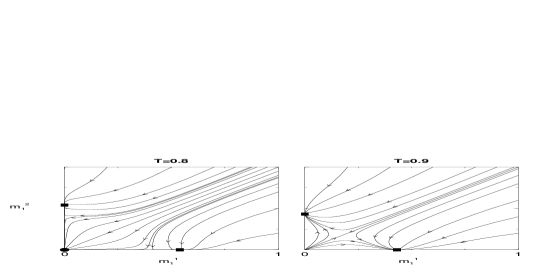
Figure 2: Flow diagrams for the model with unlinked patterns at several temperatures. Filled symbols denote different states: a circle for $0mm$, a diamond for $lmm$, a square for $mmm$ and a triangle for the symmetric state $smm$ defined in the text.

The static results found above are confirmed by a study of the dynamic behaviour of the ATNN model using the coupled eqs. (26). For simplicity, we take the number of embedded patterns of each type $p=2$. Since we have three different kinds of such patterns the results concern a six-dimensional flow. Some representative two-dimensional projections are presented in Fig. 2.

As a starting point we take ${\bf m}_{2}={\bf m}_{3}=(0.5,0)$ and different values for ${\bf m}_{1}$. Such a choice of initial conditions is not very specific because of the symmetry properties of the model. It allows us to show some typical behaviour of the network. An extensive search confirms that other initial conditions lead only to quantitatively different diagrams. We remark that the part of the diagrams not shown explicitly is symmetric with respect to the $m^{1}_{1}$ or $m^{2}_{1}$ axis. We choose some relevant values of $T$ suggested by the thermodynamics. We can locate in the first diagram of Fig. 2 ($T=0.1$) the attractor $0mm$ in the lower left corner. In the lower right (and, since there is symmetry with respect to the off-diagonal also upper left) corner we see the state $lmm$, which looks like an attractor. However, our static analysis reveals that they are only saddle points in the full six-dimensional space. On the off-diagonal we have a state of the form ${\bf m}_{1}=m_{1}(1,1)$, ${\bf m}_{2}=m_{2}(1,0)$ and ${\bf m}_{3}=m_{3}(1,0)$ denoted by $smm$, i.e., symmetric with respect to the $s$-part of the network. We remark that in this diagram some lines cross each other which is caused by the fact that only the evolution of two order parameters is shown whereas the third order parameter, $m_{2}^{1}=m_{3}^{1}$, is also evolving. One could easily imagine a three-dimensional picture with $m_{2}^{1}=m_{3}^{1}$ taken as the third coordinate.

For increasing $T$ the $smm$ state is no longer present and the $lmm$ states move along the $m_{1}^{1}$-axis (respectively $m_{1}^{2}$-axis) until they disappear for $T\approx 0.8$. For these temperatures there is a very small difference in free energy between the various Mattis-type states. This could be the reason that for $T=0.8$ we were no longer able to detect the states $lmm$ which should still exist according to the static analysis. Indeed, at this temperature the overlap for the $lmm$ states is almost equal to the one for the $mmm$ state (see Fig. 1) showing that they are almost identical. Furthermore, for $T\approx 0.8$ the states $mmm$ appear, move towards the origin on the $m_{1}^{1}$-axis (respectively the $m_{1}^{2}$-axis) as seen on the diagram for $T=0.9$ and disappear for $T=1.0$. From this temperature onwards only the origin, i.e. the $000$ state is an attractor.

4.2 Linked patterns

Next, we have analysed the model with linked patterns satisfying $\gamma^{\mu}=\xi^{\mu}\eta^{\mu}$ with $\xi$ and $\eta$ i.i.d.r.v., and with equal coupling parameters $J_{3}=J_{1}(=J_{2})=1$.

Introducing again Mattis-type states $m_{1}m_{2}m_{3}$ into the fixed-point equations (6) and checking their stability we find that there are only two stable solutions: the retrieval state $mmm$ which is stable below $T=1.213$ and the paramagnetic $000$ state which is stable above $T=1.0$. The corresponding retrieval overlap is shown in Fig. 1 (filled symbols). We notice that in contrast to the model with unlinked patterns a state of the form $mmm$ has a much bigger overlap.

Hence, we can distinguish different phases: a retrieval phase below $T=1.213$ and a paramagnetic phase above $T=1.213$. We remark that the transition at $T=1.213$ is first order. In the temperature region $1\leq T<1.213$ both the paramagnetic and Mattis solutions are local minima of the free energy. Such a region has also been seen in the Potts model but not in the Hopfield model [13]. Finally, we find that Hopfield-type solutions, i.e., Mattis states of the form $m00$ are (only) saddle points below $T=1.0$.

A detailed study of the flow equations (26) reveals a much more complicated local minima structure for this model. It turns out that for the model with linked patterns we still have to distinguish between the Mattis solutions according to the relative place of the non-zero overlap components for the different order parameters. Consequently, we introduce simple Mattis states where only the same components of the different order parameters are non-zero, e.g., ${\bf m}_{1}=m_{1}(1,0)$, ${\bf m}_{2}=m_{2}(1,0)$, and ${\bf m}_{3}=m_{3}(1,0)$ for $p=2$, denoted as before by $m_{1}m_{2}m_{3}$. For equal components $m_{\alpha}$ these are the states we have encountered in the thermodynamic analysis. (They are equivalent to $(0,m)(0,m)(0,m)$ and also to $(-m,0)(-m,0)(m,0)$).

Besides, we define crossed Mattis states where never the same components of the different order parameters are non-zero, e.g., $(m,0)(0,m)(0,0)$ for $p=2$ and $(m,0,0)(0,m,0)(0,0,m)$ for $p=3$. At this point we remark that a state of the form $(m,0)(0,m)(m,0)$ is neither simple nor crossed but of a mixed form. For $p=2$ we did not detect the latter. The crossed states are in fact equivalent to Mattis states for a model with unlinked patterns. This can easily be checked by introducing this type of solutions in the fixed-point equations for the order parameters and taking appropriate averages over the linked patterns.

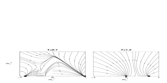
Figure 3: Flow diagrams for the model with linked patterns at different temperatures. Filled symbols stand for different states: a circle for $m00$, a square for $mmm$, a diamond for $000$ and a triangle for the asymmetric state $amm$ defined in the text.

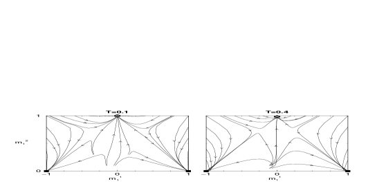
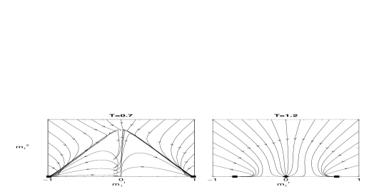
Figure 4: Flow diagrams for the model with linked patterns at different temperatures. Filled symbols stand for different states: a square for $mmm$, a diamond for $000$ and a crossed circle for $mm0$.

Some representative flow diagrams are shown in Fig. 3 and Fig. 4. As before we present only projections onto a two-dimensional space. The symmetry of the model with linked patterns is different from the model with unlinked patterns what results in a different symmetry of the flow diagrams. So, the remaining part of a diagram in these figures can be obtained by a reflection of the part displayed with respect to the axis $m_{1}^{2}=0$.

The initial conditions for the flow diagrams of Fig. 3 are as follows: two identical Mattis states with ${\bf m}_{2}={\bf m}_{3}=(0.5,0)$. We can locate in the first diagram of Fig. 3 ($T=0.1$) the attractor $mmm$ in the lower right corner. In the lower left corner we see the state $m00$, which again looks like an attractor. However, it is only a saddle point in the full six-dimensional space. On the top in the middle we have a state of the form ${\bf m}_{1}=(m_{1}^{1},m_{1}^{2})$, ${\bf m}_{2}=m_{2}(1,0)$ and ${\bf m}_{3}=m_{3}(1,0)$ denoted by $amm$, i.e., asymmetric with respect to the $s$-part of the network. We remark that also here any crossings of paths are caused by the fact that the diagrams of Fig. 3 and also of Fig. 4 are projections of a higher dimensional flow. They are not present in the full six-dimensional space.

For higher $T$ the state $amm$ disappears, the state $mmm$ stays in the lower right corner up to $T=1$ and the state $m00$ moves towards the origin and disappears at $T=1$. Above $T=1$ (see the diagram for $T=1.2$) both the origin and the state $mmm$ are stable, but the latter has already moved towards the origin. We note that in contrast with the model with unlinked patterns, it does not reach the origin since the transition (to the paramagnetic phase) is first order.

Another illustrative set of diagrams is presented in Fig. 4. Here the initial conditions are more general: ${\bf m}_{2}=(0.1,0)$, ${\bf m}_{3}=(0.5,0.0)$. In the first diagram for $T=0.1$ an attractor $mmm$ is present in the lower left and right corner. On the top in the middle the state $mm0$ is located. It is a crossed state and a minimum at low temperatures. The overlap $m$ in this state depends on $T$ in the same way as the overlap of a Mattis solution of the standard Hopfield model does.

For higher $T$ this crossed state disappears but the $mmm$ states nearly stay at the same place until $T=1$. Above, the origin is an attractor and the $mmm$ states start to move towards the origin (see the diagram for $T=1.2$). As explained above they do not reach the origin.

The interesting conclusion of these figures is that the state $mmm$ has a big basin of attraction. The latter is, of course, somewhat reduced in the temperature region where also the stable state $000$ appears. Furthermore, the state $mmm$ has a large overlap (recall Fig. 1) with the embedded patterns.

Since the ATNN model with linked patterns seems to have very good retrieval properties it is worthwhile to derive a $\beta J_{1}-\beta J_{3}$ phase diagram. We first note that the fixed-point equations (6) for the simple Mattis states have the same form as those for the mean-field Ashkin-Teller model. Because these states are always the global minima of the free energy they determine the transition lines. Of course the meaning of the phases is different from the standard Ashkin-Teller model. For the special case of one embedded pattern, i.e., $p=1$, with $\xi_{i}^{1}=\eta_{i}^{1}=1$ both models are completely equivalent.

The ATNN $\beta J_{1}-\beta J_{3}$ phase diagram (for low loading of linked patterns) is presented in Fig. 5. We distinguish the following phases. The area in dark grey is the paramagnetic $000$ phase. The light shadowed area is the full retrieval phase (for linked patterns) described by the simple Mattis state $mml$ ($m\neq l$ when $J_{1}\neq J_{3}$). The white area represents a partial retrieval phase, i.e., only patterns embedded in one part of the network are recalled by the state $00l$. The (thick) full lines indicate second order transitions, the (thick) dashed lines discontinuous ones. We remark that the $000$ state exists as a minimum up to the thin full lines, but outside the dark grey region its energy is higher than the energy of the $mml$ state. In part of the full retrieval phase, namely in the upper half of the phase diagram, the crossed state $mm0$ exists. It is stable in the area above the thin full and thin dashed lines.

5 Conclusions

We have analysed a neural network version of the Ashkin-Teller spin-glass model for low loading of patterns. Both the thermodynamic and dynamic properties have been considered, especially for Mattis states which are the most interesting states from the point of view of retrieval. Fixed-point equations as well as flow equations for the relevant order parameters have been derived. Numerical results have been discussed illustrating the typical behaviour of the network.

The following main conclusions can be drawn. For unlinked embedded patterns the behaviour of the model is much richer than in the case of the standard Hopfield model in the sense that many different forms of stable Mattis states are possible. These states exist up to $T=1$ where a continuous transition occurs from the retrieval phase to the paramagnetic phase. The corresponding flow diagrams are quite complicated but verify the existence of these many attractors. However, none of these retrieval states has a bigger overlap than the Mattis states of a corresponding Hopfield model. Hence the inclusion of the four-neuron interaction term does not particularly improve the quality of retrieval.

For linked embedded patters interesting new features show up. The most important one is that stable Mattis states of the form $mmm$ appear. They have a very big overlap with the embedded patterns, meaning that the pairs of patterns which are linked by the four-neuron term are retrieved with a very high accuracy. Furthermore, they exist up to $T=1.213$ and have a big basin of attraction. For temperatures $1\leq T\leq 1.213$ both these Mattis states and the paramagnetic solution are local minima of the free energy such that their basin of attraction is somewhat reduced. To verify then that this big overlap $m$ is not just a rescaled overlap of the corresponding Mattis state of a corresponding Hopfield model we have made a comparison in Fig. 6. We clearly see the difference in shape in favour of the ATNN. Further details of additional features of the ATNN model are given in a $\beta J_{1}-\beta J_{3}$ phase diagram (see Fig. 5). In brief, the linked pairs are retrieved easily and with a high precision (simple states) and the unlinked pairs may be retrieved (crossed states), but always with lower precision than that of the linked ones. It is important to stress that the patterns which are linked can be completely different. In principle, they are independent.

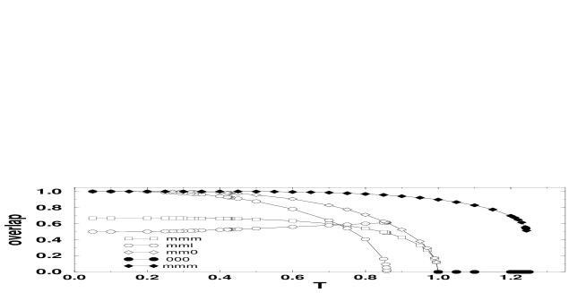
Figure 1: The overlaps for the Mattis states as a function of the temperature $T=1/\beta$ for $J_{1}=J_{2}=J_{3}=1$. States represented by filled symbols are only present for the model with linked patterns.

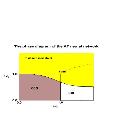
Figure 5: The $\beta J_{1}-\beta J_{3}$ phase diagram of the ATNN model with linked patterns. The dark grey area represents the $000$ phase, the light grey area the full retrieval phase $mml$ and the white area the partial retrieval phase $00l$. Thick full lines indicate continuous transitions, thick dashed lines discontinuous ones.

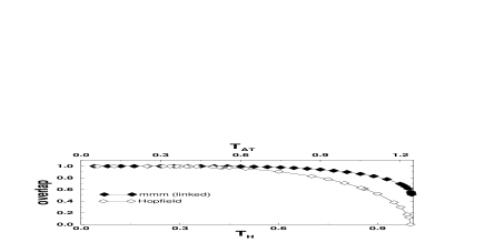
Figure 6: The overlap as a function of a rescaled $T$ for the state $mmm$ in the ATNN model with linked patterns (filled diamond) versus the overlap for the Mattis state in the Hopfield model (empty diamond). Respective temperatures are denoted by $T_{AT}$ and $T_{H}$.

References

- [1] Hopfield J J 1982 Proc. Nat. Acad. Sci. USA 79 2554
- [2] Gerl F and Krey U 1994 J. Phys. A: Math. Gen. 27 7353
- [3] Bollé D, van Hemmen J L and Huyghebaert J 1996 Phys. Rev. E 53 1276
- [4] Kühn R and Bös S 1993 J. Phys. A: Math. Gen. 26 831
- [5] Bollé D, Rieger H and Shim G M 1994 J. Phys. A: Math. Gen. 27 3441
- [6] Christiano P L and Goulart Rosa Jr S 1986 Phys. Rev. A 34 730
- [7] Moreira J V and Christiano P L 1992 Phys. Lett. A 162 149
- [8] Moreira J V and Christiano P L 1992 J. Phys. A 25 L739
- [9] Nobre F D and Sherrington D 1993 J.Phys A 26 4539
- [10] Viana L and Martinez C 1995 J. Phys. I France 5 573
- [11] Provost J P and Vallee G 1982 Phys.Rev.Lett. 49 409
- [12] Amit D J, Gutfreund H and Sompolinsky H 1985 Phys. Rev. A 32 1007
- [13] Bollé D and Mallezie F 1989 J.Phys A 22 4409
- [14] van Hemmen J L, Grensing D, Huber A and Kühn R 1986 Z. Phys. B 65 53
- [15] Coolen A C C and Ruijgrok TH W 1988 Phys .Rev. A 38 4253