Localization in non-Hermitian quantum mechanics
and flux-line pinning in superconductors

Abstract

A recent development in studies of random non-Hermitian quantum systems is reviewed. Delocalization was found to occur under a sufficiently large constant imaginary vector potential even in one and two dimensions. The phenomenon has a physical realization as flux-line depinning in type-II superconductors. Relations between the delocalization transition and the complex energy spectrum of the non-Hermitian systems are described. Analytical and numerical results obtained for a non-Hermitian Anderson model are shown.

1 Introduction

The main purpose of the present paper is to review a new development in studies of non-Hermite operators. The review is mostly based on the work by the present author in collaboration with Nelson [1, 2] and the works following it [3, 4, 5, 6, 7, 8, 9, 10, 11, 12, 13, 14]. In addition, I report a new numerical result for a non-Hermitian ladder system.

Non-Hermite operators appear frequently in dynamical systems as Liouville operators. Although less frequently, they also appear in the context of quantum mechanics as Hamiltonian operators in the Schrödinger equation. A well-known example is the optical potential, which is a complex scalar potential that effectively describes multiple scattering and absorption. A non-Hermite Hamiltonian can also emerge when one relates a $(d+1)$-dimensional classical statistical system to a $d$-dimensional quantum system by path-integral scheme or the Suzuki-Trotter transformation [15]. As a classic example, McCoy and Wu [16] showed that equilibrium classical statistical mechanics of a two-dimensional asymmetric vertex model can be described by imaginary-time quantum dynamics of a non-Hermitian $XXZ$ spin chain. In this case, the non-Hermiticity of the spin chain is originated in an external field that generates a diagonal flow of edge spins of the vertex model.

The new development reviewed here resulted from introduction of quenched randomness into non-Hermitian quantum systems. A delocalization phenomenon was found for an especially simple class of random non-Hermite Hamiltonians even in one and two dimensions. The Hamiltonian contains a constant imaginary vector potential and a real random scalar potential. As the imaginary vector potential increases, all of originally localized eigenfunctions get delocalized one by one. One of the remarkable features is that a complex eigenvalue of the Hamiltonian indicates the delocalization of the corresponding eigenfunction. Thus we can study the delocalization phenomenon simply by investigating the energy spectrum of the non-Hermite Hamiltonian.

The delocalization phenomenon has a physical realization as flux-line depinning in type-II superconductors. Basic correspondence between the delocalization and the depinning is described in the next section. In Section 3, I discuss the complex-energy spectrum of the random non-Hermitian system, using numerical data for a non-Hermitian Anderson model. A new result for a non-Hermitian ladder system is also reported. Section 4 presents an interesting application of Mott’s variable-range hopping to the non-Hermitian quantum mechanics.

Non-Hermite matrices with randomness have recently attracted much attention from other viewpoints as well. The spectrum of the Fokker-Planck operator with a random velocity field has been studied in Refs. [17, 18]. Non-Hermitian random matrix theory has seen great progress recently [5, 13, 19, 20, 21, 22, 23, 24, 25, 26]. The present review, however, does not cover these topics.

2 Non-Hermitian quantum mechanics and flux lines in superconductors

2.1 Random non-Hermite Hamiltonian and an elastic string in a random washboard potential

A typical Hamiltonian which I treat here is

$${\cal H}\equiv\frac{(\vec{p}+\mathrm{i}\vec{g})^{2}}{2m}+V(\vec{x}),$$ (1)

where $\vec{p}=(\hbar/\mathrm{i})\partial/\partial\vec{x}$ is the momentum operator, $\vec{g}$ is a constant real vector referred to as a non-Hermitian field, and $V$ is a random potential. A lattice version of the above Hamiltonian is given by a non-Hermitian Anderson model on a hypercubic lattice,

$${\cal H}\equiv\sum_{\vec{x}}\left[-\frac{t}{2}\sum_{\nu=1}^{d}\left(\e^{\vec{g}\cdot\vec{e}_{\nu}/\hbar}\Bigl{|}\vec{x}+\vec{e}_{\nu}\Bigr{\rangle}\Bigl{\langle}\vec{x}\Bigr{|}+\e^{-\vec{g}\cdot\vec{e}_{\nu}/\hbar}\Bigl{|}\vec{x}\Bigr{\rangle}\Bigl{\langle}\vec{x}+\vec{e}_{\nu}\Bigr{|}\right)+V_{\vec{x}}\Bigl{|}\vec{x}\Bigr{\rangle}\Bigl{\langle}\vec{x}\Bigr{|}\right],$$ (2)

where $t$ is the hopping amplitude, the vectors $\{\vec{e}_{\nu}\}$ are the unit lattice vectors, and $V_{\vec{x}}$ is an on-site random potential following a probability distribution $P(V_{\vec{x}})$. Periodic boundary conditions are applied to wave functions in both cases. Note that the non-Hermitian field $\vec{g}$ plays a role of an imaginary vector potential.

In the Hermitian case $\vec{g}=\vec{0}$, Eqs. (1) and (2) are reduced to the standard Hamiltonians for the Anderson localization. It is widely accepted for $\vec{g}=\vec{0}$ that all eigenfunctions are localized in one and two dimensions. The present author and Nelson recently found [1, 2] that all of the localized eigenfunctions get delocalized one by one as the non-Hermitian field $\vec{g}$ is increased and that appearance of complex eigenvalues indicates the delocalization transition.

As is exemplified in the study of McCoy and Wu [16], a non-Hermite Hamiltonian can have physical relevance when it is mapped to a classical statistical-mechanical system with path-integral mapping. By identifying the imaginary-time-evolution operator $\e^{-\Delta\tau{\cal H}}$ of the Hamiltonian (1) as the transfer matrix of a classical system, we can transform [27, 28] the matrix element of the time-evolution operator between the initial and final vectors,

$${\cal Z}\equiv\left\langle\psi^{\mathrm{f}}\Bigm{|}\e^{-L_{\tau}{\cal H}/\hbar}\Bigm{|}\psi^{\mathrm{i}}\right\rangle,$$ (3)

into the partition function of an elastic string in a $(d+1)$-dimensional space,

$${\cal Z}=\int{\cal D}\vec{x}\e^{-{E_{\mathrm{cl}}[\vec{x}(\tau)]}/\hbar}$$ (4)

with the energy of the string given by

$$E_{\mathrm{cl}}[\vec{x}(\tau)]\equiv\int_{0}^{L_{\tau}}\d\tau\left[\frac{m}{2}\left(\frac{\d\vec{x}}{\d\tau}\right)^{2}-\vec{g}\cdot\frac{\d\vec{x}}{\d\tau}+V(\vec{x})\right].$$ (5)

The first term of the energy describes the elasticity of the string. (See Appendix for details of the above transformation.)

The energy (5) of the elastic string is re-interpretation of the imaginary-time action of the quantum particle. The imaginary-time axis $\tau$ of the quantum system is identified as an additional spatial axis of the classical system. Hence the imaginary time $L_{\tau}$ becomes the system size of the classical system in the $\tau$ direction. The world line of the quantum particle, $\vec{x}(\tau)$, is identified as a spatial configuration of the classical elastic string subject to thermal fluctuations. The temperature of the classical system is given by the Planck parameter $\hbar$. The integral $\int{\cal D}\vec{x}$ denotes the summation over all possible configurations of the world line, or the elastic string.

Note that the random potential does not depend on $\tau$. Hence the elastic string is put on a “random washboard” potential (Fig. 1).

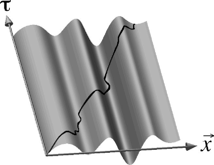
Figure 1: An elastic string in a random washboard potential is subject to thermal fluctuations. The energy of the string is given by Eq. (5). Through path-integral mapping, statistical mechanics of the system is equivalent to quantum dynamics of the Hamiltonian (1).

The potential tries to trap the elastic string in particularly deep valleys and thereby to align the string along the $\tau$ direction. On the other hand, the second term of the energy (5), which comes from the non-Hermitian field $\vec{g}$, tries to tilt the string away from the $\tau$ direction as is explained below. (In fact, if the random potential is not present, the energy is optimized when the string is tilted by the angle $\tan^{-1}(g/m)$.) The competition between the above two effects results in a pinning-depinning transition of the string from the random washboard potential. This in turn indicates a localization-delocalization transition of the quantum particle subject to the non-Hermitian field and the random potential.

The reason why the non-Hermitian field $\vec{g}$ in the quantum system has the effect of tilting the elastic string may be explained in the following way. A vector potential $\vec{A}$ generally induces a current in a quantum system because of the coupling $\vec{p}\cdot\vec{A}$ in the Hamiltonian. The current would be expressed by the world lines of quantum particles running diagonally in the real-time-space. Since the present non-Hermitian field plays a role of an imaginary vector potential, it induces an imaginary current. The imaginary current is expressed by tilted world lines in the imaginary-time-space. Hence the field $\vec{g}$ tries to tilt the world line, or the elastic string.

2.2 Flux-line pinning in type-II superconductors

The situation described by Eq. (5) is realized in type-II superconductors with extended defects. In a harmonic approximation, Nelson and Vinokur [29] derived a phenomenological Hamiltonian of a flux line in a superconductor with extended defects. The Hamiltonian takes the form of Eq. (5) with $V(\vec{x})$ denoting the pinning potential due to the defects.

When an electric current is applied to a pure sample of a type-II superconductor in the mixed phase, magnetic flux lines penetrating the sample are moved by electromagnetic forces, dissipate energy, and thus destroy the superconductivity. Randomly located (but mutually parallel) extended defects such as columnar defects (typically created by bombardment of heavy ions) and twin boundaries (planer defects in the anisotropic YBCO) pin the flux lines efficiently as long as the flux lines are almost parallel to the defects [29, 30, 31]. When the external magnetic field is tilted away from the defects, but its transverse component $\vec{H}_{\perp}$ is still small, we may expect that the bulk part of the flux line remains pinned (Fig. 2(a)).

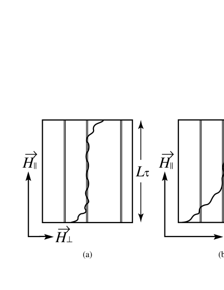
Figure 2: Flux-line depinning due to tilt of the external magnetic field. (a) When the transverse component of the magnetic field is small, the flux line is pinned by a columnar defect in the bulk of the superconductor, although it is deflected near the surfaces. (b) For a larger $\vec{H}_{\perp}$, the flux line is depinned from the defect.

This is referred to as the transverse Meissner effect [29], because the system in this region exhibits perfect bulk diamagnetism in the transverse direction. When one increases the tilt angle (Fig. 2(b)), a depinning transition occurs at a certain strength of the transverse magnetic field, namely $H_{\perp\mathrm{c}}$. (See Section 4 for further details.)

The above depinning transition can be explained in a clear-cut way in terms of delocalization in the random non-Hermitian quantum mechanics [1, 2]. The depinning of the flux line corresponds to delocalization of the relevant wave function of the quantum system; see Table 1 for other correspondence.

Table 1: Correspondence between the random non-Hermitian system and the flux-line system.

Random non-Hermitian system	Flux-line system
$d$-dimensional space	$(d+1)$-dimensional space
and the imaginary time
Quantum fluctuation	Thermal fluctuation
World line	Flux line
Non-Hermitian field $\vec{g}$	Transverse field $\vec{H}_{\perp}$
Random potential $V(\vec{x})$	Randomly located extended defects
Localization	Pinning
Delocalization	Depinning
Real eigenvalue	Transverse Meissner effect
Complex eigenvalue in a periodic system	Helical structure of a flux line
Imaginary current of a quantum particle	Tilt of a flux line

Although it would be possible to describe the depinning within the framework of classical statistical mechanics, one can take advantage, in the non-Hermitian approach, of abundant results available concerning localization in Hermitian random systems. It is also often practically easier to solve a Schrödinger equation than to treat the same problem in the path-integral framework.

There are many other physical realizations of the above random non-Hermitian system. Efetov [4] discussed the problem from the viewpoint of directed quantum chaos. Nelson and Shnerb found an interesting application to population biology [11]. In an independent work, Chen et al. [32] employed the same technique to study sliding of charge-density waves in disordered systems. In the following, I concentrate on the flux-line analogy.

3 Complex eigenvalues and delocalization

3.1 Energy spectrum in one dimension

I now present an example of the energy spectrum of the random non-Hermitian system [1, 2]. Figure 3 shows numerical results for the lattice Hamiltonian (2) in one dimension with 1000 sites.

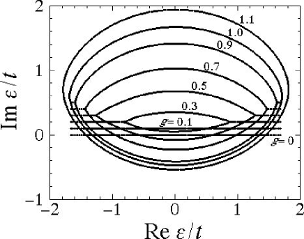
Figure 3: The energy spectrum of the one-dimensional non-Hermitian model (2) with 1000 sites. Each eigenstate $\varepsilon$ is marked by a tiny cross in the complex energy plane. Plots for different values of $g$ are offset for clarity. The random potential at each site was chosen from a box distribution over the range $[-t,t]$. The same realization of the random potential $\{V_{x}\}$ was used for all plots here. A complex eigenvalue indicates that the eigenstate is delocalized and the corresponding flux line is depinned.

All energy eigenvalues are of course real for the Hermitian case $g=0$. For weak $g$, e.g. $g/\hbar=0.1$ in the case of Fig. 3, all the eigenvalues are still real despite the fact that the Hamiltonian is non-Hermite. As we increase $g$, complex eigenvalues appear in the middle of the energy band and form a bubble. (The spectrum has an inversion symmetry with respect to the real energy axis, because the Hamiltonian (2) is a real matrix.) The region of complex eigenvalues expands towards the band edges as $g$ is increased, and the whole spectrum eventually becomes almost elliptic. In fact, the spectrum exactly falls onto an ellipse if $V_{x}\equiv 0$ [1, 2]:

$$\left(\frac{\mathop{\mathrm{Re}}\varepsilon}{\cosh(g/\hbar)}\right)^{2}+\left(\frac{\mathop{\mathrm{Im}}\varepsilon}{\sinh(g/\hbar)}\right)^{2}=t^{2}.$$ (6)

Analytic forms of the random-averaged energy spectrum in one dimension have been obtained for weak disorder and weak $g$ [7] and for general values of $g$ with the Lorentzian random distribution [9, 10]. By neglecting higher moments of the random distribution of the on-site potential $\{V_{x}\}$, Brouwer et al. obtained an approximate shape of the bubble after averaging, in the form

$$|\mathop{\mathrm{Im}}\varepsilon|=\frac{|g|}{\hbar}\sqrt{t^{2}-(\mathop{\mathrm{Re}}\varepsilon)^{2}}-\frac{\Delta^{2}}{2\sqrt{t^{2}-(\mathop{\mathrm{Re}}\varepsilon)^{2}}}$$ (7)

for $|\mathop{\mathrm{Re}}\varepsilon|<\varepsilon_{\mathrm{c}}$ and for small $|g|$, where $\Delta^{2}\equiv\langle V_{x}^{2}\rangle$ is the second moment of the random distribution and

$$\varepsilon_{\mathrm{c}}\equiv\sqrt{t^{2}-\frac{\hbar\Delta^{2}}{2|g|}}.$$ (8)

The value of $\varepsilon_{\mathrm{c}}$ indicates the region of the bubble of complex eigenvalues and in fact is a “mobility edge” as discussed below. Note that the bubble does not exist for $|g|<\hbar\Delta^{2}/(2t^{2})$.

For the Lorentzian distribution of the potential, $P(V_{x})=\pi^{-1}\gamma/(V_{x}^{2}+\gamma^{2})$, whose second moment is diverging, the exact shape of the bubble after averaging was obtained for general values of $g$ [9, 10]:

$$\left(\frac{\mathop{\mathrm{Re}}\varepsilon}{\cosh(g/\hbar)}\right)^{2}+\left(\frac{|\mathop{\mathrm{Im}}\varepsilon|+\gamma}{\sinh(g/\hbar)}\right)^{2}=t^{2}$$ (9)

for $|\mathop{\mathrm{Re}}\varepsilon|<\varepsilon_{\mathrm{c}}$ with the “mobility edge”

$$\varepsilon_{\mathrm{c}}\equiv\cosh(g/\hbar)\sqrt{t^{2}-\gamma^{2}{\mathop{\mathrm{sech}}}^{2}(g/\hbar)}.$$ (10)

The form (9) is remarkably simple; the upper and lower halves of the elliptic spectrum of the pure case, Eq. (6), are squeezed towards the real energy axis translationally by the distance $\gamma$, preserving the shape of the arcs. Eigenvalues that lost the support of the arcs become real and are distributed over the whole real axis except for the region of the bubble. The bubble entirely vanishes for $|g|<\hbar\sinh^{-1}(\gamma/t)$.

Another approximate expression of the mobility edge $\varepsilon_{\mathrm{c}}$ has been obtained for general random distribution [6, 13]. For the Lorentzian randomness, this expression is reduced to the exact result (10).

3.2 Delocalization and complex eigenvalues

In the following, I explain the correspondence that is listed in Table 2.

Table 2: The delocalization criterion of the random non-Hermitian system. A wave function of the form $\psi\sim\e^{-\kappa|\vec{x}|}$ for $\vec{g}=\vec{0}$ and $|\vec{x}|\to\infty$ gets delocalized when $|\vec{g}|$ exceeds $\hbar\kappa$, and acquires a complex eigenvalue at the same time.

non-Hermitian field $\vec{g}$	wave function	eigenvalue
$|\vec{g}|<\hbar\kappa$	localized	real
$|\vec{g}|>\hbar\kappa$	delocalized	complex

I first argue that a complex eigenvalue indicates a delocalized wave function. Consider the imaginary-time dynamics of a wave function

$$\psi(\vec{x};\tau)=\psi(\vec{x})\e^{-\tau\varepsilon}\propto\e^{-\mathrm{i}\tau\mathop{\mathrm{Im}}\varepsilon},$$ (11)

where $\varepsilon$ is the eigenvalue of the eigenfunction $\psi(\vec{x})$. The above equation shows that the imaginary part of the eigenvalue, if it exists, gives rise to an oscillatory behavior of the system in the imaginary-time direction. In fact, the oscillatory behavior comes from the world line wrapping around the system as a helix (Fig. 4).

Figure 4: The world line (the thick line) of a current-carrying particle forms a helix when periodic boundary conditions are imposed in the space direction. Hence periodicity appears in the imaginary-time direction. The periodicity is described by an oscillatory factor $\e^{\mathrm{i}\tau\mathop{\mathrm{Im}}\varepsilon}$.

Note here that periodic boundary conditions in the space directions are imposed on the quantum system. Hence a quantum particle, when it is delocalized, circulates around the system. This yields a helical flow ascending in the imaginary-time direction of the $(d+1)$-dimensional imaginary-time-space. The pitch of the helix corresponds to the reciprocal of the imaginary part of the energy.

It follows from the above argument that a wave function of the periodic system acquires a complex eigenvalue as soon as it gets delocalized, or the corresponding flux line gets depinned and tilted. Thus observing the energy spectrum of the non-Hermite Hamiltonian is a convenient way of investigating the flux-line depinning.

Next, I explain the delocalization criterion $|\vec{g}|\mathchoice{\mathrel{\vbox{\hbox{$\buildrel\displaystyle<\over{\displaystyle>}$}}}}{\mathrel{\vbox{\hbox{$\buildrel\textstyle<\over{\textstyle>}$}}}}{\mathrel{\vbox{\hbox{$\buildrel\scriptstyle<\over{\scriptstyle>}$}}}}{\mathrel{\vbox{\hbox{$\buildrel\scriptscriptstyle<\over{\scriptscriptstyle>}$}}}}\hbar\kappa$ in Table 2. For this purpose, I introduce the imaginary gauge transformation [33]. Suppose that we obtain an eigenfunction of the Hamiltonian for $\vec{g}=\vec{0}$ with a real energy eigenvalue:

$${\cal H}_{0}\psi_{0}(\vec{x})=\varepsilon_{0}\psi_{0}(\vec{x}).$$ (12)

Since the non-Hermitian field $\vec{g}$ is equivalent to an imaginary vector potential, we may be able to gauge out the field from the non-Hermite Hamiltonian ${\cal H}(\vec{g})$. In other words, the eigenfunction of the Hamiltonian ${\cal H}(\vec{g})$ corresponding to $\psi_{0}$ may be given by

$$\psi(\vec{x})=\e^{\vec{g}\cdot\vec{x}/\hbar}\psi_{0}(\vec{x})$$ (13)

and the eigenvalue $\varepsilon_{0}$ may remain the same.

The above transformation is valid only in a certain range of $\vec{g}$. Assume that the wave function for $\vec{g}=\vec{0}$ is asymptotically given by $\psi_{0}(\vec{x})\sim\e^{-\kappa|\vec{x}|}$, where $\kappa$ is a constant. Equation (13) then takes the form

$$\psi(\vec{x})\sim\e^{-\kappa|\vec{x}|+\vec{g}\cdot\vec{x}/\hbar}.$$ (14)

This wave function is (asymmetrically) localized for $|\vec{g}|<\hbar\kappa$. In this region the function (14) satisfies periodic boundary conditions asymptotically in the infinite-system-size limit. Hence the imaginary gauge transformation is valid for $|\vec{g}|<\hbar\kappa$ and Eq. (13) is indeed the eigenfunction of the non-Hermite Hamiltonian ${\cal H}(\vec{g})$ with the real eigenvalue $\varepsilon_{0}$. In fact, closer inspection of the spectrum in Fig. 3 would reveal that the real eigenvalues in the “wings” of the spectrum does not depend on $g$. This rigidity reflects the transverse Meissner effect of the corresponding flux-line system.

For $|\vec{g}|>\hbar\kappa$, on the other hand, the function (14) does not satisfy periodic boundary conditions, because it blows up in the direction of $\vec{g}$ in this region. Thus Eq. (13) is no longer an eigenfunction of the non-Hermite Hamiltonian ${\cal H}(\vec{g})$. It is in this region that the eigenfunction is delocalized and acquires a complex eigenvalue. (Equation (13) is an eigenfunction if we impose open boundary conditions. All the eigenvalues remain real in this case, although the eigenfunctions are nonetheless delocalized. This is consistent with the fact that the helix in Fig. 4 never appears if the boundaries are open in the spatial directions.)

3.3 Mobility edge and inverse localization length

According to the above argument, the eigenstates that belong to the bubble in Fig. 3 are delocalized, while those in the wings of the real eigenvalues are localized. Hence the two vertices of the bubble, $\varepsilon_{\mathrm{c}}$ and $-\varepsilon_{\mathrm{c}}$, are mobility edges. The complex energy eigenvalues appear first in the middle of the energy band because, in the one-dimensional Anderson model ($g=0$), $\kappa$ is the smallest for the eigenstate at $\varepsilon=0$, as exemplified below.

Table 2 provides a convenient method of estimating the inverse localization length for $g=0$. It is deduced from the delocalization criterion that a state at a mobility edge for a value $g_{0}$ of the non-Hermitian field has the inverse localization length $\kappa=|g_{0}|/\hbar$ for $g=0$. A numerical calculation of $\kappa$ by this method was presented in Ref. [2] for the one-dimensional lattice model with a box distribution. Using the analytic result (10), we can also calculate the inverse localization length of the Lloyd model [34] (the one-dimensional Anderson model ($g=0$) with the Lorentzian random distribution) as a function of the energy, by solving

$$\varepsilon=\cosh\kappa\sqrt{t^{2}-\gamma^{2}{\mathop{\mathrm{sech}}}^{2}\kappa},\qquad\mbox{or}\qquad\left(\frac{\varepsilon}{\cosh\kappa}\right)^{2}+\left(\frac{\gamma}{\sinh\kappa}\right)^{2}=t^{2}.$$ (15)

The solution

$$\kappa(\varepsilon)=\cosh^{-1}\frac{\displaystyle\sqrt{(\varepsilon+t)^{2}+\gamma^{2}}+\sqrt{(\varepsilon-t)^{2}+\gamma^{2}}}{2t}$$ (16)

reproduces the exact result obtained by Hirota and Ishii [35, 36] and Thouless [37].

Figure 5 shows the function $\kappa(\varepsilon)$ for $t=\gamma=1$.

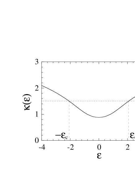
Figure 5: The inverse localization length (16) of the Lloyd model (the solid line). The parameter values used in this figure are $t=\gamma=1$. The crossing points of the solid line and the dotted line (indicating a value of $g/\hbar$) yield the mobility edges $\varepsilon_{\mathrm{c}}$ and $-\varepsilon_{\mathrm{c}}$.

If we apply to the system the non-Hermitian field of the value, say, $g/\hbar=1.5$ as indicated by a dotted line in Fig. 5, the eigenstates below the dotted line ($-\varepsilon_{\mathrm{c}}<\varepsilon<\varepsilon_{\mathrm{c}}$) get delocalized and form a bubble in the spectrum, while those above the line ($\varepsilon<-\varepsilon_{\mathrm{c}}$ and $\varepsilon>\varepsilon_{\mathrm{c}}$) remain localized and stay in the wings of the spectrum.

3.4 Other one-dimensional models

Feinberg and Zee [8, 12] introduced an interesting limit of the lattice Hamiltonian (2) in one dimension, namely the one-way model:

$${\cal H}\equiv\sum_{x}\left(-\left|x+1\right\rangle\left\langle x\right|+V_{x}\left|x\right\rangle\left\langle x\right|\right).$$ (17)

In other words, they took an extremely non-Hermitian limit, $t\e^{g/\hbar}\to 2$ and $t\e^{-g/\hbar}\to 0$. Exact calculations of the spectral curve $(\mathop{\mathrm{Re}}\varepsilon,\mathop{\mathrm{Im}}\varepsilon)$ and the mobility edge $\varepsilon_{\mathrm{c}}$ become possible for various random distributions including the box distribution, the binary distribution and even diluted randomness. See Ref. [12] for details.

In Figure 6, I show a numerical result of the energy spectrum of a ladder system,

(a)

(b)

(c)

(d)

Figure 6: The energy spectrum of the non-Hermitian ladder model (18) with 500$\times$2 sites. Each eigenstate $\varepsilon$ is marked by a tiny cross in the complex energy plane. The random potential at each site was chosen from a box distribution over the range $[-t,t]$. The same realization of the random potential $\{V_{x}\}$ was used for all plots here: (a) $g/\hbar=0.3$, (b) $g/\hbar=0.5$, (c) $g/\hbar=0.7$ and (d) $g/\hbar=0.9$.

$${\cal H}\equiv{\cal H}_{1}+{\cal H}_{2}-\frac{t}{2}\sum_{x}\left(\left|x,2\right\rangle\left\langle x,1\right|+\left|x,1\right\rangle\left\langle x,2\right|\right),$$ (18)

where ${\cal H}_{1}$ and ${\cal H}_{2}$ is the non-Hermitian Anderson Hamiltonian for each leg of the ladder while the last term denotes hopping between the legs; “$x,1$” and “$x,2$” denote a site on the first and second leg, respectively. Alternatively we may regard the labels 1 and 2 as an additional degree of freedom such as spin or flavor. On the basis of the argument in the previous subsection, we can deduce from the result in Fig. 6 that there are two minima of $\kappa(\varepsilon)$ in the Hermitian ladder system.

The above numerical calculation was immediately followed by Zee’s analytic calculation of the spectrum for the Lorentzian randomness [14]. Just as in the one-dimensional case (10), the averaged spectrum is squeezed towards the real axis as the randomness is increased. Thereby we can exactly calculate $\kappa(\varepsilon)$ for the ladder Lloyd model. The result is simply superposition of two functions of the form (16). This is consistent with the above numerical result for the box distribution.

Note that, except in the case of the single chain, $\kappa(\varepsilon)$ thus calculated is an upper bound of what is referred to as the “inverse localization length” in the context of the Anderson localization [38, 39, 40]. The geometric average of the Green’s function is taken in defining the Anderson-localization length, while the arithmetic average is taken in the above analytic calculation. (The argument that yielded Table 2 is still valid for each realization of the random potential.)

3.5 Energy spectrum in two dimension

Finite-size calculations of the energy spectrum of the non-Hermite Hamiltonian (2) for $d=2$ [1, 2] appeared to suggest the following three regions of the non-Hermitian field $\vec{g}$. First, it is widely accepted for $\vec{g}=\vec{0}$ that all eigenstates of two-dimensional random systems are localized with finite localization lengths. Hence, by using the imaginary gauge transformation again, we can conclude that there is a finite region of small $\vec{g}$ where all states remain localized. This is consistent with the finite-size data [1, 2]. As $\vec{g}$ is increased, delocalized states with complex eigenvalues appear as in the one-dimensional case. For intermediate values of $\vec{g}$, however, the energy spectrum shows much more complicated structure than in the one-dimensional case; see Ref. [2] for details. For larger $\vec{g}$, the spectrum becomes similar to the one of the system without impurities, as was the case in $d=1$.

Nelson and Shnerb [11] suggested that the third region of $\vec{g}$ disappears in the thermodynamic limit. For a very large $\vec{g}$, or a very large transverse magnetic field $\vec{H}_{\perp}$, the flux line lies nearly sideways in the superconductor. When we project the flux line and the columnar defects onto a two-dimensional plane from above, the problem is approximately reduced to a string lying on a plane with point impurities. Nelson and Shnerb analyzed this reduced problem in terms of Burger’s equation with noise [41] (or the Kardar-Parisi-Zhang equation [42]) and predicted a fractal geometry of the flux-line configuration. This fractality may cause the complicated energy spectrum observed in the second region of $\vec{g}$. The fractal geometry does not emerge until the system size becomes larger than a certain crossover length, which can explain the appearance of the third region of $\vec{g}$ in the finite-size data [1, 2]. The above theoretical prediction is consistent with numerical results in Ref. [32], although the numerical estimate of the exponent characterizing the fractal geometry is somewhat different from the theoretical value predicted by Nelson and Shnerb [11].

Note, however, that a different conclusion may be suggested by Zee’s analytic calculation of the two-dimensional spectrum for the Lorentzian random potential [14]. In the case of the Lorentzian random distribution, just as in one dimension, the averaged spectrum is squeezed towards the real axis as the randomness is increased. In the process, the spectrum keeps the regular structure of the spectrum of the non-random system.

4 Transverse Meissner effect

One of the interesting issues in the context of the flux-line depinning is how the transverse Meissner effect breaks down as the depinning point is approached from the side of the pinning phase. As is shown schematically in Fig. 2, the pinning breaks first near the surface. This is also observed in numerical results [2]. Thus we can define a penetration depth $\tau^{\ast}$ for the transverse Meissner effect as the typical thickness of the sub-surface region where the flux line is deflected from the pinning center. (Note that $\tau^{\ast}$ is different from the penetration depth of the underlying superconductivity.) The penetration depth $\tau^{\ast}$ diverges with a certain exponent, as we increase $\vec{H}_{\perp}$, or $\vec{g}$. This divergence leads to the breakdown of the bulk pinning. The conclusion of Refs. [1, 2] is

$$\tau^{\ast}\sim(H_{\perp\mathrm{c}}-H_{\perp})^{-d},$$ (19)

where $H_{\perp\mathrm{c}}$ is the depinning field. Note that the dimensionality of the superconductor is $d+1$.

Since we regard the flux line as the world line of a quantum particle in the framework of the non-Hermitian quantum mechanics, the deflection of the flux line is interpreted as hopping of the quantum particle from a strong impurity (the localization center) to weaker impurities. Near the delocalization point $g_{\mathrm{c}}$($\propto H_{\perp\mathrm{c}}$), Mott’s argument of variable-range hopping [43] is readily applicable even to the non-Hermitian case. Minimizing a hopping matrix element near the surface leads to Eq. (19).

5 Summary

A class of random non-Hermitian quantum systems has been found to be relevant to various physical systems and to show intriguing properties. In particular, the delocalization phenomenon of the random non-Hermitian system is equivalent to the depinning of a flux line in type-II superconductors. We can investigate the delocalization just by observing the energy spectrum of the non-Hermite Hamiltonian. Various depinning phenomena may be understood in a similar way. Interesting future problems include many-band non-Hermitian Anderson models, detection of the fractality in the spectrum of the two-dimensional system, and generalization of the theory to the case of interacting systems.

Appendix A Path-integral mapping

I here show derivation of Eq. (4) from Eq. (3). There are various ways of formulating the path-integral mapping. The following is based on the formulation in Ref. [28], which employs the Trotter decomposition [15]:

$$\e^{-L_{\tau}{\cal H}/\hbar}=\lim_{n\to\infty}\left(\e^{-{\cal V}\Delta\tau/\hbar}\e^{-{\cal K}\Delta\tau/\hbar}\right)^{n}.$$ (20)

Here ${\cal K}$ and ${\cal V}$ denote the kinetic and potential terms of the Hamiltonian (1), respectively, and $\Delta\tau\equiv L_{\tau}/n$.

The matrix element (3) is transformed as follows:

$${\cal Z} = \lim_{n\to\infty}\left\langle\psi^{\mathrm{f}}\Bigm{|}\left(\e^{-{\cal V}\Delta\tau/\hbar}\e^{-{\cal K}\Delta\tau/\hbar}\right)^{n}\Bigm{|}\psi^{\mathrm{i}}\right\rangle$$ (21)

$$= \lim_{n\to\infty}\int\prod_{k=0}^{n}\d\vec{x}_{k}\int\prod_{k=1}^{n}\d\vec{p}_{k}\left\langle\psi^{\mathrm{f}}\Bigm{|}\vec{x}_{n}\right\rangle$$

$$\times\prod_{k=1}^{n}\left\{\exp\left[-\frac{\Delta\tau}{\hbar}V(\vec{x}_{k})\right]\left\langle\vec{x}_{k}\Bigm{|}\vec{p}_{k}\right\rangle\exp\left[-\frac{\Delta\tau}{2m\hbar}(\vec{p}_{k}+\mathrm{i}\vec{g})^{2}\right]\left\langle\vec{p}_{k}\Bigm{|}\vec{x}_{k-1}\right\rangle\right\}$$

$$\times\left\langle\vec{x}_{0}\Bigm{|}\psi^{\mathrm{i}}\right\rangle.$$

The plane wave is given by

$$\left\langle\vec{x}_{k}\Bigm{|}\vec{p}_{k}\right\rangle=\frac{1}{(2\pi\hbar)^{d/2}}\exp\left[\frac{\mathrm{i}}{\hbar}\vec{p}_{k}\cdot\vec{x}_{k}\right]$$ (22)

Hence the integral over each $\vec{p}_{k}$ in Eq. (21) is a Gaussian integral,

$$\frac{1}{(2\pi\hbar)^{d}}\int\d\vec{p}_{k}\exp\left[-\frac{\Delta\tau}{2m\hbar}(\vec{p}_{k}+\mathrm{i}\vec{g})^{2}+\frac{\mathrm{i}}{\hbar}\vec{p}_{k}\cdot\Delta\vec{x}_{k}\right]$$ (23)

$$= \left(\frac{m}{2\pi\hbar\Delta\tau}\right)^{d/2}\exp\left[\frac{1}{\hbar}\vec{g}\cdot\Delta\vec{x}_{k}-\frac{m}{2\hbar\Delta\tau}(\Delta\vec{x}_{k})^{2}\right],$$

where $\Delta\vec{x}_{k}\equiv\vec{x}_{k}-\vec{x}_{k-1}$. Thus Eq. (21) is reduced to

$${\cal Z} = \lim_{n\to\infty}\left(\frac{m}{2\pi\hbar\Delta\tau}\right)^{nd/2}\int\left(\prod_{k=0}^{n}\d\vec{x}_{k}\right)\psi^{\mathrm{f}}(\vec{x}_{n})^{\ast}\psi^{\mathrm{i}}(\vec{x}_{0})$$ (24)

$$\times\exp\left\{-\frac{\Delta\tau}{\hbar}\sum_{k=1}^{n}\left[\frac{m}{2}\left(\frac{\Delta\vec{x}_{k}}{\Delta\tau}\right)^{2}-\vec{g}\cdot\frac{\Delta\vec{x}_{k}}{\Delta\tau}+V(\vec{x}_{k})\right]\right\}$$

$$= \int{\cal D}\vec{x}\psi^{\mathrm{f}}(\vec{x}(L_{\tau}))^{\ast}\psi^{\mathrm{i}}(\vec{x}(0))$$

$$\times\exp\left\{-\frac{1}{\hbar}\int_{0}^{L_{\tau}}\d\tau\left[\frac{m}{2}\left(\frac{\d\vec{x}(\tau)}{\d\tau}\right)^{2}-\vec{g}\cdot\frac{\d\vec{x}(\tau)}{\d\tau}+V(\vec{x}(\tau))\right]\right\}.$$

By assuming the free boundary conditions $\psi^{\mathrm{i}}(\vec{x})=\psi^{\mathrm{f}}(\vec{x})=\mathrm{const.}$, we arrive at Eq. (4) with Eq. (5).

References

- [1] N. Hatano and D. R. Nelson, Phys. Rev. Lett. 77 (1996) 570.
- [2] N. Hatano and D. R. Nelson, Phys. Rev. B 56 (1997) 8651.
- [3] N. Shnerb, Phys. Rev. B 55 (1997) R3382.
- [4] K.B. Efetov, Phys. Rev. Lett. 79 (1997) 491.
- [5] J. Feinberg and A. Zee, Nucl. Phys. B 504 (1997) 579.
- [6] R.A. Janik, M.A. Nowak, G. Papp and I. Zahed, cond-mat/9705098.
- [7] P.W. Brouwer, P.G. Silvestov and C.W.J. Beenakker, Phys. Rev. B 56 (1997) R4333.
- [8] J. Feinberg and A. Zee, Phys. Rev. E, to be published (cond-mat/9706218).
- [9] I.Ya. Goldsheid and B.A. Khoruzhenko, cond-mat/9707230.
- [10] E. Brezin and A. Zee, Nucl. Phys. B, to be published (cond-mat/9708029).
- [11] D.R. Nelson and N. Shnerb, cond-mat/9708071.
- [12] J. Feinberg and A. Zee, cond-mat/9710040.
- [13] R.A. Janik, M.A. Nowak, G. Papp and I. Zahed, hep-ph/9710103.
- [14] A. Zee, in the same proceedings.
- [15] M. Suzuki, Prog. Theor. Phys. 56 (1976) 1454.
- [16] B.M. McCoy and T.T. Wu, Il Nuovo Cimento 56B (1968) 311; see also E.H. Lieb and F.Y. Wu, in: Phase Transitions and Critical Phenomena Vol. 1, C. Domb and M.S. Green, eds. (Academic Press, London, 1972) p. 331.
- [17] J. Miller and J. Wang, Phys. Rev. Lett. 76 (1996) 1461.
- [18] J.T. Chalker and Z.J. Wang, Phys. Rev. Lett. 79 (1997) 1797.
- [19] Ya.V. Fyodorov and H.-Jü. Sommers, Pis’ma Zh. Éksp. Teor. Fiz. 63 (1996) 970 [JETP Lett. 63 (1996) 1026].
- [20] Ya.V. Fyodorov and H.-Jü. Sommers, J. Math. Phys. 38 (1997) 1918.
- [21] Ya.V. Fyodorov, B.A. Khoruzhenko and H.-Jü. Sommers, Phys. Lett. A 226 (1997) 46.
- [22] Ya.V. Fyodorov, B.A. Khoruzhenko and H.-Jü. Sommers, Phys. Rev. Lett. 79 (1997) 557.
- [23] R.A. Janik, M.A. Nowak, G. Papp, J. Wambach and I. Zahed, Phys. Rev. E 55 (1997) 4100.
- [24] R.A. Janik, M.A. Nowak, G. Papp and I. Zahed, Nucl. Phys. B 501 (1997) 603.
- [25] R.A. Janik, M.A. Nowak, G. Papp and I. Zahed, hep-ph/9708418.
- [26] J. Feinberg and A. Zee, Nucl. Phys. B 501 (1997) 643.
- [27] R.P. Feynman and A.R. Hibbs, Quantum mechanics and path integrals (McGraw-Hill, New York, 1965).
- [28] L.S. Schulman, Techniques and applications of path integration (John Wiley & Sons, New York, 1981) Sections 1 and 4.
- [29] D.R. Nelson and V. Vinokur, Phys. Rev. B 48 (1993) 13060.
- [30] L. Civale, A.D. Marwick, T.K. Worthington, M.A. Kirk, J.R. Thompson, L. Krusin-Elbaum, Y. Sun, J.R. Clem, and F. Holtzberg, Phys. Rev. Lett. 67 (1991) 648.
- [31] R.C. Budhani, M. Suenaga, and S.H. Liou, Phys. Rev. Lett. 69 (1992) 3816.
- [32] L.-W. Chen, L. Balents, M.P.A. Fisher and M.C. Marchetti, Phys. Rev. B 54 (1996) 12798.
- [33] P. Le Doussal, unpublished. See also Sec. IV D of Ref. [29].
- [34] P. Lloyd, J. Phys. C: Solid State Phys. 2 (1969) 1717.
- [35] T. Hirota and K. Ishii, Prog. Theor. Phys. 45 (1971) 1713.
- [36] K. Ishii, Prog. Theor. Phys. Supple. 53 (1973) 77.
- [37] D.J. Thouless, J. Phys. C: Solid State Phys. 5 (1972) 77.
- [38] R. Johnston and H. Kunz, J. Phys. C: Solid State Phys. 16 (1983) 4565.
- [39] D.J. Thouless, J. Phys. C: Solid State Phys. 16 (1983) L929.
- [40] D.E. Rodrigues, H.M. Pastawski adn J.F. Weisz, Phys. Rev. B 34 (1986) 8545.
- [41] D. Forster, D.R. Nelson and M. Stephen, Phys. Rev. A 16 (1977) 732.
- [42] M. Kardar, G. Parisi and Y.C. Zhang, Phys. Rev. Lett. 56 (1986) 889.
- [43] For example, B.I. Shklovskii and A.L. Efros, Electronic Properties of Doped Semiconductors (Springer-Verlag, New York, 1984).