[

Optically Pumped NMR Measurements of the Electron Spin Polarization in GaAs Quantum Wells near Landau Level Filling Factor $\nu$ = $\frac{\bf 1}{\bf 3}$

Abstract

The Knight shift of ⁷¹Ga nuclei is measured in two different electron-doped multiple quantum well samples using optically pumped NMR. These data are the first direct measurements of the electron spin polarization, ${\cal P}(\nu,T)\equiv\frac{\langle S_{z}(\nu,T)\rangle}{\text{max}\langle S_{z}\rangle}$, near $\nu$=$\frac{1}{3}$. The ${\cal P}(T)$ data at $\nu$=$\frac{1}{3}$ probe the neutral spin-flip excitations of a fractional quantum Hall ferromagnet. In addition, the saturated ${\cal P}(\nu)$ drops on either side of $\nu$=$\frac{1}{3}$, even in a $B_{\text{tot}}$=12 Tesla field. The observed depolarization is quite small, consistent with an average of $\sim 0.1$ spin-flips per quasihole (or quasiparticle), a value which does not appear to be explicable by the current theoretical understanding of the FQHE near $\nu$=$\frac{1}{3}$.

]

The electron spin played no role in the earliest theory[1] of the fractional quantum Hall effect (FQHE)[2], where the Zeeman energy $E_{Z}\,$$\equiv\,$$g^{\ast}\mu_{e}B_{\text{tot}}$ was assumed to be infinite. However, for a two-dimensional electron system (2DES) in GaAs, $E_{Z}$ is only $\sim$$\frac{1}{70}$ of the electron-electron Coulomb energy $E_{C}\,$$\equiv\,$$e^{2}/\epsilon\,l_{B}\,$$\sim\,$$160\,$K at 10 Tesla, raising the possibility that interactions can lead to quantum Hall states with non-trivial spin configurations[3]. This idea underlies the recent theoretical predictions[4, 5] that the charged excitations of the $\nu$=1 integer quantum Hall ground state are novel spin-textures called skyrmions, with experimentally observable consequences[6, 7, 8, 9] (Here $\nu$$\equiv$$n/n_{B}$, where $n$ is the number of electrons per unit area, and $n_{B}\,$$=\,$$eB/hc\>$$\equiv\,$$1/2\pi l_{B}^{2}$ is the number of states per unit area in each Landau level). The spin physics near fractional $\nu$ should be even more interesting, since it is the interactions that give rise to the FQHE[10, 11, 12].

In this Letter, we report optically pumped nuclear magnetic resonance (OPNMR)[13] studies of the Knight Shift $K_{S}$ of ⁷¹Ga nuclei in two different electron-doped multiple quantum well (MQW) samples. The $K_{S}$ data are the first direct observations of the spin polarization ${\cal P}(\nu,T)\equiv\frac{\langle S_{z}(\nu,T)\rangle}{\text{max}\langle S_{z}\rangle}$ of a 2DES near $\nu$=$\frac{1}{3}$. These thermodynamic measurements provide new insights into the physics of this important FQHE ground state.

Both of the MQW samples in this study were grown by molecular beam epitaxy on semi-insulating GaAs(001) substrates. Sample 40W contains forty $300\,$Å wide GaAs wells separated by $3600\,$Å wide Al_0.1Ga_0.9As barriers. Sample 10W contains ten $260\,$Å wide wells separated by $3120\,$Å wide barriers. Silicon delta-doping spikes located in the center of each barrier provide the electrons that are confined in each GaAs well at low temperatures, producing 2DES with very high mobility ($\mu>1.4\times 10^{6}$ cm²/Vs). This MQW structure also results in a 2D electron density that is unusually insensitive to light, and extremely uniform from well to well[14]. The low temperature ($0.29\,$K $<$$\,T$$\,<\,$$20\,$K) OPNMR measurements described below were performed using either a sorption-pumped ³He cryostat or a ⁴He bucket dewar, in fields up to 12 Tesla. The samples, about $4\,$$\times\,$6 mm² in size, were in direct contact with helium, mounted on the platform of a rotator assembly in the NMR probe. Data were acquired using the previously described[6, 7] OPNMR timing sequence: SAT–$\tau_{L}$–$\tau_{D}$–DET, modified for use below 1 Kelvin (e.g., $\tau_{D}\sim\,$40 s, laser power $\sim\,$10 mW/cm², low rf voltage levels). A calibrated RuO₂ thermometer, in good thermal contact with the sample, was used to record the temperature during signal acquisition.

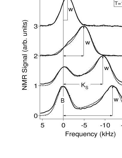
FIG. 1.: Solid lines: ⁷¹Ga OPNMR spectra of sample 10W at $\nu$=$\frac{1}{3}$, taken at $\theta\,$=$\,36.8^{\circ}$ in $B_{\text{tot}}\,$=$\,12\,$T ($f_{\text{o}}$=155.93 MHz). The dashed lines are fits, described in the text.

Fig. 1 shows OPNMR spectra (solid lines) over a range of temperatures at $\nu$=$\frac{1}{3}$. Nuclei within the quantum wells are coupled to the spins of the 2DES via the isotropic Fermi contact interaction[15]. The corresponding well resonance (labeled “W”) is shifted and broadened relative to the signal from the barriers (“B”)[6, 7]. We define $K_{S}$ to be the peak-to-peak splitting between “W” and “B”. The spectra at $\nu$=$\frac{1}{3}$ are well described by a simple two-parameter fit[16] (Fig. 1, dashed lines):

$$I(f)=I_{\text{B}}+I_{\text{W}}=a_{\text{B}}\,g(f)+\!\int^{{}^{K_{S\text{int}}}}_{{}_{0}}\!\!\!\!\!\!\!\!\!\!\!\!\!\!df^{\prime}g(\,f\!-\!f^{\prime}\,)\sqrt{\frac{\textstyle f^{\prime}}{\textstyle K_{S\text{int}}-f^{\prime}}}_{\textstyle,}$$

where $g(f)$ is a 3.5 kHz FWHM Gaussian due to the nuclear spin-spin coupling[15]. The amplitude of the barrier signal, $a_{\text{B}}$, which depends on the OPNMR parameters, was suppressed for small $K_{S}$ spectra. The other parameter of the fit, the intrinsic hyperfine shift of nuclei in the center of each quantum well is $K_{S\text{int}}\,$=$\,A_{c}\>{\cal P}\>n/w$, where $w$ is the width of the well and $A_{c}$ is the hyperfine constant. $K_{S\text{int}}$ can be derived from $K_{S}$ (both in kHz) using the empirical relation $K_{S\text{int}}$=$K_{S}$$+$$1.1$$\times$$(1$$-$$\exp(-K_{S}/2.0))$. A comparison of $K_{S\text{int}}(T$$\rightarrow\,$0) in three different samples yields $A_{c}\,$=$\,(4.5\pm 0.2)\,$$\times\,$$10^{-13}\,$cm³/s, which makes $K_{S\text{int}}$ an absolute measure of the electron spin polarization. An implicit assumption in this model is that the well lineshape is “motionally narrowed”[15]. This requires that the reversed spins (e.g. thermally excited spin waves) are delocalized, so that $\langle S_{z}(\nu,T)\rangle$, averaged over the NMR time scale ($\sim\,$40$\,\mu$sec), appears spatially homogeneous.

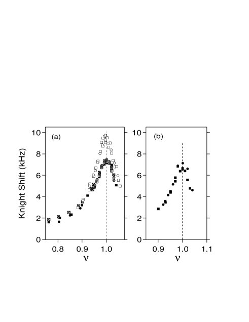
FIG. 2.: $K_{S}(\nu)$ near $\nu$=1 at $T$=1.5 K. (a) Samples 40W (filled symbols, three separate runs) and 10W (open symbols) at $B_{\text{tot}}$=3.6263 T. (b) 40W at $B_{\text{tot}}$=3.2589 T. The densities are $n_{\text{40W}}\,$=$\,6.69\,$$\times\,$$10^{10}\,\text{cm}^{-2}$ and $n_{\text{10W}}\,$=$\,7.75\,$$\times\,$$10^{10}\,\text{cm}^{-2}$.

Using the rotator assembly, we could vary the angle $\theta$ $(-60^{\circ}$$<$$\theta$$<$$60^{\circ})$ between the sample’s growth axis and the applied field $B_{\text{tot}}$, thus changing the filling factor $\nu$=$nhc/eB_{\bot}$ in situ (here $B_{\bot}$$\equiv$$B_{\text{tot}}\!\cos\theta$). Fig. 2 shows $K_{S}$ measurements in the two samples near $\nu$=1. The excellent agreement between positive $\theta$ (squares) and negative $\theta$ (circles) data is consistent with the rotator accuracy of $\pm$$0.1^{\circ}$. We infer the densities $n$ from these measurements assuming that $K_{S}(\theta)$ peaks at $\nu$=1, hence determining $n_{\text{40W}}\,$=$\,6.69\,$$\times\,$$10^{10}\,\text{cm}^{-2}$ and $n_{\text{10W}}\,$=$\,7.75\,$$\times\,$$10^{10}\,\text{cm}^{-2}$, consistent with low-field magnetotransport characterization of the wafers. These values are very robust, as the four independent runs shown in Fig. 2 for sample 40W reproduce $n$ to within $\pm$0.5%.

Note that the sharp peak in $K_{S}$ at $\nu$=1 is quite similar to the “skyrmion feature” previously observed in a higher density sample at stronger $B_{\text{tot}}$ [6]. The “size” of the skyrmion inferred from Fig. 2 ($\tilde{\cal S}$=$\tilde{\cal A}$=3.1 for $B_{\text{tot}}\,$$\sim\,$$3.5\,$T) is slightly larger than before ($\tilde{\cal S}$=$\tilde{\cal A}$=2.6 for $B_{\text{tot}}\,$$\sim\,$$7\,$T)[17], in qualitative agreement with the change in $E_{Z}/E_{C}$[4, 5]. However, a quantitative comparison to the skyrmion model will require data below 1.5 Kelvin, since $\cal P$($\nu$=1) is only $\sim\,$80$\%$ in Fig. 2.

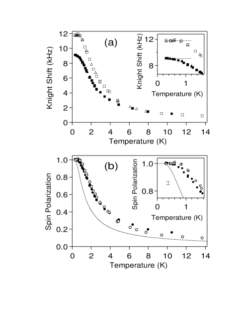
FIG. 3.: Temperature dependence of (a) $K_{S}$ and (b) $\cal P$ for samples 10W (open symbols) and 40W (filled symbols) at $\nu$=$\frac{1}{3}$ (with $B_{\text{tot}}\,$=$\,12\,$Tesla, $\theta_{40\text{W}}$=46.4^∘, and $\theta_{10\text{W}}$=36.8^∘). Dashed line is ${\cal P}^{\ast}(T)$, defined in the text. Insets show the saturation region (note the error bar).

Using the electron densities calculated above, we tilt each sample by the angle $\theta$ necessary to achieve $\nu$=$\frac{1}{3}$ in $B_{\text{tot}}\,$=$\,12\,$Tesla (where $\theta_{40\text{W}}$=46.4^∘, $\theta_{10\text{W}}$=36.8^∘). Fig. 3(a) shows $K_{S}$ as a function of temperature at $\nu$=$\frac{1}{3}$. Two different symbols are used for the 40W data, corresponding to independent cool-downs from room temperature, which demonstrates the reproducibility of the data. The inset shows that $K_{S}$ saturates for both samples at low temperatures, as previously seen at $\nu$=1[6]. In Fig. 3(b) we plot the corresponding temperature dependence of the electron spin polarization, using ${\cal P}(\nu$=$\frac{1}{3},T)\,$=$\,\frac{K_{S\text{int}}(T)}{K_{S\text{int}}(T\!\rightarrow 0)}$. The resulting curves are almost identical for the two samples. The subtle differences that remain might be due to a slightly higher spin stiffness[18] for sample 10W.

The ${\cal P}(\nu$=$\frac{1}{3},T)$ data in Fig. 3(b) probe the neutral spin-flip excitations of a fractional quantum Hall ferromagnet. For comparison, the dashed line is the polarization ${\cal P}^{\ast}(T)$ calculated for non-interacting electrons at $\nu$=1, where ${\cal P}^{\ast}(T)$=$\tanh(E_{Z}/4k_{B}T)$, $B_{\text{tot}}$=12 T, and $g^{\ast}$= $-$0.44. Both ${\cal P}(\nu$=$1,T)$[6, 19] and ${\cal P}(\nu$=$\frac{1}{3},T)$ saturate at higher temperatures than ${\cal P}^{\ast}(T)$, however, the data at $\nu$=$\frac{1}{3}$ lie much closer to this ${\cal P}^{\ast}(T)$ limit. Fitting $\tanh(\Delta/4k_{B}T)$ to the saturation region of the data, we find $\Delta\,$$\approx\,$$2E_{Z}$ at $\nu$=$\frac{1}{3}$, as opposed to $\Delta\,$$\approx\,$$10E_{Z}$ at $\nu$=1[6]. We also note that the 40W data set is very well described by $\Delta\,$$=\,$$1.82\,E_{Z}$ over the entire temperature range, in sharp contrast to the behavior at $\nu$=1. These results are consistent with the spin stiffness being much less at $\nu$=$\frac{1}{3}$ than at $\nu$=1[18]. While a recent numerical result[20] is in qualitative agreement with the data in Fig. 3(b), it remains to be seen whether other theoretical approaches, such as those used at $\nu$=1[21], can be modified to explain these data.

FIG. 4.: Dependence of $K_{S}$ on filling factor at fixed temperature. Open circles: sample 10W at $T$=0.77 K, filled circles: sample 40W at $T$=0.46 K; open and filled diamonds: 10W and 40W at $T$=1.5 K, respectively. Solid and dashed lines are described in the text.

The Knight shift was also measured at fixed temperature as a function of sample tilt angle, with $B_{\text{tot}}$=12 T. Fig. 4(a) shows $K_{S}(\nu)$ near $\nu$=$\frac{1}{3}$ for sample 10W at $T$=0.77 K, and for sample 40W at $T$=0.46 K. By these low temperatures, $K_{S}(\nu$=$\frac{1}{3})$ has essentially saturated for both samples. The data in Fig. 4(a) show that $K_{S}(\nu)$ drops on either side of $\nu$=$\frac{1}{3}$, a result that is reminiscent of earlier measurements near $\nu$=1[6]. The $K_{S}(\nu$$\sim$$\frac{1}{3})$ feature is distinctly “sharper” for sample 10W as opposed to sample 40W. This difference between the samples is not an artifact of the temperatures plotted, as Fig. 4(b) shows that the distinction is already present by $T$=1.5 K. In order to measure $K_{S}(\nu)$ this accurately, we took into account the extrinsic tilt-angle dependence of the barrier frequency (Fig. 4(b), solid and dashed curves) caused by a paramagnetic rotation stage.

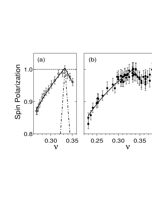
FIG. 5.: Dependence of $\cal P$ on filling factor at fixed temperature. (a) 10W at $T$=0.77 K (open circles); Eq. (1) with $\nu_{o}$=$\frac{1}{3}$ for: $\tilde{\cal A}$=$\tilde{\cal S}$=0 (dashed line), $\tilde{\cal A}$=0.085 and $\tilde{\cal S}$=0.15 (solid line), and $\tilde{\cal A}$=$\tilde{\cal S}$=1 (dash-dotted line). (b) 40W at $T$=0.46 K (filled circles); Eq. (1) with $\nu_{o}$=$\frac{1}{3}$, $\tilde{\cal A}$=0.053 and $\tilde{\cal S}$=0.10 (solid line).

The $K_{S}(\nu)$ data shown in Fig. 4(a) are converted to the corresponding electron spin polarization ${\cal P}(\nu)$ $\equiv\frac{K_{S\text{int}}(\nu)}{K_{S\text{int}}(\nu=1\!/3)}$, and are plotted in Fig. 5. The polarization of both samples decreases as $\nu$ is varied away from $\frac{1}{3}$, despite the presence of the 12 T field! Perhaps even more remarkably, ${\cal P}(\nu)$ decreases monotonically as $\nu$ is lowered below $\frac{1}{3}$ over the observed range ($\frac{\delta\nu}{1/3}\sim-30\%$). This strongly suggests that the charged quasiparticles and quasiholes of the $\nu$=$\frac{1}{3}$ ground state involve electron spin flips.

$\nu\>$$\downarrow$ $\backslash$ T$\>\rightarrow$	1.5 K	0.9 K	0.7 K	0.5 K	0.3 K
1/3	0 $\%$	4 $\%$	4 $\%$	3 $\%$	5 $\%$
0.29	2 $\%$	12 $\%$	20 $\%$	36 $\%$	32 $\%$
0.27	12 $\%$	21 $\%$	45 $\%$	69 $\%$	53 $\%$

TABLE I.: The percentage increase of the well linewidth for sample 10W, relative to the value of 5.2 kHz at $T$=1.5 K and $\nu$=$\frac{1}{3}$.

A second, independent measurement provides further evidence for the presence of reversed spins below $\nu$=$\frac{1}{3}$. While the high temperature spectra are “motionally narrowed”[15], Table I shows that the well lineshape broadens dramatically at low temperatures below $\nu$=$\frac{1}{3}$. This change in the lineshape indicates that the time-averaged $\langle S_{z}\rangle$ is no longer spatially homogeneous. The inhomogeneity requires the existence of spin-reversed regions, that become localized over the NMR time scale as the temperature is lowered below $\sim$0.5 K ($\sim$0.3 K) for sample 10W (40W)[16]. In order to avoid the complication of a spatially inhomogeneous $\langle S_{z}\rangle$, the data presented in Fig. 5 were taken at temperatures that were just low enough to saturate $K_{S}(T)$ at $\nu$=$\frac{1}{3}$.

To quantify the rate of depolarization in Fig. 5, we extend a simple model previously used near $\nu$=1[6]. Our model parametrizes the effect of interactions in the neighborhood of a ferromagnetic filling factor $\nu_{o}$$<$1. We assume that adding a quasiparticle (or quasihole) to the ground state causes $\tilde{\cal S}$ (or $\tilde{\cal A}$) electron spins to flip[17]. Within this model, the electron spin polarization is:

$${\cal P}(\nu)=1+2\Bigl{(}\frac{1}{\nu}-\frac{1}{\nu_{o}}\Bigr{)}\Bigl{(}\tilde{\cal S}\,\Theta(\nu\!-\!\nu_{o})-\tilde{\cal A}\,\Theta(\nu_{o}\!-\!\nu)\Bigr{)},$$ (1)

where $\Theta(x)\equiv\{\,1,\,x\!\geq\!0;\>\text{and}\>\>0,\,x\!<\!0\,\}$. Using Eq. (1) to fit the data near $\nu_{o}$=$\frac{1}{3}$ (solid lines), we find:

$\begin{array}[]{lll}10\text{W:}&\tilde{\cal A}=0.085\pm 0.005,&\tilde{\cal S}=0.15\pm 0.04\\ 40\text{W:}&\tilde{\cal A}=0.053\pm 0.008,&\tilde{\cal S}=0.10\pm 0.03.\\ \end{array}$

For comparison, the earliest theory[1, 11] of the $\nu$=$\frac{1}{3}$ ground state assumed spin-polarized quasiparticles and quasiholes, i.e., $\tilde{\cal S}$=$\tilde{\cal A}$=0 (Fig. 5, dashed line). Subsequent calculations [10] considered the possibility of spin-reversed quasiparticles and quasiholes, i.e., $\tilde{\cal S}$=$\tilde{\cal A}$=1 (Fig. 5, dash-dotted line). However, both the early calculations and the more recent studies of skyrmion excitations near $\nu$=$\frac{1}{3}$[22, 23] suggest $\tilde{\cal S}$=$\tilde{\cal A}$=0 for strong magnetic fields. On the other hand, our small, non-zero values are within the bounds set by transport measurements at ambient[24] and high[25] pressures.

A much more difficult feature to understand is the fact that our measured values are fractional ($\tilde{\cal S}\,$$\sim\,$$\tilde{\cal A}\,$$\sim\,$0.1), since the magnetic field should make $\langle S_{z}\rangle$ a good quantum number for the N particle system[10]. Of course, our experiment does not have the resolution to see the effect of adding a single quasiparticle to the $\nu$=$\frac{1}{3}$ ground state, thus these values for $\tilde{\cal S}\,$ and $\tilde{\cal A}\,$ are the average numbers of flipped spins per quasiparticle and quasihole. Nevertheless, Eq. (1), which assumes that all quasiholes (or quasiparticles) behave in exactly the same way, does a remarkably good job fitting our data over the range (0.23$<$$\nu$$<$0.36). This model is expected to break down outside the “dilute” quasiparticle limit (i.e., when $\nu$ gets “too far” from $\frac{1}{3}$), since $\tilde{\cal S}$ and $\tilde{\cal A}$ are independent of $\nu$. Surprisingly, the above fit actually passes through $\nu$=$\frac{2}{7}$ without modification. High field magnetotransport measurements on samples taken from the same wafer as 10W show much more structure, with well-developed minima in $\rho_{xx}$ at $\nu$=$\frac{1}{3},\frac{2}{5},\frac{2}{7},$ and $\frac{1}{5}$ at $T\,$=$\,300$ mK[14, 26].

The possible explanations of these values ($\tilde{\cal S}\,$$\sim\,$$\tilde{\cal A}\,$$\sim\,$0.1) are constrained by many different aspects of the data. For example, the values of $\tilde{\cal S}$ and $\tilde{\cal A}$ do not appear to change up to $T$=1.5 K. Furthermore, the motional narrowing of the NMR line requires that the time-averaged electron spin polarization is spatially uniform for all $\nu$.

We thank S. M. Girvin, A. H. MacDonald, N. Read, and S. Sachdev for helpful discussions. We also thank K. E. Gibble, R. L. Willett, and K. W. Zilm for experimental assistance. This work was supported by NSF CAREER Grant $\#$DMR-9501925.

REFERENCES

- [1] R. B. Laughlin, Phys. Rev. Lett. 50, 1395 (1983).
- [2] D. C. Tsui, H. L. Stormer, and A. C. Gossard, Phys. Rev. Lett. 48, 1559 (1982).
- [3] B. I. Halperin, Helv. Phys. Acta 56, 75 (1983).
- [4] S. L. Sondhi, A. Karlhede, S. A. Kivelson, and E. H. Rezayi, Phys. Rev. B 47, 16419 (1993).
- [5] H. A. Fertig, L. Brey, R. Côté, and A. H. MacDonald, Phys. Rev. B 50, 11018 (1994).
- [6] S. E. Barrett et al., Phys. Rev. Lett. 74, 5112 (1995).
- [7] R. Tycko et al., Science 268, 1460 (1995).
- [8] A. Schmeller, J. P. Eisenstein, L. N. Pfeiffer, and K. W. West, Phys. Rev. Lett. 75, 4290 (1995).
- [9] E. H. Aifer, B. B. Goldberg, and D. A. Broido, Phys. Rev. Lett. 76, 680 (1996).
- [10] T. Chakraborty and P. Pietiläinen, The Quantum Hall Effects: Integral and Fractional, 2 ed.(Springer, Berlin, 1990).
- [11] The Quantum Hall Effect, 2 ed., edited by R. E. Prange and S. M. Girvin, (Springer, New York, 1990).
- [12] Perspectives in Quantum Hall Effects, edited by S. Das Sarma and A. Pinczuk, (Wiley, New York, 1997).
- [13] S. E. Barrett, R. Tycko, L. N. Pfeiffer, and K. W. West, Phys. Rev. Lett. 72, 1368 (1994).
- [14] L. N. Pfeiffer et al., Appl. Phys. Lett. 61, 1211 (1992).
- [15] C. P. Slichter, Principles of Magnetic Resonance (Springer, New York, 1990), 3rd ed.
- [16] N. N. Kuzma et al., Science (July 31,1998).
- [17] Throughout this Letter, we use the convention that ==0 in the non-interacting limit, instead of the original definition [6], ==1, in the same limit.
- [18] K. Moon et al., Phys. Rev. B 51, 5138 (1995).
- [19] M. J. Manfra et al., Phys. Rev. B 54, R 17 327 (1996).
- [20] T. Chakraborty and P. Pietiläinen, Phys. Rev. Lett. 76, 4018 (1996).
- [21] N. Read and S. Sachdev, Phys. Rev. Lett. 75, 3509 (1995); M. Kasner and A. H. MacDonald, ibid. 76, 3204 (1996); R. Haussmann, Phys. Rev. B 56, 9684 (1997); C. Timm, P. Henelius, A. W. Sandvik, and S. M. Girvin, Phys. Rev. B 58, 1464 (1998).
- [22] R. K. Kamilla, X. G. Wu, and J. K. Jain, Solid State Commun. 99, 289 (1996).
- [23] K. H. Ahn and K. J. Chang, Phys. Rev. B 55, 6735 (1997).
- [24] R. J. Haug et al., Phys. Rev. B 36, 4528 (1987).
- [25] D. R. Leadley et al., Phys. Rev. Lett. 79, 4246 (1997).
- [26] R. L. Willett (private communication).