Distributions of the Conductance
and its Parametric Derivatives in Quantum Dots

Abstract

Full distributions of conductance through quantum dots with single-mode leads are reported for both broken and unbroken time-reversal symmetry. Distributions are nongaussian and agree well with random matrix theory calculations that account for a finite dephasing time, $\tau_{\varphi}$, once broadening due to finite temperature $T$ is also included. Full distributions of the derivatives of conductance with respect to gate voltage $P(dg/dV_{g})$ are also investigated.

The remarkable success of random matrix theory (RMT) and other noninteracting theories in describing the statistics of quantum transport in mesoscopic electronic systems is surprising considering that electron-electron interactions not accounted for in the theory are sizable compared to other energy scales in these systems. In the last few years, an essentially complete statistical theory of mesoscopic fluctuation and interference effects in disordered or chaotic (irregularly shaped) quantum dots and wires has been formulated using these methods [1, 2, 3] and has recently been extended beyond the “universal” regime to include short-trajectory effects [4], clarifying the degree to which these theories are indeed universal [5].

But how seriously should a noninteracting theory be taken when describing real metallic or semiconductor structures? Apparently, this depends on the quantity being measured. For instance, the mean and variance of mesoscopic conductance fluctuations in open quantum dots and disordered wires appear to be in good agreement with random matrix theory [1] and sigma model calculations [6] once temperature and dephasing effects are included, whereas the distribution of energies needed to add subsequent electrons to a closed dot does not appear distributed according to the famous Wigner-Dyson law, a basic result of RMT[7].

In this Letter we carry out a stringent test of statistical theories of mesoscopic conductance fluctuations by measuring the full distribution $P(g)$ of conductance, $g$, through chaotically shaped ballistic quantum dots. Conductance distributions of quantum dots have previously been calculated within RMT [8, 9], including the effects of dephasing [1, 10, 11, 12]. The distributions are universal for any fully chaotic or disordered dot, sensitive only to whether time reversal symmetry is obeyed ($\beta=1$) or broken ($\beta=2$), controlled by adding a magnetic field, $B>\,\sim\phi_{o}/A_{dot}$, where $A_{dot}$ is the dot area and $\phi_{o}=h/e$ is the flux quantum. RMT yields quite interesting (i.e. strongly nongaussian) distributions when one or two quantum modes connect the dot to bulk reservoirs. To date, however, experimental measurements of these nongaussian distributions have not been reported, first because it is difficult to generate large ensembles of statistically identical devices, and second because dephasing, which acts roughly as extra modes coupling the dot to the environment, leads to nearly gaussian distributions [12, 13, 14]. To see the nongaussian distributions, dephasing rates and temperatures comparable to the quantum level spacing are required. We solve the first problem, of obtaining large ensembles, by using electrostatic shape distortion of gate-defined quantum dots in a GaAs/AlGaAs heterostructure [13].

We find good agreement between the experimental distributions and the RMT predictions over a broad range of temperatures once thermal averaging is properly accounted for. The agreement is particularly surprising since we are investigating the case of single-mode leads, $N=1$. This is the transition between open and closed dots; for any lower conductance to the dot, electron-electron interactions in the form of Coulomb blockade dominate transport, leading to dramatic departures from a noninterating picture [15]. Here $N$ denotes the number of modes or channels in both the left and right leads, giving dimensionless lead conductances $g_{\rm l}=g_{\rm r}=2N$, where $g$ is in units of $e^{2}/h$.

Distributions of mesoscopic conductance at $T=0$ may be calculated within RMT for any number of modes $N$ in the leads using the Landauer formula, $g=2\;Tr(tt^{\dagger})$, by assuming that the $2N\times 2N$ scattering matrix $S=\left({\matrix{r&t^{\prime}\cr t&r^{\prime}\cr}}\right)$ is a random unitary matrix reflecting the ergodicity of chaotic scattering [1]. For single-mode leads, $N=1$, this calculation gives $P(g)={1\over 2}(g/2)^{-1+\beta/2}$ [8, 9], shown as dashed lines in Fig. 1. Notice that the $\beta=1$ distribution is skewed toward smaller conductance, with average conductance $\langle g\rangle_{\beta=1}=2/3$, while the $\beta=2$ distribution is constant between $0$ and $2$ with $\langle g\rangle_{\beta=2}=1$. The lower average conductance for $\beta=1$ results from coherent backscattering, analogous to weak localization, at $B=0$.

Dephasing, or the loss of quantum coherence, can be modeled within RMT by expanding the scattering matrix $S$ to include a fictitious voltage lead that supports a number of modes $\gamma_{\varphi}=2\pi\hbar/(\tau_{\varphi}\Delta)$, where $\Delta={2\pi\hbar^{2}}/{m^{*}A_{dot}}$ is the spin-degenerate mean level spacing and $\tau_{\varphi}$ is the characteristic dephasing time [10, 11]. A recent improvement to the voltage-probe model that accounts for the spatially distributed nature of the dephasing process considers the limit of a voltage lead supporting an infinite number of modes, each with vanishing transmission, allowing a continuous value for the dimensionless dephasing rate $\gamma_{\varphi}$ [12]. As described below, the general effect of dephasing is to make $P(g)$ narrower and roughly gaussian, and to reduce the difference in mean conductance upon breaking time reversal symmetry, $\delta g=\langle g\rangle_{\beta=2}-\langle g\rangle_{\beta=1}$.

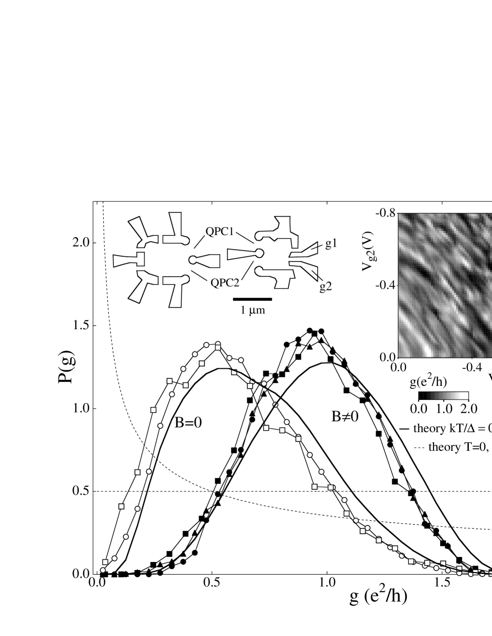
FIG. 1.: Conductance distributions for $B=0$ (open circles), 40 mT (filled circles) and 60 mT (filled triangles) for the $0.5\;\mu{\rm m}^{2}$ device at 100 mK, and for $B=0$ (open squares) and 25 mT (filled squares) for the $1.0\;\mu{\rm m}^{2}$ device at 45 mK, along with the theoretical distributions for $kT/\Delta=0.61$, $\gamma_{\varphi}=0.3$ (solid curves) and $T=0$, $\gamma_{\varphi}=0$ (dashed curves). Upper left inset: Pattern of gates defining each quantum dot. Upper right inset: Conductance through $0.5\;\mu{\rm m}^{2}$ dot as a function of the two shape-distorting gates $V_{g1}$ and $V_{g2}$.

Measurements on two lateral quantum dot with areas $0.5\;\mu{\rm m}^{2}$ ($\Delta=\rm 14\;meV$) and $1.0\;\mu{\rm m}^{2}$ ($\Delta=\rm 7.1\;meV$) are reported. The devices (see Fig. 1 inset) are defined using Cr/Au depletion gates 90 nm above a two-dimensional electron gas (2DEG) formed at a GaAs/Al_0.3Ga_0.7As heterointerface. Multiple gates are used to allow independent control of the two point-contact leads as well as dot shape. Sheet density $n=2\times 10^{11}\;\rm cm^{-2}$ and mobility $\rm\mu=1.4\times 10^{5}\;{cm^{2}}/{Vs}$ give an elastic mean free path of $\sim 1.5\;\mu$m, larger than all device dimensions, so that transport within the dots is ballistic. The dots were measured in a dilution refrigerator over a range of electron temperatures from 45 mK to 750 mK using standard 4-wire lock-in techniques at 43 Hz (13 Hz) and less than 7 $\mu$V (2 $\mu$V) bias voltage for the $0.5\;\mu{\rm m}^{2}$ ($1.0\,\mu{\rm m}^{2}$) device. Electron temperature was determined from a fit to the average Coulomb blockade peak width, as described in [16].

Experimental conductance distributions $P(g)$ for $|B|\ll\phi_{o}/A_{dot}$ ($\beta=1$) and $|B|\gg\phi_{o}/A_{dot}$ ($\beta=2$) are shown in Fig. 1. Each histogram contains $\sim 1000$ independent samples measured at fixed $B$ drawn from the random landscape of conductance fluctuations in the space of $V_{g1}$ and $V_{g2}$ (inset Fig. 1). Note that the conductance landscape appears random and the average roughly constant over the shape-distortion landscape. The asymmetry of the $\beta=1$ distribution is striking, in contrast with previous measurements [13, 18] which found roughly gaussian distributions due to thermal averaging and dephasing. The average conductance at $\beta=2$ is $\sim e^{2}/h$ as expected from RMT, with a small (4%) deviation at the lowest temperatures possibly due to imperfect quantum point contacts enchanced by incipient charging effects [19, 20]. Once time-reveral symmetry is broken, the distribution becomes insensitive to magnetic field for the relatively small fields used in the experiment (the cyclotron radius is always larger than the dot size). For instance, though $g(B)$ are uncorrelated at $B=40$ mT and 60 mT, $P(g)$ at these magnetic field values are nearly identical ($\phi_{o}/A_{dot}$ is $\sim 8$ mT for the $0.5\;\mu\rm m^{2}$ device).

Before the experimental distributions can be compared to theory it is necessary to measure the dephasing rate, since $P(g)$ depends on $\gamma_{\varphi}$. Values for $\gamma_{\varphi}$ are measured from the weak localization correction to the average conductivity, $\delta g=\langle g\rangle_{\beta=2}-\langle g\rangle_{\beta=1}$ using the results of Ref. [12], as shown in Fig. 2(b). The values for $\gamma_{\varphi}(T)$ agree with previous measurements found using a variety of magnetotransport methods including weak localization and the power spectrum of conductance fluctuations [21], and extend those measurements to lower temperatures. Unfortunately, while $\langle g\rangle$ depends on temperature only through $\gamma_{\varphi}$ (which is why weak localization is particularly useful for measuring dephasing), the full distributions $P(g)$ depend on temperature both implicitly through dephasing and explicitly through thermal averaging. The combined effects of dephasing and thermal smearing must in general be evaluated numerically, which we do as follows. A set of values $y=\sum\nolimits_{i}{w_{i}(T)x_{i}}$ is generated by summing independent samples $x_{i}$ drawn from the known distribution $P(x,\gamma_{\varphi})$ [12], weighted by the derivative of the Fermi function, $w_{i}=\tilde{\Delta}f^{\prime}([i+\delta]\tilde{\Delta})$, where $f^{\prime}(\epsilon)={d\over d\epsilon}(1+e^{\epsilon/kT})^{-1}$, $\delta$ is a binning offset, and $\tilde{\Delta}$ is the level broadening, itself dependent on $\gamma_{\varphi}$ as described below. By sampling over ensembles of $x$ values, a distribution $P(y)$ is obtained (the result is insensitive to the choice of $\delta$ for sufficiently large $T$). Note that neither fluctuations in level spacing nor fluctuations in the coupling between the levels and modes in the leads are included in this simple model.

Both dephasing and temperature averaging tend to make $P(g)$ roughly gaussian, in which case $P(g)$ can be characterized by its mean and variance. As discussed above, the mean, $\langle g\rangle$, is not affected by thermal averaging. The variance is reduced both by dephasing, well approximated by the interpolation formula ${\rm Var}\,x=(a+b\gamma_{\varphi})^{-2}$ where $a=\sqrt{3}\;(\sqrt{45/16})$ and $b=1\;(\sqrt{1/3})$ for $\beta=2\;(1)$ [10], and by thermal averaging, ${\rm Var}\,y=\sum\nolimits_{i}w_{i}^{2}\>{\rm Var}\,x$. At temperatures exceeding the level broadening this sum can be well approximated by an integral,

$${\rm Var}\,y=\tilde{\Delta}\Bigl{[}\int_{-\infty}^{\infty}[f^{\prime}(\epsilon)]^{2}d\epsilon\Bigr{]}\,{\rm Var}\,x={\tilde{\Delta}\over{6kT}}\,{\rm Var}\,x.$$ (1)

The integral form differs from the sum by less than 1% for $kT\geq 0.6\tilde{\Delta}$. For the devices studied in this paper, this condition is easily satisfied, and Eq. (1) is applicable at all measured temperatures.

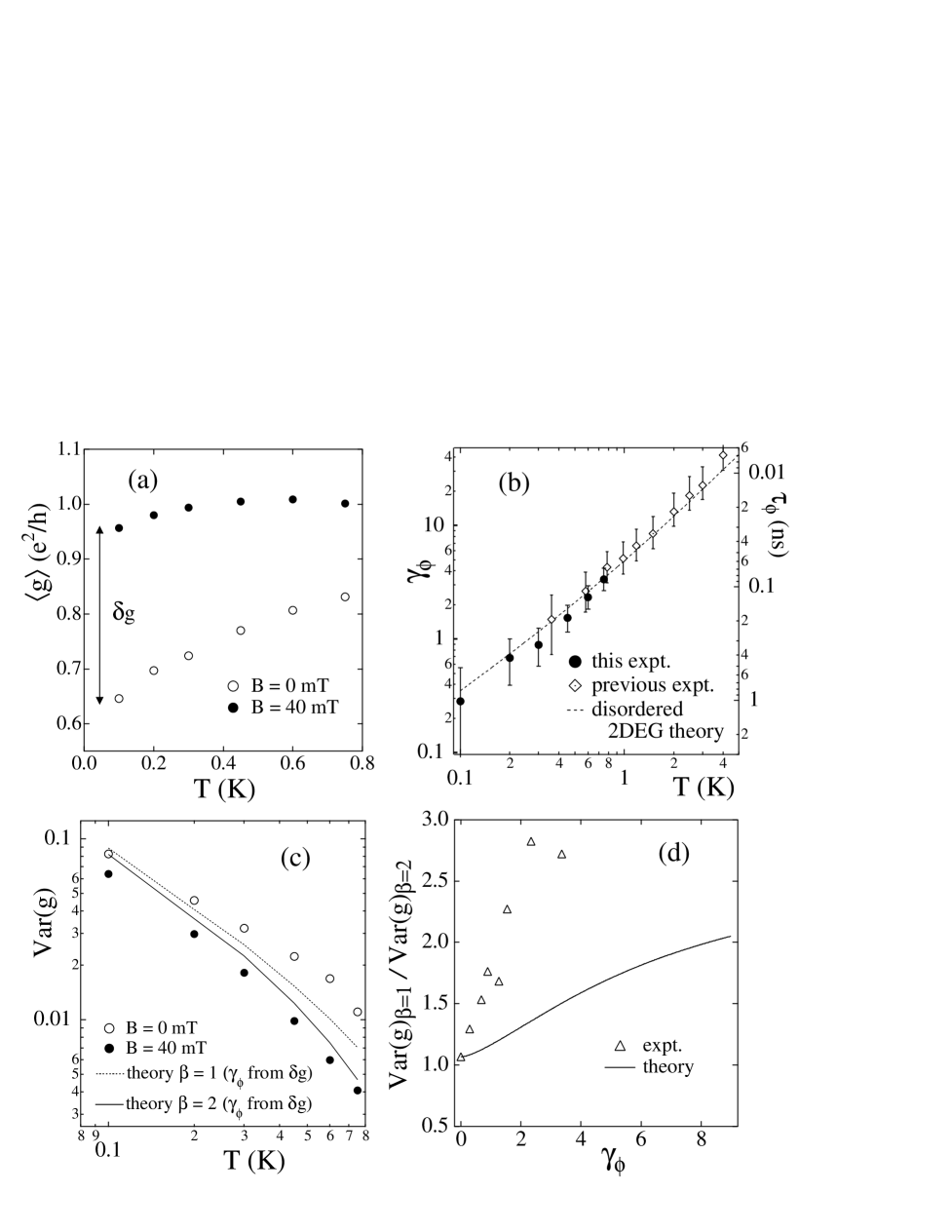
FIG. 2.: (a) Average conductance $\langle g\rangle$ as a function of temperature $T$ for $B=0$ and 40 mT for the 0.5 $\mu\rm m^{2}$ dot. (b) Normalized dephasing rate $\gamma_{\varphi}$ and dephasing time $\tau_{\varphi}$ determined from $\delta g(T)$ for the 0.5 $\mu\rm m^{2}$ dot. Note agreement with previously measured $\gamma_{\varphi}(T)$ in a 0.4 $\mu\rm m^{2}$ dot [21]. (c) Variance of conductance for $B=0$ and $B=40$ mT, corresponding to expected variance for $\beta=1$ (dashed) and $\beta=2$ (solid) including thermal smearing and dephasing effects (see text). (d) Variance ratio ${\rm Var}\>g_{\beta=1}/{\rm Var}\>g_{\beta=2}$ as a function of dephasing rate $\gamma_{\varphi}$.

The thermal averaging procedure given above takes energy intervals of size $\tilde{\Delta}$ to be statistically independent. Dephasing contributes to level broadening by an amount proportional to the dephasing rate, which can be taken into account by defining the level broadening to be

$${\tilde{\Delta}=\Delta\left(1+\gamma_{\varphi}/2\right)}.$$ (2)

Inserting this definition into Eq. (1) reproduces a number of previously obtained results for Var $g$ in various limits: ($\gamma_{\varphi}\ll 1$, $T\ll\Delta$) [8, 9] ; ($\gamma_{\varphi}\ll 1$, $T\gg\Delta$)[6]; ($\gamma_{\varphi}\gg 1$, $T\ll\Delta$) [10, 11]; and ($\gamma_{\varphi}\gg 1$, $T\gg\Delta$) [6]. The measured variances of the conductance distributions for $\beta=1$ and $\beta=2$ as a function of temperature are compared to our thermal averaging model in Fig. 2(c). The two are in good overall agreement, however, the ratio of variances, ${\rm Var}\>g_{\beta=1}/{\rm Var}\>g_{\beta=2}$ shows significant disagreement between experiment and theory which remains unexplained. In particular, the experimental ratio of variances is considerably larger than predicted, as seen in Fig. 2(d). This ratio is an interesting quantity because, like $\delta g$, it does not suffer thermal averaging within the simple model considered here. Despite the disagreement in the ratio of variances, the RMT results for $P(g)$ are generally in very good agreement with experiment across a broad range of temperatures, as seen in Fig. 3.

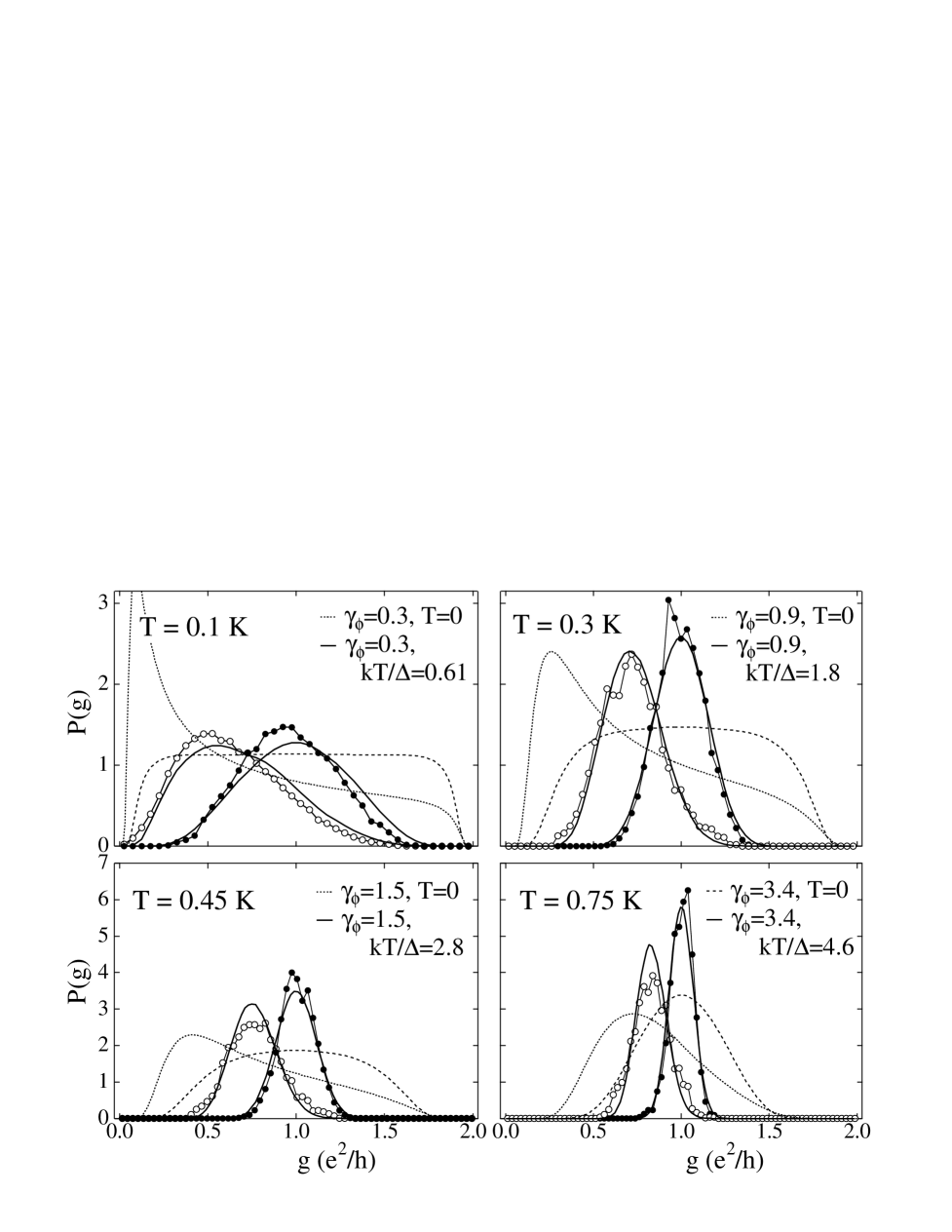
FIG. 3.: Measured conductance distributions for $B=0$ (open circles) and 40 mT (closed circles) for the $0.5\,\mu\rm m^{2}$ dot at four temperatures. Curves show theoretical $\beta=1$ (dotted) and $\beta=2$ (dashed) distributions for $T=0$ and for measurement temperatures (solid). $T=0$ distributions are determined using the method of Ref. [12]. Thermal distributions are calculated according to the sampling procedure described in the text.

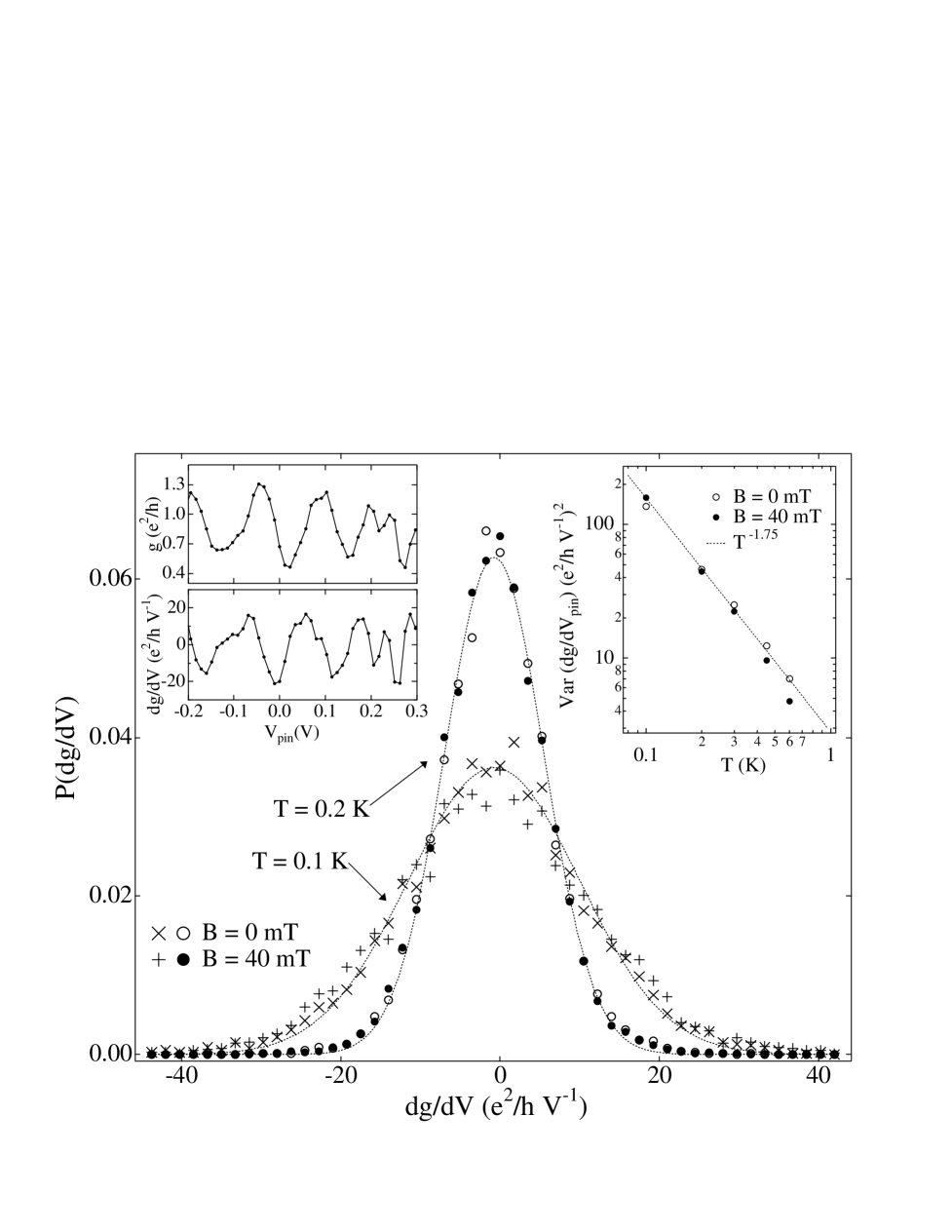
FIG. 4.: Conductance derivatives $P(dg/dV_{g})$ at $B=0$ and 40 mT for $T=0.1$ K and $T=0.2$ K. Upper right inset shows Var($dg/dV_{g}$) as a function of temperature, which exhibits a $T^{-1.75}$ dependence. Upper left inset shows fluctuating conductance $g$ and derivative $P(dg/dV_{g})$ as function of gate voltage.

We have also investigated distributions of parametric derivatives of conductance with respect to magnetic field $dg/dB$ and gate voltage, $dg/dV_{g}$. These quantities are of considerable interest as they are the open-system analogs of the well-studied “level velocities” $dE/dX$ of the energy levels in closed quantum chaotic systems [5]. Distributions of parametric derivatives of conductance have recently been investigated theoretically using an RPA “charged fluid” model, which gave interesting nongaussian distributions for both $\beta=1$ and $\beta=2$ [22]. We have investigated both $P(dg/dB)$ and $P(dg/dV_{g})$ in single-mode dots, and find both distributions are well described by gaussians due to dephasing and thermal averaging. Here we focus on $P(dg/dV_{g})$, shown in Fig. 4 for zero and nonzero magnetic field, at $T=0.1$ mK and $0.2$ mK. Thermal averaging dominates the width of the distribution. We find ${\rm Var}\,g\propto\,T^{-1.75}$. Distributions of $dg/dB$ are also roughly gaussian, with variances of 9.65 $\rm{mT}^{-2}$ at $T=0.1$ K and 0.939 $\rm{mT}^{-2}$ at $T=0.5$ K. To observe deviations from gaussian distributions of parametric derivatives, lower temperatures than those needed to see nongaussian $P(g)$ are required.

In summary, we have measured distribution of conductance and its derivatives using large ensembles of shape-deformable chaotic GaAs quantum dots with single-mode leads. Accurate control of lead conductances and low temperature allow the nontrivial predictions of RMT to be observed. We find that a thermally averaged RMT provides a good description of the measured distributions, though some features, in particular the ratio of variances ${\rm Var}\>g_{\beta=1}/{\rm Var}\>g_{\beta=2}$, are inconsistent with the present model and remain to be resolved.

We thank I. Aleiner and K. Matveev for useful discussions. We gratefully acknowledge support at Stanford from the Army Research Office under Grant DAAH04-95-1-0331, the Office of Naval Research YIP program under Grant N00014-94-1-0622, the NSF-NYI and PECASE programs, the A. P. Sloan Foundation, and support for AGH from the Fannie and John Hertz Foundation. We also acknowledge support from JSEP under Grant DAAH04-94-G-0058. PWB acknowledges support from the NSF under grants DMR 94-16910, DMR 96-30064, and DMR 94-17047.

REFERENCES

- [1] C. W. J. Beenakker, Rev. of Mod. Phys. 69, 731 (1997).
- [2] K. Efetov, Supersymmetry in Disorder and Chaos (Cambridge University Press, Cambridge, 1997).
- [3] For a collection of recent articles, see the special issue of Chaos, Solitons and Fractals, Edited by K. Nakamura, 8 971-1411 (1997).
- [4] A. V. Andreev, O. Agam, B. D. Simons and B. L. Altshuler, Phys. Rev. Lett. 76, 3947 (1996); B. A. Muzykantskii and D. E. Khmelnitskii, JETP Lett. 62, 68 (1995).
- [5] B. L. Altshuler and B. D. Simons, in Mesoscopic Quantum Physics edited by E. Akkermans, G. Montambaux, J.-L. Pichard and J. Zinn-Justin (Elsevier, Amsterdam, 1995).
- [6] K.B. Efetov, Phys. Rev. Lett.74, 2299 (1995).
- [7] U. Sivan et al., Phys. Rev. Lett. 77, p. 1123 (1996); F. Simmel, T. Heinzel and D. A. Wharam, Europhys. Lett. 38, 123 (1997); S. Patel et al., cond-mat/9708090 (1997).
- [8] R. A. Jalabert, J.-L. Pichard and C. W. J. Beenakker, Europhysics Letters 27, 255 (1994).
- [9] H. U. Baranger and P. A. Mello, Phys. Rev. Lett. 73, 142 (1994).
- [10] H. U. Baranger and P. A. Mello, Phys. Rev. B 51, 4703 (1995).
- [11] P. W. Brouwer and C. W. J. Beenakker, Phys. Rev. B 51, 7739 (1995).
- [12] P. W. Brouwer and C. W. J. Beenakker, Phys. Rev. B 55, 4695 (1997).
- [13] I. H. Chan et al., Phys. Rev. Lett. 74, 3876 (1995).
- [14] E. McCann and I. V. Lerner, cond-mat/9712160 (1997).
- [15] L.P. Kouwenhoven et al., in Mesoscopic Electron Transport, NATO ASI Series E, vol. 345, edited by L.L. Sohn, L.P. Kouwenhoven and G. Schön (Kluwer, Dordrecht, 1997).
- [16] J. A. Folk et al., Phys. Rev. Lett. 76, 1699 (1996).
- [17] C. W. J. Beenakker and H. van Houten, in Solid State Physics, Vol. 44, 1.
- [18] Y. Lee, G. Faini, and D. Mailly, Chaos, Solitons & Fractals 8, 1325 (1997).
- [19] A. Furusaki and K. Matveev, Phys. Rev. Lett. 75, p. 709 (1995).
- [20] I. Aleiner and L. Glazman, cond-mat/9710195 (1997).
- [21] A. G. Huibers et al., cond-mat/9708170 (1997).
- [22] P. W. Brouwer et al., Phys. Rev. Lett. 79, 913 (1997).