Observability of counterpropagating modes at fractional-quantum-Hall edges

Abstract

When the bulk filling factor is $\nu=1-1/m$ with $m$ odd, at least one counterpropagating chiral collective mode occurs simultaneously with magnetoplasmons at the edge of fractional-quantum-Hall samples. Initial experimental searches for an additional mode were unsuccessful. In this paper, we address conditions under which its observation should be expected in experiments where the electronic system is excited and probed by capacitive coupling. We derive realistic expressions for the velocity of the slow counterpropagating mode, starting from a microscopic calculation which is simplified by a Landau-Silin-like separation between long-range Hartree and residual interactions. The microscopic calculation determines the stiffness of the edge to long-wavelength neutral excitations, which fixes the slow-mode velocity, and the effective width of the edge region, which influences the magnetoplasmon dispersion.

I Introduction

A two-dimensional (2D) electron system in a strong transverse magnetic field can exhibit the quantum Hall (QH) effect.[2, 3] This effect occurs when the electron fluid becomes incompressible[4] at magnetic-field-dependent densities. The physical origin of the incompressibility, i.e., of an energy gap for the excitation of unbound particle-hole pairs, is quite different for the integer and fractional QH effects. In the integer case, the incompressibility arises from Landau quantization of the kinetic energy of a charged 2D particle in a transverse magnetic field, while in the fractional case it is a consequence of electron-electron interactions. In both cases, however, the only low-lying excitations are localized at the boundary of the QH sample. In a magnetic field, collective modes, known as edge magnetoplasmons[5] (EMP), occur at the edge of a 2D electron system even when the bulk is compressible. Outside of the QH regime, however, these modes have a finite lifetime[5] for decay into incoherent particle-hole excitations and are most aptly described using a hydrodynamic picture. In the QH regime, provided that the edge of the 2D electron system is sufficiently sharp,[6] the microscopic physics simplifies and there is no particle-hole continuum into which the modes can decay. Generalizations of models familiar from the study of one-dimensional (1D) electron systems[7] can then be used to provide a fully microscopic description of integer[8] and fractional[9, 10] QH edges. In these models, EMP appear as free Bose particles in the bosonized description of a chiral 1D electron gas.

In this work, we consider the edge of a 2D electron system in the regime where the fractional QH effect occurs, i.e., for filling factors $\nu<1$ and $\nu$ equal to one of the filling factors at which the bulk of the 2D system is incompressible. The fractional quantum Hall effect is most easily understood for $\nu=1/m$ where $m=1,3,5,\dots$. For these values of $\nu$ and for a confining potential that is sharp enough to prevent edge reconstruction,[11, 12] a single branch of bosonized excitations occurs.[13, 9] These are EMP modes, which, in this case, have an especially simple microscopic description. Since the magnetic field breaks time-reversal symmetry, EMP modes propagate along the edge in one direction only; they are chiral. In general, however, the edge can support more than one branch of chiral edge excitations, and some of these can propagate in the opposite direction. For example, counterpropagating modes can occur even at integer filling factors when an edge reconstruction takes place.[12] Here we study in detail the case of bulk filling factors $\nu=1-1/m$ for which both[13, 9] microscopic theory and phenomenological considerations suggest that, even when the edge is sharp, at least one counterpropagating mode exists in addition to the EMP mode. For short-range electron-electron interactions, the two collective modes consist of an outer mode similar to the $\nu=1$ chiral edge mode, and an inner mode which propagates in the opposite direction and has hole character, but is otherwise similar to the chiral mode which occurs at the edge of a $\nu=1/m$ QH system. (See Fig. 1.) Long-range interactions change the character of the collective modes. In the limit of strong coupling by long-range Coulomb interactions, the normal modes that emerge are[10, 14] a high-velocity mode associated with fluctuations in the total electron charge integrated perpendicularly to the edge, and a lower-velocity mode associated with fluctuations in the distribution of a fixed charge at a particular position along the edge. The two modes propagate in opposite directions. The higher-velocity mode is the microscopic realization of the EMP mode for a sharp $\nu=1-1/m$ edge.

The occurrence of a counterpropagating mode with lower velocity is, perhaps, counterintuitive. No such modes occur, for example, in hydrodynamic theories of edge normal-mode structure. Anticipation of a single lower-velocity long-lived counterpropagating collective mode in the case of sharp edges is grounded on fundamental notions of the microscopic theory of the fractional QH effect, and on fundamental notions of the phenomenology used to describe its edges. Experimental verification for their existence would provide a powerful confirmation of the predictive power of these theories. However, time-domain studies[15] of the propagation of edge excitations at filling factor $\nu=2/3$ have turned up no evidence for this mode.

The main focus of the work presented here is to address properties of the sharp $\nu=1-1/m$ edge, with the objective of guiding future attempts to verify its normal-mode structure. In Section II we discuss the excitation, propagation, and detection of edge collective modes at a $\nu=1-1/m$ edge. The discussion in this section is phenomenological, and starts from the assumption that the edge charge is composed of contributions from two coupled chiral Luttinger liquids with opposite chirality. Such a model can be regarded as a generalization of the Tomonaga-Luttinger (TL) model[16] that is used to describe conventional 1D systems like quantum wires or 1D organic conductors. The parameters of the generalized TL model Hamiltonian, which fix the velocities of the normal modes and the way in which they are excited and detected, are derived from a microscopic treatment of the underlying 2D electron system. This calculation requires a careful separation of long-range Coulomb and residual contributions to the TL model parameters, explained in Section III. The philosophy of this calculation is similar to that of Landau-Silin theory[17] in which long-range Coulomb and residual interactions between quasiparticles in metallic Fermi liquids are carefully separated. We find that two characteristics of the edge structure are most important in determining the dispersions of the EMP mode and the counterpropagating mode: the separation $d$ of the inner and outer edges, and a velocity $v_{\text{J}}$ used to parameterize the stiffness of the edge to neutral excitations. Evaluations of these parameters for a microscopic model of a sharp $\nu=1-1/m$ edge are presented in in Sec. IV. Numerical results are given for the experimentally most relevant case $\nu=2/3$. We conclude in Section V with a discussion of the implications of our results for possible experimental studies. Some details of our calculations have been relegated to Appendices.

II Edge wave packets at two-branch edges

We have in previous work[18] presented a detailed theory of EMP wave-packet dynamics for single-branch fractional-QH edges. Schemes for the excitation and detection of EMP wave packets were discussed, along with an analysis of the roles of noise and coupling to phonons of the host semiconductor. In this section we briefly present a generalization of the most pertinent portions of this paper to the case of present interest.

We start from the assumption that the total electronic number density integrated perpendicularly to the edge can be separated into contributions from the inner and outer edges: $\varrho^{\text{(i)}}(x)$ and $\varrho^{\text{(o)}}(x)$. Here $x$ is the 1D coordinate along the perimeter of the QH sample, which we take to have length L. We write[9, 19]

$$\varrho^{\text{(i)}}(x) = \sum_{q>0}\sqrt{\frac{q\,\nu^{\text{(i)}}}{2\pi L}}\left(a^{\text{(i)}}_{q}\,e^{iqx}+\big{[}a^{\text{(i)}}_{q}\big{]}^{\dagger}e^{-iqx}\right)\,\,,$$ (2)

$$\varrho^{\text{(o)}}(x) = \sum_{q>0}\sqrt{\frac{q\,\nu^{\text{(o)}}}{2\pi L}}\left(a^{\text{(o)}}_{q}\,e^{-iqx}+\big{[}a^{\text{(o)}}_{q}\big{]}^{\dagger}e^{iqx}\right)\,\,\,.$$ (3)

Here, $a^{\text{(i)}}_{q}$ ($a^{\text{(o)}}_{q}$) and $\big{[}a^{\text{(i)}}_{q}\big{]}^{\dagger}$ ($\big{[}a^{\text{(o)}}_{q}\big{]}^{\dagger}$) are Bose annihilation and creation operators for chiral edge modes with 1D wave vector $q$ at the inner (outer) edge. The values of the filling factors are $\nu^{\text{(i)}}:=1-\nu\equiv 1/m$ and $\nu^{\text{(o)}}:=1$. The commutation relations implicit in the identification of creation and annihilation operators follow, in the case of short-range interactions, directly from microscopic considerations[20, 21, 22, 23, 13] which we elaborate on in further detail in Sec. III; see also Appendix B. The different sign of wave vector associated with creation operators at the inner and outer edges expresses the electron character of the outer chiral edge excitations and the hole character of the inner chiral edge excitations.[13]

For general inter-particle interactions, we do not expect that the low-energy effective TL Hamiltonian will be diagonal in the boson fields associated with inner and outer edges. The normal modes will be linear combinations of inner and outer edge modes with coefficients which depend on the effective interactions between inner and outer edges and vary from system to system. For the case of strong coupling due to long-range Coulomb interactions, one of the normal modes is the EMP, and the other, phonon-like, mode will have linear dispersion at long wavelengths.[10, 24] The two sets of creation and annihilation operators are related by a Bogoliubov transformation:

$$\left(\begin{array}[]{c}a^{\text{(o)}}_{q}\\ \big{[}a^{\text{(i)}}_{q}\big{]}^{\dagger}\end{array}\right)=\left(\begin{array}[]{cc}{\mathrm{c}osh}\theta_{q}&-{\mathrm{s}inh}\theta_{q}\\ -{\mathrm{s}inh}\theta_{q}&{\mathrm{c}osh}\theta_{q}\end{array}\right)\left(\begin{array}[]{c}\alpha^{\text{(pl)}}_{q}\\ \big{[}\alpha^{\text{(ph)}}_{q}\big{]}^{\dagger}\end{array}\right)\,\,,$$ (4)

where the hyperbolic angle $\theta_{q}$ is, in general, wave-vector dependent. When the Coulomb interaction is unscreened, however, the coefficients become universal at the longest length scales: ${\mathrm{c}osh}\theta_{q}\rightarrow\sqrt{\nu^{\text{(o)}}/\nu}$ for $q\rightarrow 0$.

In the absence of an external perturbation, the diagonalized TL model Hamiltonian $H_{0}$ of the edge is

$$H_{0}=\sum_{q>0}E^{\text{(pl)}}_{q}\,\big{[}\alpha^{\text{(pl)}}_{q}\big{]}^{\dagger}\alpha^{\text{(pl)}}_{q}+E^{\text{(ph)}}_{q}\,\big{[}\alpha^{\text{(ph)}}_{q}\big{]}^{\dagger}\alpha^{\text{(ph)}}_{q}\quad,$$ (5)

with $E^{\text{(pl)}}_{q}$ and $E^{\text{(ph)}}_{q}$ denoting the dispersion relations for the EMP and phonon modes, respectively. In Sec. III, we derive explicit expressions for these dispersion relations. Now suppose that an external time-dependent potential $V^{\text{ext}}(t)$ couples electrostatically to the edge. This can be achieved, e.g., by applying a voltage pulse to a metallic gate close to the edge.[15, 18] In general, the coupling of the inner and outer edges to the external perturbation will differ:

$$V^{\text{ext}}(t) = u(t)\int_{0}^{L}dx\,\,\left[V^{\text{ext,o}}(x)\,\varrho^{\text{(o)}}(x)+V^{\text{ext,i}}(x)\,\varrho^{\text{(i)}}(x)\right]\quad,$$ (7)

$$= u(t)\sum_{q>0}\sqrt{\frac{qL}{2\pi}}\left\{\sqrt{\nu^{\text{(o)}}}\left(V^{\text{ext,o}}_{-q}\,a^{\text{(o)}}_{q}+V^{\text{ext,o}}_{q}\,\big{[}a^{\text{(o)}}_{q}\big{]}^{\dagger}\right)+\sqrt{\nu^{\text{(i)}}}\left(V^{\text{ext,i}}_{q}\,a^{\text{(i)}}_{q}+V^{\text{ext,i}}_{-q}\,\big{[}a^{\text{(i)}}_{q}\big{]}^{\dagger}\right)\right\}\quad.$$ (8)

In this expression, the shape of the pulse is given by the function $u(t)$, and geometrical details of the coupling between the gate and the 1D edge densities at the inner and outer edges are modeled by the functions $V^{\text{ext,i}}(x)$ and $V^{\text{ext,o}}(x)$, respectively. The detailed form of these functions is determined by electrostatics. For practical purposes, it is usually adequate to assume a local-capacitor model where the metallic gate and the part of the edge located in its immediate vicinity form the two ‘plates’ of a capacitor.[18] In such a model, a capacitor which covers the outer edge but not the inner edge would have $V^{\text{ext,i}}(x)=0$. We will see that excitation of the counterpropagating phonon mode requires differentiated coupling to the inner and outer edges; the local-capacitor model suggests that this could be achieved by arranging for an excitation gate which covers only the outer part of the edge region. Alternately, a side-gate geometry can also lead to stronger coupling to the outer portion of the edge region.

Given the quadratic edge Hamiltonian, it is possible to solve the time-dependent Schrödinger equation explicitly for $H=H_{0}+V^{\text{ext}}(t)$ with general pulse shape $u(t)$ as detailed in Ref. [18]. Wave packets of edge modes can be engineered by appropriately adjusting the characteristics of the voltage pulse.[18] Wave packets with narrow wave-vector distributions can be generated by repeating a length-$T_{\text{exc}}$ pulse $N>1$ times.

One way to observe the time evolution of the charge disturbance created by the external perturbation is to measure the charge $Q(t)$ that is induced by evolving wave packets on metallic gates situated close to the edge. In general, the gate will respond differently to charge located at the inner and outer edges:

$$Q(t)=\int_{0}^{L}dx\,\,\left[V^{\text{det,o}}(x-x_{0})\,\big{<}\varrho^{\text{(o)}}(x,t)\big{>}+V^{\text{det,i}}(x-x_{0})\,\big{<}\varrho^{\text{(i)}}(x,t)\big{>}\right]\quad,$$ (9)

where $x_{0}$ is the position (along the edge) of the observing gate, and angle brackets $\langle\dots\rangle$ denote a thermal average. The functions $V^{\text{det,i}}(x)$ [$V^{\text{det,o}}(x)$] model the coupling of the detecting gate and the 2D electron system, which, we assume, can be qualitatively understood using the local-capacitor model. An explicit calculation following the formalism of Ref. [18] yields the result that there are two contributions to the induced charge: $Q(t)=Q^{\text{(pl)}}(t)+Q^{\text{(ph)}}(t)$, corresponding to the EMP and phonon edge wave packets:

$$Q^{\text{(pl,ph)}}(t)=2\text{Re}\left\{\sum_{q>0}Q^{\text{(pl,ph)}}_{q}(t)\exp{[i(\pm qx_{0}-tE_{q}^{\text{(pl,ph)}}/\hbar)]}\right\}\,.$$ (10)

In the small-$q$ limit, for unscreened Coulomb interactions, we find that the Fourier components are given by

$$Q^{\text{(pl)}}_{q}(t) = \frac{qL}{2\pi\nu}\,\big{[}V^{\text{ext,o}}_{q}-(1-\nu)\,V^{\text{ext,i}}_{q}\big{]}\big{[}V^{\text{det,o}}_{-q}-(1-\nu)\,V^{\text{det,i}}_{-q}\big{]}\,\,\frac{-i}{\hbar}\int_{-\infty}^{t}d\tau\,\,u(\tau)\,\exp[i\tau E_{q}^{\text{(pl)}}/\hbar]\quad,$$ (12)

$$Q^{\text{(ph)}}_{q}(t) = \frac{qL}{2\pi\nu}\,(1-\nu)\,\big{[}V^{\text{ext,o}}_{q}-V^{\text{ext,i}}_{q}\big{]}\big{[}V^{\text{det,o}}_{-q}-V^{\text{det,i}}_{-q}\big{]}\,\,\frac{-i}{\hbar}\int_{-\infty}^{t}d\tau\,\,u(\tau)\,\exp[i\tau E_{q}^{\text{(ph)}}/\hbar]\quad.$$ (13)

From Eqs. (10) we can deduce how the excitation and detection of the two counterpropagating wave packets depends on the device parameters. To create and observe the phonon wave packet, both exciting and observing gates must couple differently to the inner and outer edges. This condition probably requires that the metallic gates be positioned with an accuracy better than $d$, the distance between the inner and outer edges. The relative amplitudes of EMP and phonon wave packets can be inferred from Eqs. (10) as well: for $V^{\text{ext,i}}(x)=V^{\text{det,i}}(x)=0$, e.g., the amplitude of the phonon wave packet is smaller by a factor of $(1-\nu)$ than the amplitude of the EMP wave packet. This is probably the largest relative amplitude which can be achieved. The group velocities of the phonon and EMP wave packets will generally be quite different;

$$v^{\text{(pl,ph)}}=\frac{1}{\hbar}\,\,\frac{d\,E_{q}^{\text{(pl,ph)}}}{d\,q}\Big{|}_{q={\tilde{q}}^{\text{(pl,ph)}}}\quad,$$ (14)

where ${\tilde{q}}^{\text{(pl,ph)}}$ is the median wave number of the superposition of the modes forming the EMP and phonon wave packets. (See Sec. III for explicit expressions for the dispersion relations $E_{q}^{\text{(pl)}}$ and $E_{q}^{\text{(ph)}}$. Typical values for the velocities are given in Sec. V.) Since both wave packets are created by the same external voltage-pulse characteristics, we know[18] that $E_{{\tilde{q}}^{\text{(pl)}}}^{\text{(pl)}}=E_{{\tilde{q}}^{\text{(ph)}}}^{\text{(ph)}}=2\pi\hbar/T_{\text{exc}}$, which in turn allows us to predict that the width (in real space) of the phonon wave packet is smaller by a factor of the order of $v^{\text{(ph)}}/v^{\text{(pl)}}$ than the width of the EMP wave packet.

III Separation of Contributions to the 1D Hamiltonian

In this Section, we develop a framework which reduces the task of determining generalized-TL-model parameters to a calculation of two microscopic quantities. The latter determine the EMP and edge-phonon dispersion relations and the hyperbolic mixing angle $\theta_{q}$ of Eq. (4).

We consider a semi-infinite cylindrical QH sample which extends from the edge near $y=0$ to $\infty$ in the $\hat{y}$ direction and satisfies periodic boundary conditions in the $\hat{x}$ direction with $0\leq x\leq L$. This geometry is convenient for calculations, and the results we obtain are readily applied to experimentally realistic geometries. It is convenient to use the Landau gauge for the single-particle basis states that describe the motion of a 2D charged particle in a uniform transverse magnetic field $B$. The Landau-gauge basis states factor into a plane wave with 1D wave vector $k$, dependent on the $x$-coordinate parallel to the edge, and a harmonic-oscillator orbital of width $\ell$ centered at $-k\ell^{2}$ and dependent on the $y$-coordinate perpendicular to the edge. Here $\ell:=\sqrt{\hbar c/|eB|}$ denotes the magnetic length. The proportionality between the 1D wave vector parallel to the edge and spatial displacement perpendicular to the edge, in conjunction with the geometry of our QH sample, implies that, for the many-particle ground state and its low-lying excitations, single-particle states with $k$ beyond a maximum value $k_{\text{F0}}$ will be occupied with negligible probability. It will be convenient for us to exploit this property by working in a truncated many-particle Fock space which includes only single-particle states with $k\leq k_{\text{F0}}$. We choose the zero for the $y$-coordinate such that a state with label $k$ has its $y$-dependent orbital centered at $y=(k_{\text{F0}}-k)\ell^{2}$. We use the simplest possible microscopic model which will produce a sharp edge for the 2D electronic system by taking the electrons to be confined by a coplanar neutralizing positive background. To be specific, we take a background which would exactly cancel the electron charge density if each electronic orbital were occupied with probability $1-1/m$ out to the edge. As we explain later, the electronic system is drawn in at the edge, which permits us to let $k_{\text{F0}}$ coincide with the edge of the positive background.

When edge effects are neglected, the many-particle Hamiltonian truncated to the lowest Landau level is exactly particle-hole symmetric. It follows that the ground state with $\nu=1-1/m$ is precisely the particle-hole conjugate of the ground state at $\nu=1/m$.[20, 21, 4] Particle-hole symmetry is broken at the edge of the system. It has been conjectured[13] that the ground-state electronic structure at the edge is formed by the particle-hole conjugate of a $\nu=1/m$ fractional-Hall state for holes which is embedded into a filled-Landau-level state for electrons which is truncated at $k_{\text{F0}}$. For sharp edges, numerical studies support this view.[25, 26, 27, 28, 29] The calculations presented here provide further insight into the consistency of this scenario. In this paper, we find it convenient to describe edge states of a $\nu=1-1/m$ QH sample in the language of holes. The ground state then consists of holes which have phase-separated into an inner strip, $y^{\text{(i)}}\leq y<\infty$, which is in the incompressible state with filling factor $\nu^{\text{(i)}}=1-\nu\equiv 1/m$, and an outer strip with holes present for $0\equiv y^{\text{(b)}}\leq y\leq y^{\text{(o)}}$ with hole filling factor $\nu^{\text{(o)}}=1$. For $y^{\text{(o)}}<y<y^{\text{(i)}}$, no holes are present, i.e., the electron orbitals are filled.[30] Assuming overall charge neutrality, $y^{\text{(o)}}$ and $y^{\text{(i)}}$ are not independent, and the state is completely characterized by the separation $d$ between the inner and outer hole strips:

$$d\equiv y^{\text{(i)}}-y^{\text{(o)}}=\frac{\nu}{1-\nu}\,\left[y^{\text{(o)}}-y^{\text{(b)}}\right]\equiv\frac{\nu}{1-\nu}\,y^{\text{(o)}}\quad.$$ (15)

For $d=0$, the outer strip is absent, and the system is strictly neutral locally. For $d>0$, the sample is still globally neutral because of the presence of the uniform neutralizing background, but a deviation from local neutrality in form of a dipolar strip of charge exists; see Figs. 1 and 2(a). This ground-state configuration is still 1D-locally neutral, by which we mean that, at any fixed position $x$ along the edge, the charge density integrated perpendicularly to the edge yields zero. Note that, in this hole language, charge fluctuations are possible only at $y^{\text{(i)}}$ and $y^{\text{(o)}}$. The outer edge of the outer hole strip at $y=y^{\text{(b)}}\equiv 0$ originates from the truncation of the Hilbert space in which we perform the particle-hole conjugation and does not support physical excitations.

Phenomenological[9] and microscopic[23] considerations for the non-interacting case have established that the excitations at a chiral QH edge can be described as the excitations of a chiral 1D electron system. This is obvious for a filling factor equal to one, because a filled Landau level is equivalent to a 1D Fermi sea.[31] But even more generally, for QH systems with simple filling factors of the form $1/m$ with $m$ odd, the low-energy excited states are in one-to-one correspondence to the low-lying states of a chiral 1D Fermi gas.[32, 23] It can be expected that, in the chiral system, the character of the low-lying excited states remains unchanged in the presence of (even long-range) interactions.[33] As seen above, application of particle-hole conjugation to describe the QH effect for systems at filling factor $\nu=1-1/m$ leads to an edge-electronic structure with two chiral edges; the inner edge at $y^{\text{(i)}}$ (i.e., the outer edge of the hole system that is in the $\nu^{\text{(i)}}=1-\nu\equiv 1/m$ QH state) and the outer edge at $y^{\text{(o)}}$ (i.e., the inner edge of the hole system that is in the $\nu^{\text{(o)}}=1$ filled-Landau-level state). The validity of our description of the edge of such a QH sample in terms of a generalized TL model rests on the assumption that, even in the presence of long-range interactions, the low-energy scattering processes conserve the number of particles at the inner and outer edges separately.

Our calculation of the parameters of the generalized-TL effective Hamiltonian is similar in spirit to the Landau-Silin theory[17] for charged Fermi liquids. In a metal, interactions between quasiparticles, especially at small scattering angles, can be totally dominated by the direct Coulomb interaction. However, for some physical properties, e.g., the spin magnetic susceptibility, the Coulomb interaction cancels out, leaving a dependence only on the weaker residual interactions which reflect correlations between underlying electronic degrees of freedom. Evaluation of the Fermi-liquid parameters that determine the spin susceptibility requires that the direct Coulomb interaction be carefully separated from exchange and correlation contributions. Our main aim here is to estimate the phonon-mode velocity, which would vanish if only Coulomb interactions between 1D charge densities were included in the generalized TL model Hamiltonian. In order to accurately evaluate the important residual contributions to the effective interactions in the model, we introduce an artificial model in which long-range Coulomb interactions are eliminated by adjusting the background charge to maintain 1D-local charge neutrality. The energy, $\delta E$, of a state with a given 1D charge density for the physical case of a fixed background charge differs from the energy of the fictitious 1D-locally neutral system, $\delta\tilde{E}$, because of the interactions between electrons and the change in background, and because of the self-interaction energy of the artificial change in background. For details, see Appendix A. Letting $\delta n^{\text{2D}}(\vec{r})$ be the change relative to the ground state of the 2D electron density and $\delta n^{\text{2D}}_{\text{bg}}(\vec{r})$ be the change in the background density necessary in the fictitious 1D-locally neutral system, we find that

$$\delta E=\delta\mu_{\text{bg}}+\delta\tilde{E}+\delta E_{\text{C}}\quad,$$ (17)

with the definition

$$\delta E_{\text{C}}:=\frac{e^{2}}{\epsilon}\int\frac{d^{2}r\,d^{2}r^{\prime}}{|\vec{r}-\vec{r^{\prime}}|}\,\,\delta n^{\text{2D}}_{\text{bg}}(\vec{r})\left[\delta n^{\text{2D}}(\vec{r^{\prime}})-\frac{1}{2}\delta n^{\text{2D}}_{\text{bg}}(\vec{r^{\prime}})\right]\,\,,$$ (18)

and a term $\delta\mu_{\text{bg}}$ contributing to the chemical potential which is irrelevant for our considerations to follow and will be dropped from now on. (See Appendix A.) Here, $\epsilon$ characterizes the dielectric environment of the 2D electron system.[34] The contribution $\delta\tilde{E}[\delta n^{\text{2D}}(\vec{r})]$ is the excitation energy in the 1D-locally neutral artificial system, and we will subsequently refer to it as the neutral term; it contains only short-range interaction contributions. The long-range Coulomb interaction is contained in $\delta E_{\text{C}}$, the ‘Coulomb term’. In the following subsections, we derive expressions for the two corresponding contributions to the Tomonaga-Luttinger model Hamiltonian which depend on two microscopic parameters characterizing the edge. Section IV describes the evaluation of these parameters.

A Edge-mode energies: Coulomb term

To evaluate the Coulomb term $\delta E_{\text{C}}$ for an edge excitation, we have to find the 2D charge distributions $\delta n^{\text{2D}}(\vec{r})$ and $\delta n^{\text{2D}}_{\text{bg}}(\vec{r})$ that correspond to the 1D charge fluctuations $\varrho^{\text{(i)}}(x)$ and $\varrho^{\text{(o)}}(x)$ associated with edge waves at inner and outer edges. Most generally, we can write

$$\delta n^{\text{2D}}(\vec{r}) = \varrho^{\text{(i)}}(x)\,\,F^{\text{(i)}}\big{(}y-y^{\text{(i)}}\big{)}+\varrho^{\text{(o)}}(x)\,\,F^{\text{(o)}}\big{(}y-y^{\text{(o)}}\big{)}\quad,$$ (20)

$$\delta n^{\text{2D}}_{\text{bg}}(\vec{r}) = \left[\varrho^{\text{(i)}}(x)+\varrho^{\text{(o)}}(x)\right]\,\,F^{\text{(b)}}\big{(}y-y^{\text{(b)}}\big{)}\quad.$$ (21)

The structure of the transverse density profile at the inner and outer edges as well as at the physical boundary of the sample enters through the form factors $F^{\text{(i)}}(y)$, $F^{\text{(o)}}(y)$, and $F^{\text{(b)}}(y)$, respectively. Using the Fourier representation, and defining the coupling functions

$$F_{q}^{(rs)}:=\frac{e^{2}}{\epsilon}\,\,2\,\int dy\,\,dy^{\prime}\,\,\,\,{\mathrm{K}_{0}}(q\,|y-y^{\prime}|)\,\,F^{(r)}\big{(}y-y^{(r)}\big{)}\,F^{(s)}\big{(}y^{\prime}-y^{(s)}\big{)}\quad,$$ (22)

where the indices $r,s\in\{\text{i,o,b}\}$ and ${\mathrm{K}_{0}}$ denotes a modified Bessel function of zeroth order, we express the Coulomb term in a form which will be convenient for identifying its contribution to the TL model[16] Hamiltonian:

$$\delta E_{\text{C}}=\frac{2\pi\hbar}{L}\,\sum_{q>0}\lambda_{q}\,\big{[}\varrho^{\text{(i)}}_{q}+\varrho^{\text{(o)}}_{q}\big{]}\big{[}\varrho^{\text{(i)}}_{-q}+\varrho^{\text{(o)}}_{-q}\big{]}+\frac{2\pi\hbar}{L}\,\sum_{q>0}v_{\text{C}}\,\big{[}\varrho^{\text{(o)}}_{q}\varrho^{\text{(o)}}_{-q}-\varrho^{\text{(i)}}_{q}\varrho^{\text{(i)}}_{-q}\big{]}\quad.$$ (23)

The parameters $\lambda_{q}$ and $v_{\text{C}}$ have the units of velocity and are given by

$$2\pi\hbar\,\,\lambda_{q} = F_{q}^{\text{(bi)}}+F_{q}^{\text{(bo)}}-F_{q}^{\text{(bb)}}\quad,$$ (25)

$$2\pi\hbar\,\,v_{\text{C}} = F_{q}^{\text{(bo)}}-F_{q}^{\text{(bi)}}\quad.$$ (26)

(In most cases, the wave-vector dependence of $v_{\text{C}}$ will be unimportant.) In Eq. (23), we have separated $\delta E_{\text{C}}$ into a term dependent only on the total 1D charge fluctuation at the edge and a term which occurs because of the spatial separation of inner and outer edges. The first term in Eq. (23) corresponds to the familiar[5] EMP mode, which becomes one of the edge normal modes if long-range Coulomb interaction is present[10, 24] (see also Sec. III C below). In that case, the second term in Eq. (23) which involves the velocity $v_{\text{C}}$ becomes important only at large wave vectors. Note that, if $\delta E_{\text{C}}$ were the only contribution to the edge excitation energy, the counterpropagating phonon mode would have zero velocity; see Sec. III C below. In the small-$q$ limit, Eq. (22) simplifies to

$$F_{q}^{(rs)}=-\frac{e^{2}}{\epsilon}\,\,2\,\left[\ln\left(4\alpha^{2}\,q\,\ell\right)+\Delta^{(rs)}\right]\quad,$$ (27)

where $\alpha=\sqrt{e^{C}/8}\approx 0.47$ with $C=0.577\dots$ being Euler’s constant, and

$$\Delta^{(rs)}=\int dy\,\,dy^{\prime}\,\,\,\,\ln\left(\big{|}y-y^{\prime}+y^{(r)}-y^{(s)}\big{|}/\ell\right)\,\,\,F^{(r)}(y)\,\,F^{(s)}(y^{\prime})\quad.$$ (28)

[Some analytical details of the function $\Delta^{(rs)}$ are known[31] for the special case of $F^{(r)}(y)=F^{(s)}(y)=\exp(-y^{2}/\ell^{2})/(\sqrt{\pi}\ell)$.] In general, Eqs. (23) specialize in the small-$q$ limit to

$$\lambda_{q} = -\frac{e^{2}}{\epsilon\hbar}\,\frac{1}{\pi}\,\,\ln\left(16\alpha^{3}\,\Upsilon_{\lambda}(d)\,\frac{1-\nu}{\nu^{2}}\,\frac{d^{2}}{\ell}\,\,q\right)\quad,$$ (30)

$$v_{\text{C}} = -\frac{e^{2}}{\epsilon\hbar}\,\frac{1}{\pi}\,\,\ln\left[\Upsilon_{\text{C}}(d)\,(1-\nu)\right]\quad,$$ (31)

The fact that $\lambda_{q}\to\infty$ for $q\to 0$ results from the long range of the Coulomb interaction. The $d$-dependent factors $\Upsilon_{\lambda}(d)$ and $\Upsilon_{\text{C}}(d)$ account for the details of the transverse density profile. Both approach unity for $d\gtrsim\ell$. The microscopic parameter $d$ must be determined to fix the TL model parameters. Its value for filling factor $\nu=2/3$ is calculated in Sec. IV, where we find $d_{\text{2/3}}\approx 1.7\,\ell$. This value is consistent with numerical studies[29] performed for systems with up to 50 electrons. We determined the correction factors $\Upsilon_{\lambda}(d_{\text{2/3}})\approx\Upsilon_{\text{C}}(d_{\text{2/3}})\approx 0.86$. See Appendix C for that calculation and a detailed discussion of the transverse density profile for edge excitations. Our result [Eq. (30)] for the EMP dispersion relation is similar to the one obtained in hydrodynamic theories[5] if we interpret $d^{2}/\ell$ as the effective width of the edge region.

B Edge-mode energies: neutral term

We now evaluate the neutral term $\delta\tilde{E}$ in Eq. (17). This is the energy of an edge excitation in a fictitious system where the neutralizing background is adjusted so that the charge density integrated perpendicularly to the edge vanishes at any fixed point along the edge. We call this property ‘1D-local neutrality’. With excitations present, the inner and outer edges move to new positions $\tilde{y}^{\text{(i)}},\tilde{y}^{\text{(o)}}$, with a changed separation $D=\tilde{y}^{\text{(i)}}-\tilde{y}^{\text{(o)}}$. In the fictitious system where 1D-local neutrality is maintained, the background charge ends not at $y^{\text{(b)}}=0$ but instead at some new position $\tilde{y}^{\text{(b)}}$. When the density of holes varies with $x$, all of $\tilde{y}^{\text{(i)}},\,\tilde{y}^{\text{(o)}},\,\tilde{y}^{\text{(b)}},\,D$ will also depend on $x$. Requiring 1D-local charge neutrality at each position $x$ along the edge yields $D(x)=(m-1)[\tilde{y}^{\text{(o)}}(x)-\tilde{y}^{\text{(b)}}(x)]$, exactly like Eq. (15). The neutral-edge system is completely characterized by $D(x)$, and the energy $\delta\tilde{E}$ can be expressed as a functional of $D(x)$, or, more conveniently, as a functional of $[D(x)-d]$ where $d$ is the ground-state separation of the inner and outer edges. In order to quantize this energy functional, we must express $D(x)$ in terms of the charge-density contributions from inner and outer edges. The relation between the deviation of $D(x)$ from its ground-state value $d$ and the 1D charge fluctuations localized at the inner and outer edges can be derived straightforwardly; it is

$$D(x)-d=-2\pi\ell^{2}\left[\varrho^{\text{(o)}}(x)+\frac{1}{1-\nu}\,\varrho^{\text{(i)}}(x)\right]\quad.$$ (32)

Equation (32) is an exact statement and follows from the fact that edge waves at the inner (outer) edge correspond to rigid deformations of the 2D ground-state density profile for the inner (outer) QH strip. See Appendix C for details. When $\varrho^{\text{(i)}}(x)=-\varrho^{\text{(o)}}(x)/m$, both edges suffer identical displacements and the distance between them is not altered.

As the configuration with $D(x)\equiv d$ is the ground state, the zeroth- and first-order terms in the functional expansion of $\delta\tilde{E}$ with respect to $[D(x)-d]$ vanish. Unlike the Coulomb term, this contribution to the energy will be local for long-wavelength excitations, allowing us to parameterize the coefficient of the quadratic term in terms of a single parameter, $v_{\text{J}}$, with units of velocity:

$$\delta\tilde{E}=\frac{v_{\text{J}}}{2}\,\frac{1-\nu}{\nu}\,\frac{\hbar}{2\pi\ell^{2}}\,\int dx\,\,\left[\frac{D(x)-d}{\ell}\right]^{2}\quad.$$ (33)

Expressing the distance between inner and outer edges in terms of inner and outer edge charge densities using Eq. (32), and Fourier transforming allows us to write the short-range term in a convenient TL form:[16]

$$\delta\tilde{E}=\frac{2\pi\hbar}{L}\,\,v_{\text{J}}\,\,\sum_{q>0}\left\{\frac{1-\nu}{\nu}\,\,\varrho^{\text{(o)}}_{q}\varrho^{\text{(o)}}_{-q}+\frac{1}{\nu(1-\nu)}\,\,\varrho^{\text{(i)}}_{q}\varrho^{\text{(i)}}_{-q}+\frac{1}{\nu}\,\,\big{[}\varrho^{\text{(o)}}_{q}\varrho^{\text{(i)}}_{-q}+\varrho^{\text{(i)}}_{q}\varrho^{\text{(o)}}_{-q}\big{]}\right\}\quad.$$ (34)

We show in Sec. IV how to determine the velocity $v_{\text{J}}$. An analytical result (valid for $d\gg\ell$) is

$$v_{\text{J}}=-\frac{e^{2}}{\epsilon\hbar}\,\frac{1}{\pi}\,\left[\nu\,\ln(\nu)+(1-\nu)\,\ln(1-\nu)\right]\quad.$$ (35)

Our calculation (outlined in Sec. IV and detailed in Appendix B) shows, however, that the ground-state separation $d_{\text{2/3}}$ of the inner and outer edges for the case of $\nu=2/3$ is not particularly large, so corrections to the asymptotic formula [Eq. (35)] have to be taken into account. As an improved result for $\nu=2/3$, we find $v_{\text{J}}\approx 0.24\,e^{2}/(\epsilon\hbar)$.

C Dispersion of EMP normal modes

The low-energy, small-wave-vector effective 1D Hamiltonian for the edge at filling factor $\nu=1-1/m$ can be written in form of a TL Hamiltonian;[16] it is given by

$$\delta E_{\text{C}}+\delta\tilde{E}\to H_{\text{TL}}\quad,$$ (36)

with the terms $\delta E_{\text{C}}$ and $\delta\tilde{E}$ taken from Eqs. (23) and (34), respectively. Equation (36) signifies that we obtain the TL Hamiltonian from our energy calculations by considering the 1D density fluctuations as operators which have the appropriate chiral-Luttinger-liquid commutation relations.[9] A straightforward Bogoliubov transformation[10] [Eq. (4)] to the normal modes yields the diagonal Hamiltonian of Eq. (5). In the small-wave-vector limit (where $\lambda_{q}\gg v_{\text{J}},v_{\text{C}}$), we find for the dispersions of the EMP and phonon normal modes

$$E^{\text{(pl)}}_{q} = \hbar q\,\,\nu\lambda_{q}\quad,$$ (38)

$$E^{\text{(ph)}}_{q} = \hbar q\,\,v_{\text{J}}\quad.$$ (39)

[The expression for $\lambda_{q}$ in its most general form is given in Eq. (25). With our approximations used, we find Eq. (30).] We see that the energy of the EMP normal mode is due primarily to the Coulomb interaction; the separation $d$ of the inner and outer edges in the ground state enters prominently because it determines the effective width of the edge region. The energy of the phonon-like mode, however, is naturally given by the velocity $v_{\text{J}}$, because that quantity measures the energy of excitations that preserve 1D-local neutrality in the system.

IV Evaluation of edge width and phonon-mode velocity

We have shown that the $\nu=1-1/m$ sharp-edge Hamiltonian can be expressed in terms of two characteristic parameters: the ground-state separation $d$ between inner and outer edges, and the velocity $v_{\text{J}}$. In this Section, we determine both quantities simultaneously by calculating the energy change due to a hole transfer from the inner to outer incompressible strips at a neutral edge.

Consider a configuration that differs from the ground state only by the transfers of an arbitrary number of holes between inner and outer strips. Such a state is 1D-locally neutral, and its charge profile perpendicular to the edge looks similar to that of the ground state. However, we allow the separation of the inner and outer edges ($\equiv y^{\text{(i)}}_{\text{ini}}-y^{\text{(o)}}_{\text{ini}}$) to differ from the value $d$ for the ground state. (See Fig. 3.) The energy of such an excited state is given by $\delta E_{\text{ini}}$ ($\equiv\delta\tilde{E}_{\text{ini}}$ because no adjustment of the background is necessary to ensure 1D-local neutrality). If $y^{\text{(i)}}_{\text{ini}}-y^{\text{(o)}}_{\text{ini}}$ is not too much different from $d$, we can write

$$\delta E_{\text{ini}}\equiv\delta\tilde{E}_{\text{ini}}=\frac{v_{\text{J}}}{2}\,\frac{1-\nu}{\nu}\,\frac{\hbar L}{2\pi\ell^{2}}\,\left[\frac{\big{[}y^{\text{(i)}}_{\text{ini}}-y^{\text{(o)}}_{\text{ini}}\big{]}-d}{\ell}\right]^{2}\quad,$$ (40)

which is a specialization of Eq. (33) to the case of an excitation with a transverse density profile that is uniform along the edge.

Now we transfer one extra hole from the inner edge to the outer one (see Fig. 3). This changes the separation of the two edges by

$$\Delta D(x)=\frac{\nu}{1-\nu}\,\frac{2\pi\ell^{2}}{L}\quad.$$ (41)

For the corresponding energy change, we find

$$\Delta(\delta E_{\text{ini}})\approx\frac{\hbar v_{\text{J}}}{\ell}\,\frac{\big{[}y^{\text{(i)}}_{\text{ini}}-y^{\text{(o)}}_{\text{ini}}\big{]}-d}{\ell}\quad,$$ (42)

where we neglected a term that is small if the relation

$$\frac{\big{[}y^{\text{(i)}}_{\text{ini}}-y^{\text{(o)}}_{\text{ini}}\big{]}-d}{\ell}\gg 2\pi\,\frac{\nu}{1-\nu}\,\frac{\ell}{L}$$

holds. As the perimeter $L$ of the edge in typical QH samples is usually many magnetic lengths, such an assumption is valid except for an extremely narrow interval around the point $y^{\text{(i)}}_{\text{ini}}-y^{\text{(o)}}_{\text{ini}}=d$.

To determine the parameters $d$ and $v_{\text{J}}$, we performed a microscopic calculation of the energy on the left-hand-side of Eq. (42). This turns out to indeed yield an expression of the form of the right-hand-side, with suitable choices of the parameters $d$ and $v_{\text{J}}$. The equilibrium separation between inner and outer edges is reached when the energy change associated with hole transfer vanishes. A summary of the calculation details is relegated to Appendix B. Here we explain the main ingredients and report numerical results for filling factor $\nu=2/3$, which are summarized in Fig. 4.

The energy required to perform the transfer of a hole from the inner edge to the outer one has several contributions. Some are conveniently expressed in terms of $\zeta(\gamma)$, the energy per particle in a homogeneous QH state of filling factor $\gamma$ in the presence of a uniform coplanar neutralizing background.[35] Hartree and exchange-correlation contributions to the energy change are treated separately in the calculation. The essence of the energetics at the edge can be understood by the following simple argument. First we remove a hole from the edge of the inner strip which is in a fractional-QH state of filling factor $1-\nu$. The loss of exchange-correlation energy is $|\zeta(1-\nu)|$. Adding this hole to the edge of the outer strip gives a gain in exchange-correlation energy which is close to $|\zeta(1)|$, provided that the width of the outer strip is larger than the magnetic length. (Since the outer strip is a simple filled-Landau-level state, it is easy to incorporate finite-thickness corrections to its addition energy, and we do so as detailed in the appendix.) Since $|\zeta(1-\nu)|<|\zeta(1)|$, there is a net gain in exchange-correlation energy when transferring holes from the inner strip to the outer one in that situation. This gain is balanced by the increase in electrostatic energy that comes about due to the existence of the dipolar strip of charge; see Fig. 1. The hole that is being transferred is brought closer to the outer part of the dipolar strip which electrostatically repels holes. The separation of the two edges in the state where the gain in exchange-correlation energy for the hole transfer is exactly off-set by the loss in electrostatic energy is the ground-state separation $d$. The electrostatic energy cost of hole transfer increases linearly with $d$ for $d>\ell$. Comparing with Eq. (42), we see that, in this approximation, the slope of the curve for the electrostatic contribution to the transfer energy is $\hbar v_{\text{J}}/\ell$. This simple picture requires a number of modifications which are detailed in the appendix but, as illustrated for $\nu=2/3$ in Fig. 4, these have little quantitative importance.

V Discussion of Experimental Implications

We have determined the conditions under which it is possible to excite and observe two counterpropagating EMP wave packets at the edge of a QH sample that is at filling factor $\nu=1-1/m$. It is important that the geometry of the sample allows for an external potential that is different at the positions of the inner and outer edges. According to the calculation of the previous section, the separation $d$ of the two strips for filling factor $\nu=2/3$ is $d_{\text{2/3}}\approx 1.7\,\ell$. In typical magnetic fields, this corresponds to $d_{\text{2/3}}\sim 20$ nm. For a top gate, significant differential coupling to inner and outer edges would require that the distance to the gate not be too much larger than $\sim 20$ nm and that its edge be positioned relative to the QH edge with an accuracy of better than $\sim 20$ nm. Both these conditions appear to be realizable.

The result we have obtained for the EMP wave-packet group velocity is

$$v^{\text{(pl)}}=-\nu\,\frac{e^{2}}{\epsilon\hbar}\,\frac{1}{\pi}\,\,\left[\ln\left(16\alpha^{3}\,\Upsilon_{\lambda}(d)\,\frac{1-\nu}{\nu^{2}}\,\frac{d^{2}}{\ell}\,\,{\tilde{q}}^{\text{(pl)}}\right)+1\right]\,,$$ (43)

where ${\tilde{q}}^{\text{(pl)}}$ is the characteristic wave vector of the dominant charge fluctuation in this wave packet. Specializing Eq. (43) to the case of the dielectric environment of typical 2D electron systems in GaAs,[34] taking a QH sample with $\nu=2/3$, and assuming ${\tilde{q}}^{\text{(pl)}}L\ll L/\ell$, we find that $v^{\text{(pl)}}_{\text{2/3}}\sim 70\times\ln[L/(50\ell)]\,\,{\mathrm{\mu}m/ns}$. The phonon wave packet moves in a direction opposite to that of the EMP wave packet, and has linear dispersion with velocity $v^{\text{(ph)}}\equiv v_{\text{J}}$. For $\nu=2/3$, we have found that $v_{\text{J}}\approx 0.24\,e^{2}/(\epsilon\hbar)$. In typical samples, we therefore have $v^{\text{(ph)}}_{\text{2/3}}\sim 70\,\,{\mathrm{\mu}m/ns}$. The ratio $v^{\text{(pl)}}_{\text{2/3}}/v^{\text{(ph)}}_{\text{2/3}}$ turns out to be of the order of $\ln[L/(50\ell)]$; this number is $\sim 8$ for the experiment reported in Ref. [15]. The relative width of the two wave packets is inversely proportional to the ratio of their respective velocities; the phonon wave packet will therefore be much more narrow (in its 1D extension along the edge) because it is much slower than the EMP wave packet. We expect the numerical group-velocity estimates given here to be realistic for the case of a sharp edge with an external potential sufficiently similar to that produced by the coplanar neutralizing charge used in these microscopic calculations. It appears likely to us that sharp edges will occur only in specially prepared QH samples, for example in those prepared using a cleaved-edge overgrowth technique.[6] We remark that this technique appears to be compatible with side-gate-based capacitive coupling which we believe will produce the differentiation necessary to excite the phonon modes. The microscopic formalism developed in this work can, in principle, be elaborated to model the details of a specific sample and arrive at precise predictions for the relative velocities of the two modes. The microscopic electronic structure at smooth edges is presently not well understood,[36] even for the simpler case where the bulk filling factor is an integer. Nevertheless, it appears clear that, for very smooth edges, 1D electron-gas models are not appropriate. The excitation spectrum will have many collective modes,[37] and each of these will, in general, decay into incoherent particle-hole excitations at a finite rate. If a sample with a sharp edge can be fabricated, the present calculations suggest that group velocities of the modes are slow enough to permit the use of capacitive coupling to detect wave-packet evolution, and fast enough to permit several orbits around a macroscopic sample to occur before the wave packet is dissipated through its coupling to bulk phonon modes of the host semiconductor.[18]

A Landau-Silin-type separation of Coulomb and short-range interactions

In this section, we show briefly how the separation of the Coulomb and short-range pieces of the interaction leads to Eqs. (III).

We start from the ground state of an edge which has a density profile as depicted schematically in Fig. 1. Our goal is to find the energy $\delta E$ it costs to make an excitation that leads to a deviation $\delta n^{\text{2D}}(\vec{r})$ from the ground-state density profile. To separate long-range and short-range contributions to $\delta E$, we relate our physical system to a fictitious system which has only short-range forces, because any excitation $\delta n^{\text{2D}}(\vec{r})$ is simultaneously followed by an adjustment of the background charge density $\delta n^{\text{2D}}_{\text{bg}}(\vec{r})$ that restores 1D-local neutrality. Obviously, the amount of energy $\delta\tilde{E}$ that it takes to make an excitation $\delta n^{\text{2D}}(\vec{r})$ in the fictitious 1D-locally neutral system differs from $\delta E$ by the energy necessary for adjusting the background charge:

$$\delta\tilde{E}=\delta E+\frac{e^{2}}{\epsilon}\int d^{2}r\,\,d^{2}r^{\prime}\,\,\,\frac{1}{|\vec{r}-\vec{r^{\prime}}|}\,\,\delta n^{\text{2D}}_{\text{bg}}(\vec{r})\,\,\left\{\frac{1}{2}\delta n^{\text{2D}}_{\text{bg}}(\vec{r^{\prime}})+n^{\text{2D}}_{\text{bg}}(\vec{r^{\prime}})-\delta n^{\text{2D}}(\vec{r^{\prime}})-n^{\text{2D}}(\vec{r^{\prime}})\right\}\quad.$$ (A1)

The first term in the curly brackets of Eq. (A1) comes from the self-interaction of the adjusted piece of the background, the second term is the interaction energy of the adjusted background piece with the ground-state background-charge distribution denoted by $n^{\text{2D}}_{\text{bg}}(\vec{r})$, the third one is the interaction energy of the charged electronic excitation with the adjusted piece of the background, and the last term comes from the interaction of the electronic ground-state charge distribution $n^{\text{2D}}(\vec{r})$ with the adjusted background piece. We arrive readily at Eqs. (III) if we define

$$\delta\mu_{\text{bg}}:=\frac{e^{2}}{\epsilon}\int\frac{d^{2}r\,\,d^{2}r^{\prime}}{|\vec{r}-\vec{r^{\prime}}|}\,\delta n^{\text{2D}}_{\text{bg}}(\vec{r})\left[n^{\text{2D}}(\vec{r^{\prime}})-n^{\text{2D}}_{\text{bg}}(\vec{r^{\prime}})\right]\,.$$ (A2)

The term $\delta\mu_{\text{bg}}$, being linear in the charge distribution related to the excitation, contributes only to the chemical potential and does not affect the generalized TL model Hamiltonian because the latter is derived from terms in $\delta E$ that are quadratic in $\delta n^{\text{2D}}$ and $\delta n^{\text{2D}}_{\text{bg}}$.

B Calculation of sharp-edge characteristic parameters

We start with the Hamiltonian of 2D interacting electrons in the lowest Landau level. After performing the transformation of particle-hole conjugation, we work consistently in the Fock space of holes with single-hole states available for $k\leq k_{\text{F0}}$. This truncation of the Hilbert space is permitted as long as states with $k$ equal to or in excess of $k_{\text{F0}}$ are always occupied by holes. The validity of this assumption for states close to the sharp-edge ground state can be verified at the end of the calculation.

Particle-hole conjugation can be performed easily using the formalism of second quantization. Starting from any operator expressed in terms of electron creation and annihilation operators, it is possible to derive its particle-hole conjugate by replacing the electron’s creation operator $c^{\dagger}_{k}$ (annihilation operator $c_{k}$) by the hole’s annihilation operator $h_{k}$ (creation operator $h^{\dagger}_{k}$). Consider the Hamiltonian for interacting electrons in the lowest Landau level with an external confining potential present:

$$H = H^{0}+H^{\text{int}}\quad,$$ (B2)

$$H^{0} = \sum_{k}\,\varepsilon_{k}\,c_{k}^{\dagger}c_{k}\quad,$$ (B3)

$$H^{\text{int}} = \frac{1}{2L}\sum_{k,p,q}V_{q}(k-p)\,\,c_{k+q}^{\dagger}c_{p}^{\dagger}c_{p+q}c_{k}\quad.$$ (B4)

The single-electron dispersion $\varepsilon_{k}$ is due entirely to the external potential confining the electrons in the QH sample, because all electrons in the lowest Landau level have the same kinetic energy irrespective of their quantum number $k$. We choose the confining potential to be due to a uniform background charge that would exactly neutralize the electron charge if each lowest-Landau-level orbital were occupied with probability $\nu=1-1/m$:

$$\varepsilon_{k}=-\nu\sum_{p\leq k_{\text{F0}}}\,V_{0}(k-p)\quad.$$ (B5)

Here, $V_{q}(k-p)$ is the two-body matrix element of the Coulomb interaction in the Landau-gauge representation of single-particle states in the lowest Landau level. Explicit expressions for $V_{q}(k-p)$ can be found, e.g., in Refs. [12] and [18]. Replacing the electron operators by hole operators and normal ordering[4] yields

$$H^{*} = E_{\text{h}}+H^{0}_{\text{h}}+H^{\text{int}}_{\text{h}}\quad,$$ (B7)

$$E_{\text{h}} = \sum_{k}\,\Big{(}\varepsilon_{k}+\frac{1}{2}\,\xi_{k}\Big{)}\quad,$$ (B8)

$$H^{0}_{\text{h}} = -\sum_{k}\,\big{(}\varepsilon_{k}+\xi_{k}\big{)}\,h_{k}^{\dagger}h_{k}\quad,$$ (B9)

$$H^{\text{int}}_{\text{h}} = \frac{1}{2L}\sum_{k,p,q}V_{q}(k-p)\,\,h^{\dagger}_{k}h^{\dagger}_{p+q}h_{p}h_{k+q}\,\,\,.$$ (B10)

The constant term ($E_{\text{h}}$) in this hole Hamiltonian is unimportant, but the correction to the single-particle energy $\xi_{k}$ plays an essential role in the edge physics:

$$\xi_{k}:=\frac{1}{L}\,\sum_{p}\,\big{[}V_{0}(k-p)-V_{k-p}(0)\big{]}\quad.$$ (B11)

We now evaluate the energy of states where the holes form an incompressible bulk state with filling factor $1-\nu$ in the strip for which $y^{\text{(i)}}\leq y<\infty$ and form a filled-Landau-level state in the strip for which $0\leq y\leq y^{\text{(o)}}$. The inner strip contributes non-zero occupation numbers for $k\leq k_{\text{F}}^{\text{(i)}}$. Except close to the edge,[38, 39] these states are occupied with probability $1-\nu$. The outer strip contributes non-fluctuating integer occupation numbers for states with $k_{\text{F}}^{\text{(o)}}\leq k\leq k_{\text{F0}}$. Note that we have adopted a notation where $k_{\text{F}}^{\text{(o)}}$ is the inner edge of the outer hole strip. Low-energy excitations can occur at this edge. In contrast, $k_{\text{F0}}$ is the outer edge of the outer hole strip. This edge is formed by the Hilbert-space truncation and does not support physical excitations. Our calculations will demonstrate that states of this type are locally stable. We cannot envisage alternatives and believe that these states, and their edge-wave excitations, are the only states in the low-energy portion of the Hilbert space for sharp edges.

Since the states we consider have fixed numbers of particles in inner and outer strips, it is useful to separate the hole Hamiltonian into parts as follows:

$$H^{*}=E_{\text{h}}+H^{\text{(i)}}+H^{\text{(o)}}+\delta H\quad.$$ (B13)

The term $H^{\text{(i)}}$ describes the inner strip of interacting holes that is assumed to be confined by a uniform background neutralizing for holes [density: $(1-\nu)/(2\pi\ell^{2})]$ extending over the interval $y^{\text{(i)}}\leq y<\infty$:

$$H^{\text{(i)}} = \sum_{k\leq k_{\text{F}}^{\text{(i)}}}\varepsilon_{k}^{\text{(i)}}\,h_{k}^{\dagger}h_{k}$$ (B15)

$$+\frac{1}{2L}\sum_{k,p\leq k_{\text{F}}^{\text{(i)}}\atop q}V_{q}(k-p)\,\,h^{\dagger}_{k}h^{\dagger}_{p+q}h_{p}h_{k+q}$$

with

$$\varepsilon_{k}^{\text{(i)}}:=-(1-\nu)\,\frac{1}{L}\,\sum_{p\leq k_{\text{F}}^{\text{(i)}}}V_{0}(k-p)\quad.$$

This strip is presumed to be in the fractional-QH state at filling $(1-\nu)$. As it is infinite, the energy per particle in the inner strip assumes its thermodynamic value[35] $\zeta(1-\nu)\approx-0.41\,e^{2}/(\epsilon\ell)$. The contribution $H^{\text{(o)}}$ is for the outer strip of holes, for which a neutralizing background with density $1/(2\pi\ell^{2})$ is assumed to extend in the region $0\leq y\leq y^{\text{(o)}}$. That strip is in the QH state with filling factor equal to one.

$$H^{\text{(o)}} = \sum_{k\geq k_{\text{F}}^{\text{(o)}}}\varepsilon_{k}^{\text{(o)}}\,h_{k}^{\dagger}h_{k}$$ (B17)

$$+\frac{1}{2L}\sum_{k,p\geq k_{\text{F}}^{\text{(o)}}\atop q}V_{q}(k-p)\,\,h^{\dagger}_{k}h^{\dagger}_{p+q}h_{p}h_{k+q}$$

and

$$\varepsilon_{k}^{\text{(o)}}:=-\frac{1}{L}\,\sum_{p\geq k_{\text{F}}^{\text{(o)}}}V_{0}(k-p)\quad.$$

The states we consider have no fluctuations in the quantum numbers on which $H^{\text{(o)}}$ operates. Since the Hartree interaction is cancelled by the background, the contribution of $H^{\text{(o)}}$ to the energy is simply the exchange energy of the occupied orbitals in the outer strip.

With the terms $H^{\text{(i)}}$ and $H^{\text{(o)}}$ defined above, Eq. (B13) constitutes the definition of $\delta H$. The latter encompasses one-body terms, including the part from the external potential due to residual background charge not accounted for in $H^{\text{(i)}}+H^{\text{(o)}}$, and two-body terms coming from interactions between holes from different strips. The $q=0$ interaction terms can be grouped with the one-body term. The one-body contribution to $\delta H$ also contains the exchange contribution to $\xi_{k}$. In total, we have

$$\delta H = \delta H_{\text{1-body}}^{\text{eff}}+\delta H_{\text{2-body}}^{q\neq 0}$$ (B19)

$$\delta H_{\text{1-body}}^{\text{eff}} = \sum_{k}\delta\varepsilon_{k}\,h_{k}^{\dagger}h_{k}\quad,$$ (B20)

where

$$\delta\varepsilon_{k} = \delta\varepsilon_{k}^{\text{H}}+\delta\varepsilon_{k}^{\text{F}}\quad,$$ (B21)

$$\delta\varepsilon_{k}^{\text{H}} := \Big{\{}\sum_{p\geq k_{\text{F}}^{\text{(o)}}}\frac{\nu}{L}\,\,-\sum_{k_{\text{F}}^{\text{(i)}}<p<k_{\text{F}}^{\text{(o)}}}\frac{1-\nu}{L}\Big{\}}V_{0}(k-p)\,,$$ (B22)

$$\delta\varepsilon_{k}^{\text{F}} := \frac{1}{L}\,\sum_{p}V_{k-p}(0)\quad.$$ (B23)

The two terms displayed in Eqs. (B22) and (B23) represent the electrostatic and exchange contributions to the external potential felt by the holes. In Fig. 5, we show their spatial variation. Note that $\delta\varepsilon_{k}^{\text{F}}$ appears because of particle-hole conjugation; it represents the repulsive exchange interaction between holes and the vacuum which is weaker at the edge of the system and attracts holes to the physical boundary of the QH sample. Apart from this term and the constant $E_{\text{h}}$, the above Hamiltonian could also describe two strips of electrons in the $\tilde{\nu}=1/m$ and $\tilde{\nu}=1$ states, respectively. This term is responsible for the qualitative distinction between the edge structures for $\nu=1-1/m$ and $\nu=1/m$ bulk fractional-QH states. The $q\neq 0$ two-body terms give the energy contribution due to exchange and correlation between electrons in different strips.

Close to the edge of a QH system that has a filling factor $1/m$ with $m=3,5,\dots$, oscillations occur in the occupation numbers of the lowest-Landau-level basis states.[38] In our model of a QH edge at filling factor $\nu=1-1/m$, such oscillations occur at the inner edge. The expression for the electrostatic contribution to the external potential which is given in Eq. (B22) does not account for the true occupation-number distribution function at the inner edge. However, as we comment below, corrections to Eq. (B22) are small, and we neglect them.

Now consider the difference in energy between a final state and an initial state which differ by the transfer of one hole from the inner strip to the outer one. (See Fig. 3). We find that

$$\delta E_{\text{fin}}-\delta E_{\text{ini}}=-\zeta(1-\nu)-\frac{1}{L}\,\sum_{k=0}^{k_{\text{F0}}-k_{\text{F}}^{\text{(o)}}}V_{k}(0)+\delta E^{\text{res}}\quad.$$ (B24)

The first term in Eq. (B24) is the correlation energy we have to pay to remove the hole from the inner strip, the second is the exchange energy we gain by putting the hole at the edge of the outer strip, while the final term contains both the one-body and two-body contributions from the residual interaction $\delta E^{\text{res}}$. The one-body piece is $\delta\varepsilon_{k_{\text{F}}^{\text{(o)}}}-\delta\varepsilon_{k_{\text{F}}^{\text{(i)}}}$ which can be interpreted as the change in the self-consistent (external+Hartree) potential felt by the hole which is being transferred. If we neglect correlations between holes from different strips, the two-body residual term consist only of $\eta_{d}^{\text{(i)}}-\eta_{d}^{\text{(o)}}$ where we denote the exchange energy for a hole interacting at a distance $h$ with the inner/outer strips by the symbols $\eta_{h}^{\text{(i)}}$ and $\eta_{h}^{\text{(o)}}$, respectively. Hence we have

$$\delta E^{\text{res}}=\delta\varepsilon_{k_{\text{F}}^{\text{(o)}}}-\delta\varepsilon_{k_{\text{F}}^{\text{(i)}}}+\eta_{d}^{\text{(i)}}-\eta_{d}^{\text{(o)}}\quad.$$ (B25)

Using the expressions

$$\eta_{d}^{\text{(i)}} := -\frac{1-\nu}{L}\sum_{p\leq k_{\text{F}}^{\text{(i)}}}V_{k_{\text{F}}^{\text{(o)}}-p}(0)\quad,$$ (B27)

$$\eta_{d}^{\text{(o)}} := -\frac{1}{L}\sum_{p\geq k_{\text{F}}^{\text{(o)}}}V_{k_{\text{F}}^{\text{(i)}}-p}(0)\quad,$$ (B28)

which can be expected to be good for not-too-small distances $y^{\text{(i)}}_{\text{ini}}-y^{\text{(o)}}_{\text{ini}}\equiv\big{[}k_{\text{F}}^{\text{(o)}}-k_{\text{F}}^{\text{(i)}}\big{]}\ell^{2}$, we find $\delta E_{\text{fin}}-\delta E_{\text{ini}}=\Delta^{\text{H}}-\Delta^{\text{F}}$, where

$$\Delta^{\text{H}} = \delta\varepsilon_{k_{\text{F}}^{\text{(o)}}}^{\text{H}}-\delta\varepsilon_{k_{\text{F}}^{\text{(i)}}}^{\text{H}}\quad,$$ (B30)

$$\Delta^{\text{F}} = \zeta(1)-\zeta(1-\nu)+\frac{\nu}{L}\sum_{k\geq k_{\text{F}}^{\text{(o)}}-k_{\text{F}}^{\text{(i)}}}V_{k}(0)\,.$$ (B31)

As noted above, our calculation of $\delta E_{\text{fin}}-\delta E_{\text{ini}}$ neglects contributions due to the oscillations occurring in the occupation-number distribution function[38] for holes at the inner edge. Taken into account properly, these oscillations would affect $\delta E^{\text{res}}$ in essentially the same way as they affect the energy per particle of the inner QH strip. In Ref. [39], the energy per particle for a filling factor equal to $1/3$ was calculated for two different choices of the neutralizing background: (a) a constant background-charge density that neutralizes the electron charge in the bulk, and (b) a background that neutralizes the electron charge locally. The difference between the values of the energy per particle for the models (a) and (b) corresponds to the correction to Eqs. (B22) and (B24) when the true occupation-number distribution function is used. This difference was found[39] to be smaller than $0.0001\,e^{2}/(\epsilon\ell)$. The error we make in our calculation of $\delta E^{\text{res}}$ is therefore three orders of magnitude smaller than the remaining term in Eq. (B24).

Expressions for the matrix elements which are derived for the Landau gauge[12, 31] enable us to calculate the two contributions $\Delta^{\text{H}}$ and $\Delta^{\text{F}}$, at least numerically. In Fig. 4, we show the result for filling factor $\nu=2/3$. The solid and dashed curves are the results for $\Delta^{\text{H}}$ and $\Delta^{\text{F}}$, respectively. In particular, we used

$$\delta\varepsilon_{k}^{\text{H}}=-\frac{e^{2}}{\epsilon\ell\pi}\,\frac{1}{\sqrt{2\pi}}\int_{-\infty}^{\infty}d\kappa\,\,\kappa\ln|\kappa|\,\,F(\kappa,y/\ell,\lambda/\ell)$$ (B32)

with the definitions $y:=[k_{\text{F0}}-k]\ell^{2}$ ($\equiv$ coordinate perpendicular to the edge, measured from the physical edge of the sample towards the bulk), $\lambda:=y^{\text{(i)}}_{1}-y^{\text{(o)}}_{1}$ ($\equiv$ separation of the inner and outer edges in the initial state), and

$$F(\kappa,y,\lambda):=(1-\nu)\,\exp{\left\{-\frac{[\kappa-y+\lambda/\nu)]^{2}}{2}\right\}}-\exp{\left\{-\frac{[\kappa-y+(1-\nu)\lambda/\nu]^{2}}{2}\right\}}+\nu\,\exp{\left\{-\frac{[\kappa-y]^{2}}{2}\right\}}\quad.$$ (B33)

To make progress analytically, we have derived a systematic expansion of $\Delta^{\text{H}}$ in the parameter $\big{[}y^{\text{(i)}}_{1}-y^{\text{(o)}}_{1}\big{]}/\ell$. The asymptotic result in the limit of large separation of the two edges is

$$\Delta^{\text{H}}=-\frac{e^{2}}{\epsilon\ell}\,\frac{1}{\pi}\left[\nu\ln(\nu)+(1-\nu)\ln(1-\nu)\right]\frac{y^{\text{(i)}}_{1}-y^{\text{(o)}}_{1}}{\ell}\quad,$$ (B34)

which yields the analytical result for $v_{\text{J}}$ as it is given in Eq. (35).

C Transverse density profile for edge excitations

Although we use 1D models to describe edge excitations, it is important to realize that the electrons forming the fractional-QH sample move in 2D and, therefore, have a wave function that depends on two coordinates. The part of the wave function depending on the transverse coordinate ($y$) is Gaussian with a width of the order of the magnetic length $\ell$. Hence, the transverse density profile (i.e., the variation of the 2D density perpendicular to the edge) is not sharp on scales shorter than $\sim\ell$, even if the occupation-number distribution function (ONDF) for the lowest-Landau-level basis states were sharp (as it is the case, e.g., when the filling factor is equal to one). In this section, we consider the 2D aspect of edge excitations of fractional-QH systems at the simple filling factors $\tilde{\nu}=1/m$ where $m=1,3,\dots$. In particular, the profile of the 2D charge density perpendicular to the edge is calculated for many-body states with edge excitations present. The results presented in this section were applied to the inner and outer hole strips that arise in the model of a sharp edge of a fractional-QH sample at filling factor $\nu=1-1/m$, as discussed above in the bulk of this article.

The sample geometry considered here is the surface of a semi-infinite cylinder, see Sec. III, which is occupied by electrons such that the filling factor $\tilde{\nu}$ is equal to the inverse of an odd integer. This sample therefore supports a single branch of edge excitations which are, without loss of generality, assumed to be right-going. The edge is located at $y=0$, and the largest wave-vector label of lowest-Landau-level states that are occupied in the ground state is $k_{\text{F}}$. To avoid confusion, operators are indicated, in this section, by a circumflex.

In a symmetric notation, and using our conventions for the sample geometry, the second-quantized operator of the 2D density in the lowest Landau level is

$$\hat{n}^{\text{2D}}(x,y)=\frac{1}{L}\sum_{q}\exp\{iqx\}\,\exp\{-(q\ell)^{2}/4\}\,\sum_{k}\frac{\exp\{-(y-[k_{\text{F}}-k]\ell^{2})^{2}/\ell^{2}\}}{\pi^{1/2}\,\ell}\,\,c^{\dagger}_{k+q/2}c_{k-q/2}\quad.$$ (C1)

The operator of the 1D edge density is defined as the integral of Eq. (C1) over the transverse coordinate ($y$) from minus infinity across the edge to a reference point $y=Y>0$, located in the bulk:

$$\hat{\rho}^{\text{1D}}(x)=\int_{-\infty}^{Y}dy\,\,\hat{n}^{\text{2D}}(x,y)\quad.$$ (C2)

It is easy to see that the Fourier components of the 1D edge density operator $\hat{\rho}^{\text{1D}}(x)$ have the form

$$\hat{\rho}^{\text{1D}}_{q}=\exp\{-(q\ell)^{2}/4\}\sum_{k}I_{k}\,c^{\dagger}_{k+q/2}c_{k-q/2}\quad,$$ (C4)

where

$$I_{k}=\frac{1}{\pi^{1/2}\,\ell}\int_{\ell^{2}k_{\text{F}}-Y}^{\infty}dy\,\,\exp\{-(y-\ell^{2}k)^{2}/\ell^{2}\}\quad.$$ (C5)

As we are interested in the long-wave-length limit $q\ll\ell$ only, the Gaussian prefactor in Eq. (C4) will be dropped. In the subspace of low-energy excitations, the Fourier components of $\hat{\rho}^{\text{1D}}(x)$ obey the familiar chiral-Luttinger-liquid commutation relations[9]

$$\big{[}\hat{\rho}^{\text{1D}}_{-q^{\prime}}\,,\,\hat{\rho}^{\text{1D}}_{q}\big{]}=\tilde{\nu}\,\frac{qL}{2\pi}\,\delta_{q,q^{\prime}}\quad.$$ (C6)

Due to the incompressibility of the ground state $\left|\,\Psi_{0}\right\rangle$ of a fractional-QH system at filling factor $\tilde{\nu}$, the operators $\hat{\rho}^{\text{1D}}_{-q}$ satisfy

$$\hat{\rho}^{\text{1D}}_{-q}\,\left|\,\Psi_{0}\right\rangle\equiv 0\qquad\mbox{for $q>0$}\quad.$$ (C7)

We pose the following problem: Given a state $\left|\,\psi\right\rangle$ in the edge-excitation subspace that has a 1D density fluctuation $\delta\varrho(x)$ along the edge, what is the full 2D density profile for this state? At first sight, this seems like a question impossible to answer: How can we deduce the 2D density from its integral over the transverse coordinate? Enabling us to solve the above problem is the fact that the low-lying excitations in the system are created by the operators $\hat{\rho}^{\text{1D}}_{q}$ for positive $q$. The edge-density fluctuation $\delta\varrho(x)$ determines $\left|\,\psi\right\rangle$ uniquely to be a coherent state[40] of the form

$$\left|\,\psi\right\rangle=\exp\left\{\frac{2\pi}{\tilde{\nu}L}\sum_{p\neq 0}\frac{\delta\varrho_{-p}}{p}\,\,\hat{\rho}^{\text{1D}}_{p}\right\}\,\,\,\left|\,\Psi_{0}\right\rangle\quad.$$ (C8)

Here, $\delta\varrho_{p}$ is a Fourier component of the 1D density fluctuation:

$$\delta\varrho_{p}=\int_{0}^{L}dx\,\,e^{ipx}\,\,\delta\varrho(x)\quad.$$ (C9)

It is then straightforward to calculate the 2D density fluctuation $\delta n^{\text{2D}}(x,y)$ associated with the state $\left|\,\psi\right\rangle$, which is defined by

$$\delta n^{\text{2D}}(x,y)=\left\langle\psi\,\right|\hat{n}^{\text{2D}}(x,y)\left|\,\psi\right\rangle-n^{\text{2D}}_{0}(x,y)\quad,$$ (C10)

where we denote the 2D density profile in the ground state by $n^{\text{2D}}_{0}(x,y):=\left\langle\Psi_{0}\,\right|\hat{n}^{\text{2D}}(x,y)\left|\,\Psi_{0}\right\rangle$. The result is

$$\delta n^{\text{2D}}(x,y)=n^{\text{2D}}_{0}(x,y+2\pi\ell^{2}\,\delta\varrho(x)/\tilde{\nu})-n^{\text{2D}}_{0}(x,y)\quad,$$ (C11)

which implies that the 2D density profile for a state with an edge wave $\delta\varrho(x)$ present differs from the ground-state density profile by a rigid transverse deformation. The amount of the transverse displacement is $2\pi\ell^{2}\,\delta\varrho(x)/\tilde{\nu}$. Application of this result to the inner and outer edges of a QH sample at filling factor $\nu=1-1/m$ immediately yields Eq. (32).

To determine the parameters in the generalized TL Hamiltonian describing edge excitations for a QH system at filling factor $\nu=1-1/m$, we have to calculate the energy $\delta E_{\text{C}}$ of Eq. (18) up to second order in the 1D edge-density fluctuations. For that purpose, we need the 2D density profile of Eq. (C11) only up to first order in $\delta\varrho(x)$, which reads then

$$\delta n^{\text{2D}}(x,y)=\frac{2\pi\ell^{2}}{\tilde{\nu}}\,\,\left[\partial_{y}n^{\text{2D}}_{0}(x,y)\right]\,\,\delta\varrho(x)\quad.$$ (C12)

In a situation where the ONDF is a step function with a step of height $\tilde{\nu}$ at $k=k_{\text{F}}$, one finds the analytical result

$$\frac{2\pi\ell^{2}}{\tilde{\nu}}\,\partial_{y}n^{\text{2D}}_{0}(x,y)=\frac{\exp\left(-y^{2}/\ell^{2}\right)}{\sqrt{\pi}\ell}\quad.$$ (C13)

Equation (C13) is exact for a QH strip at a filling factor equal to one. It also applies to the density profile of the neutralizing background we have chosen [see Eq.(B5)]. We can then deduce the form factors to be used in Eqs. (III A); they are

$$F^{\text{(i)}}(y) = \frac{2\pi\ell^{2}}{1-\nu}\,\,\partial_{y}n^{\text{(i)}}_{0}\big{(}x,y-y^{\text{(i)}}\big{)}\quad,$$ (C15)

$$F^{\text{(o)}}(y) = \frac{\exp\left(-y^{2}/\ell^{2}\right)}{\sqrt{\pi}\ell}\quad,$$ (C16)

$$F^{\text{(b)}}(y) = \frac{\exp\left(-y^{2}/\ell^{2}\right)}{\sqrt{\pi}\ell}\quad.$$ (C17)

We have denoted the 2D ground-state hole density for the inner strip by $n^{\text{(i)}}_{0}$. At present, it is not possible to give a closed-form analytical result for $F^{\text{(i)}}(y)$. So far, the 2D density profile and ONDF for fractional-QH systems with $\tilde{\nu}=1/3$, $1/5$, and $1/7$ have only been obtained numerically for small numbers of particles.[38, 39] It is established that the ONDF in fractional-QH systems at the simple $1/m$ filling factors is not a step function.[9] With a broadened ONDF at the inner edge, we also expect $F^{\text{(i)}}(y)$ to be broader than $F^{\text{(o)}}(y)$. However, the form factor $F^{\text{(i)}}(y)$ differs from $F^{\text{(o)}}(y)\equiv F^{\text{(b)}}(y)$ in a more significant way because oscillations appear[38, 39] in the ONDF and the 2D density profile close to the edge of a $\tilde{\nu}=1/m$ QH sample when $m>1$. In the long-wave-length limit, all these effects are taken account of in the correction factors $\Upsilon_{\lambda}$ and $\Upsilon_{\text{C}}$. [See Eqs. (28).] To compute actual numbers for the experimentally most relevant case of $\nu=2/3$, we have taken the data reported in Fig. 3 of Ref. [39] for the 2D ground-state density profile of a fractional-QH system at $\tilde{\nu}=1/3$ and derived the corresponding form factor $F^{\text{(i)}}(y)$. The result is given in Fig. 6, where we also show $F^{\text{(o)}}(y)$ as it is determined from Eq. (C16).

Using the analytical expressions for $F^{\text{(o)}}(y)=F^{\text{(b)}}(y)$ and the numerical result for $F^{\text{(i)}}(y)$ as shown in Fig. 6, we determine the the wave-vector-independent quantities $\Delta^{\text{(bi)}}$, $\Delta^{\text{(bo)}}$, and $\Delta^{\text{(bb)}}$ for the case of $d=d_{2/3}\approx 1.7~{}\ell$. This yields Eqs. (28) with the quoted values of the correction factors.

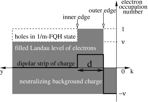
FIG. 1.: Schematic electron-occupation-number profile at the edge of a fractional-QH sample for filling factor $\nu=1-1/m$. This picture (see Ref. [13]) is based on the use of particle-hole conjugation (Refs. [20, 21]) to understand the bulk $\nu=1-1/m$ fractional QH effect. The states are most conveniently described in terms of holes in a filled Landau level. Two fractional-QH strips are formed by the holes: an inner strip with filling factor $\nu^{\text{(i)}}=1-\nu\equiv 1/m$ and an outer strip with filling factor $\nu^{\text{(o)}}=1$. The two strips are separated by a distance $d$. The abscissa is the wave vector $k$ parallel to the edge. In the Landau gauge, a state having wave vector $k$ is localized at a position $y$ perpendicular to the edge which is proportional to $k$. Here, we measure $y$ from the physical boundary of the sample inwards. If the 2D electron system is placed in a coplanar neutralizing background charge with a sharp edge, the total charge density will be negative between inner and outer hole strips and positive inside the outer hole strip. The schematic illustration of the resulting dipolar strip of charge is unrealistic in its depiction of the variation of charge density across the edge. The density profiles at the edges of both hole strips vary on a magnetic-length scale. Accounting for this in our calculations requires only the introduction of appropriate form factors.

FIG. 2.: For a quantum-Hall system with bulk filling factor $\nu=1-1/m$, the ground-state charge-density profile at a sharp edge will have the dipolar strip that is illustrated schematically in Fig. 1. However, at any point along the edge, the 1D charge density in the ground state, obtained by integrating the 2D charge density along the coordinate perpendicular to the edge, is zero. At long wave lengths, parameters of the generalized Tomonaga-Luttinger model for the edge are dominated by the long-range interactions between 1D charge-density fluctuations. On the other hand, the chiral-phonon-mode velocity is determined by smaller residual interactions. In order to determine these accurately, we introduce a fictitious model system in which the edge of the background charge is adjusted to maintain zero 1D charge density at each point along the edge. For example, when a hole is added at the inner edge [(a)], the background charge is reduced by moving its outer edge as illustrated in (b). Similarly, when the outer edge is moved outward, the background edge is also moved outward. (See text.) Here we measure densities in units of $1/(2\pi\ell^{2})$.

FIG. 3.: The process we consider to calculate the parameters $d$ and $v_{\text{J}}$. We consider configurations in which the holes have phase-separated into two incompressible strips as in the ground state at filling factor $\nu=1-1/m$, but allow the separation $y^{\text{(i)}}_{\text{ini}}-y^{\text{(o)}}_{\text{ini}}$ of the two strips to differ from $d$ ($\equiv$ the strip separation in the ground state). We imagine then that a hole is transferred from the edge of the inner strip to the edge of the outer strip, preserving the 1D-local neutrality of the reference state. No adjustment of the background is necessary, and the overall shape of the 1D density profile is similar to its shape in the ground state. We are able to extract the values of $d$ and $v_{\text{J}}$ from the energy change produced by the hole transfer.

FIG. 4.: Energy balance for the transfer of a hole from the inner edge to the outer one (see Fig. 3). The curves are calculated for a filling factor $\nu=2/3$. The electrostatic energy required to transfer the hole (solid curve) is the work performed against the external potential stemming from the dipolar strip of charge; see Fig. 1. Details of its evaluation are given in the appendix. This portion of the energy is linear in the separation $y^{\text{(i)}}_{\text{ini}}-y^{\text{(o)}}_{\text{ini}}$ of the inner and outer edges for separations larger than the magnetic length. The exchange-correlation energy gain is given approximately by $|\zeta(1)|-|\zeta(1/3)|$. Corrections to the simple expression for the exchange-correlation energy gain detailed in the appendix become important at smaller inter-edge distance. The full result for the exchange-correlation energy gain is given by the dashed curve. The point where the two curves cross gives the equilibrium edge separation within our variational two-strip model. The approximations used in our calculation of the exchange-correlation energy are not valid for strip separations much smaller than the magnetic length $\ell$, and the crossing of the curves at the smaller value of $y^{\text{(i)}}_{\text{ini}}-y^{\text{(o)}}_{\text{ini}}$ is unphysical. The other crossing occurs in a regime where our approximations apply. From the point of crossing we conclude that $d\approx 1.7\,\ell$. At this value of $d$, the exchange-correlation energy gain is nearly constant and the electrostatic-energy-cost curve is nearly linear. From its slope we obtain $v_{\text{J}}\approx 0.24\,e^{2}/(\epsilon\hbar)$.

FIG. 5.: External potential for holes. In addition to the electrostatic contribution [dashed curve; cf. Eq. (B22)] resulting from the dipolar strip of charge, there is an additional contribution to the external potential [dot-dashed curve; cf. Eq. (B23)] which is entirely due to particle-hole conjugation in a finite system. This second contribution attracts holes to the physical edge of the sample and is essential for the phase separation into an inner and outer hole strip. The electrostatic potential was calculated for filling factor $\nu=2/3$ and a separation $y^{\text{(i)}}-y^{\text{(o)}}=d_{\text{2/3}}\approx 1.7\,\ell$ of the inner and outer edges.

FIG. 6.: Accounting for the full 2D density profile in our calculation of the Coulomb contribution, $\delta E_{\text{C}}$, to the edge-mode energy requires the introduction of appropriate form factors, $F^{\text{(i)}}(y)$ and $F^{\text{(o)}}(y)$, for the inner and outer hole strips. (See Sec. III A.) As shown in Appendix C, these form factors are related to the derivative of the 2D ground-state density profile in the transverse direction. It is possible to determine $F^{\text{(o)}}(y)$ analytically [dotted curve, see Eq. (C16)] because there are no fluctuations in the occupation numbers for holes in the outer strip which has a filling factor equal to one. The situation is more complicated for the inner hole strip which has a fractional filling factor equal to $1/m$ with $m=3,5,\dots$. As the solid curve, we show the form factor $F^{\text{(i)}}(y)$ for $m=3$ obtained from the ground-state density profile that has been determined numerically in Ref. [39].

REFERENCES

- [1]
- [2] The Quantum Hall Effect, 2nd ed., edited by R. E. Prange and S. M. Girvin (Springer, New York, 1990).
- [3] T. Chakraborty and P. Pietiläinen, The Quantum Hall Effects, 2nd ed. (Springer, Berlin, 1995).
- [4] A. H. MacDonald, in Mesoscopic Quantum Physics, Proceedings of the 1994 Les Houches Summer School, Session LXI, edited by E. Akkermans et al. (Elsevier Science, Amsterdam, 1995), pp. 659–720.
- [5] Edge magnetoplasmons occur quite generally in finite 2D electron systems that are subject to perpendicular magnetic fields; for a review and extensive references, see V. A. Volkov and S. A. Mikhailov, in Landau Level Spectroscopy, edited by G. Landwehr and E. I. Rashba (Elsevier, Amsterdam, 1991), pp. 855–907.
- [6] For a smooth confining potential (i.e., a potential that varies slowly on a microscopic length scale), electrostatics most dominantly determines the structure of the edge; see, for example, D. B. Chklovskii, B. I. Shklovskii, and L. I. Glazman, Phys. Rev. B 46, 4026 (1992). The simple 1D models discussed in our work do not apply in this case. Most likely, the edge is smooth in most quantum Hall systems. The cleaved-edge overgrowth technique [L. N. Pfeiffer et al., Appl. Phys. Lett. 56, 1697 (1990)] offers one method which can be used to create QH samples with sharp edges. For recent work on microscopic models describing the opposite limit of a smooth edge, see, e.g., S. Conti and G. Vignale, Phys. Rev. B 54, R14309 (1996); Physica E 1, 101 (1997); J. H. Han and D. J. Thouless, Phys. Rev. B 55, R1926 (1997); J. H. Han, Phys. Rev. B 56, 15806 (1997).
- [7] J. Voit, Rep. Prog. Phys. 57, 977 (1994).
- [8] B. I. Halperin, Phys. Rev. B 25, 2185 (1982).
- [9] X. G. Wen, Int. J. Mod. Phys. B 6, 1711 (1992), and references cited therein.
- [10] X. G. Wen, Adv. Phys. 44, 405 (1995).
- [11] A. H. MacDonald, S. R. Yang, and M. D. Johnson, Aust. J. Phys. 46, 345 (1993).
- [12] C. de C. Chamon and X. G. Wen, Phys. Rev. B 49, 8227 (1994).
- [13] A. H. MacDonald, Phys. Rev. Lett. 64, 220 (1990).
- [14] C. L. Kane and M. P. A. Fisher, in Perspectives in the Quantum Hall Effects, edited by S. Das Sarma and A. Pinczuk (Wiley, New York, 1997), pp. 109–159.
- [15] R. C. Ashoori et al., Phys. Rev. B 45, 3894 (1992).
- [16] Original works are, e.g., S. Tomonaga, Prog. Theor. Phys. 5, 544 (1950); J. Luttinger, J. Math. Phys. 4, 1154 (1963); D. C. Mattis and E. H. Lieb, J. Math. Phys. 6, 304 (1965). For a recent review and additional references, see Ref. [7]. Note that the effective 1D model describing a QH edge is different from a generic TL model in that the left-going and right-going branches are nonequivalent because they represent chiral 1D electron gases that form the boundary of QH systems at different filling factor.
- [17] The original work by V. P. Silin is published in Zh. Èksp. Teor. Fiz. 33, 495 (1957) [Sov. Phys. JETP 6, 387 (1958)]. For a review, see, e.g., D. Pines and P. Nozières, The Theory of Quantum Liquids (Addison-Wesley, Reading, MA, 1989), Vol. I.
- [18] U. Zülicke, R. Bluhm, V. A. Kostelecký, and A. H. MacDonald, Phys. Rev. B 55, 9800 (1997).
- [19] We use the convention that the outer mode is right-going and the inner mode is left-going. This corresponds to choosing a sign for the transverse external magnetic field. The direction of propagation for the EMP mode is given by the rule for classical cross drift. [See, e.g., J. D. Jackson, Classical Electrodynamics, Second ed. (Wiley, New York, 1975), p. 582.]
- [20] S. M. Girvin, Phys. Rev. B 29, 6012 (1984).
- [21] A. H. MacDonald and D. B. Murray, Phys. Rev. B 32, 2707 (1985).
- [22] J. J. Palacios and A. H. MacDonald, Phys. Rev. Lett. 76, 118 (1996).
- [23] A. H. MacDonald, Brazilian J. Phys. 26, 43 (1996).
- [24] M. D. Johnson, in High Magnetic Fields in the Physics of Semiconductors, edited by D. Heiman (World Scientific, 1995).
- [25] M. D. Johnson and A. H. MacDonald, Phys. Rev. Lett. 67, 2060 (1991).
- [26] J. M. Kinaret et al., Phys. Rev. B 45, 9489 (1992); ibid. 46, 4681 (1992).
- [27] D. Yoshioka, J. Phys. Soc. Jpn. 62, 839 (1993).
- [28] M. Greiter, Phys. Lett. B 336, 48 (1994).
- [29] Y. Meir, Phys. Rev. Lett. 72, 2624 (1994).
- [30] Here and in the following, is the coordinate which the outermost lowest-Landau-level orbital from the inner strip is centered at. Likewise, the orbital with the smallest wave-vector label among the states occupied by holes from the outer hole strip is centered at .
- [31] U. Zülicke and A. H. MacDonald, Phys. Rev. B 54, 16813 (1996).
- [32] A. H. MacDonald and M. D. Johnson, Phys. Rev. Lett. 70, 3107 (1993).
- [33] M. Stone, H. W. Wyld, and R. L. Schult, Phys. Rev. B 45, 14156 (1992).
- [34] The appropriate value of depends on the specific sample geometry in which the 2D electron system is realized and need not be the bulk-semiconductor dielectric constant . Only if the wave length of the excitations of interest is much smaller than the distance of the 2D electron system to the surface of the (3D) semiconductor sample, . The opposite limit is, however, more typical. We therefore use for the numerical estimates presented in this work.
- [35] The energy per particle for fractional-QH systems at filling factor has been calculated for various fillings by exact numerical diagonalization,[39, 41, 42] Monte-Carlo methods,[43, 39] and using the variational wave function proposed by Laughlin.[44] To determine the parameter , we need to know and . Simply from a calculation of the exchange energy for an electron at the edge of a filling-factor-one QH strip, we know[45] that . In our numerical calculations for the case of , we used .
- [36] U. Zülicke and A. H. MacDonald, unpublished.
- [37] I. L. Aleiner and L. I. Glazman, Phys. Rev. Lett. 72, 2935 (1994).
- [38] S. Mitra and A. H. MacDonald, Phys. Rev. B 48, 2005 (1993).
- [39] N. Datta, R. Morf, and R. Ferrari, Phys. Rev. B 53, 10906 (1996).
- [40] M. Stone, Phys. Rev. B 42, 8399 (1990).
- [41] D. Yoshioka, Phys. Rev. B 29, 6833 (1984).
- [42] M. Kasner and W. Apel, Ann. Phys. (Leipzig) 3, 433 (1994).
- [43] R. Morf and B. I. Halperin, Phys. Rev. B 33, 2221 (1986).
- [44] R. B. Laughlin, Phys. Rev. Lett. 51, 1395 (1983).
- [45] A. H. MacDonald and S. M. Girvin, Phys. Rev. B 34, 5639 (1986).
- [46]