The Two-Dimensional $S=1$ Quantum Heisenberg Antiferromagnet at Finite Temperatures

Recently, field theoretical predictions ${}^{\hbox{\immediate{\bf{?}},\penalty 1000\hskip 0.91003pt plus 0.70004pt minus 0.70004pt{\bf{?}},\penalty 1000\hskip 0.91003pt plus 0.70004pt minus 0.70004pt{\bf{?}})}}$ concerning the correlation length of the square lattice quantum Heisenberg antiferromagnet (QHA) were directly checked by experimental measurements ${}^{\hbox{\immediate{\bf{?}},\penalty 1000\hskip 0.91003pt plus 0.70004pt minus 0.70004pt{\bf{?}})}}$ and several quantum Monte Carlo (QMC) simulations .${}^{\hbox{\immediate{\bf{?}},\penalty 1000\hskip 0.91003pt plus 0.70004pt minus 0.70004pt{\bf{?}},\penalty 1000\hskip 0.91003pt plus 0.70004pt minus 0.70004pt{\bf{?}},\penalty 1000\hskip 0.91003pt plus 0.70004pt minus 0.70004pt{\bf{?}})}}$ While in the case of spin $S=1/2$ the validity of the predictions seemed supported by experiments, in the case of $S=1$, experimental measurements for both ${\rm La}_{2}{\rm NiO}_{4}$ ${}^{\hbox{\immediate{?})}}$ and ${\rm K}_{2}{\rm NiF}_{4}$ ${}^{\hbox{\immediate{?})}}$ turned out to be inconsistent with the theoretical predictions.

The inconsistencies were explained by noting that the theoretical low temperature expression is valid for the temperatures of the $S=1/2$ experiments, but not valid in the temperature regime of the $S=1$ experiments. While a number of simulations have been performed for $S=1/2$, only a high temperature series expansion calculation ${}^{\hbox{\immediate{\bf{?}})}}$ and an effective high temperature theory (PQSCHA) ${}^{\hbox{\immediate{\bf{?}},\penalty 1000\hskip 0.91003pt plus 0.70004pt minus 0.70004pt{\bf{?}},\penalty 1000\hskip 0.91003pt plus 0.70004pt minus 0.70004pt{\bf{?}})}}$ are available for $S=1$ in the experimentally relevant temperature range. In this paper, we compute the correlation length and other thermal averages for the $S=1$ QHA on a square lattice using the quantum Monte Carlo loop algorithm ${}^{\hbox{\immediate{\bf{?}})}}$ generalized to larger spins .${}^{\hbox{\immediate{\bf{?}},\penalty 1000\hskip 0.91003pt plus 0.70004pt minus 0.70004pt{\bf{?}},\penalty 1000\hskip 0.91003pt plus 0.70004pt minus 0.70004pt{\bf{?}})}}$ This algorithm was implemented in continuous imaginary-time representation ${}^{\hbox{\immediate{\bf{?}})}}$ to eliminate the systematic error due to Suzuki-Trotter discretization of path integrals.

When implemented in continuous imaginary time, the probability for the graph assignment in the cluster algorithms for larger spins becomes much simpler than the original discrete time version  ,${}^{\hbox{\immediate{?},\penalty 1000\hskip 0.91003pt plus 0.70004pt minus 0.70004pt{?})}}$ although the idea is essentially the same. As in the case of discrete time, we first extend the Hilbert space by expressing each spin operator by a sum of $2S$ Pauli spins:

$$S_{i}=\frac{1}{2}\sum_{\mu=1}^{2S}\sigma_{i\mu}.$$ (1)

We therefore consider $(2SN)$ vertical lines along the imaginary time axis, each specified by two indices $(i\mu)$, where $N$ is the total number of original spins. Since there are unphysical states in the new Hilbert space in which some of the spins have magnitude less than $S$, we must eliminate such states by applying projection operators. Here we use a representation where $z$-spin components are diagonalized. Our procedure for the graph assignment is as follows. For each pair of neighboring world lines and for each uninterrupted time interval during which spins on these world lines are antiparallel, we generate “cuts” of worldlines with probability density $J/2$. At each cut, we reconnect pairwise the four end points created by the cut by two horizontal segments (Fig. 1). The application of the above-mentioned projection operator for a site is realized by choosing an appropriate boundary condition in the temporal direction. If the spin values $(\sigma_{(i\mu)}^{z}(\tau))$ are the same at the four end points, $(i1)$ and $(i2)$ at $\tau=\beta$ and at $\tau=0$, we choose a straight connection (connecting $(i1)$ at $\tau=\beta$ to $(i1)$ at $\tau=0$) and a cross connection (connecting $(i1)$ at $\tau=\beta$ to $(i2)$ at $\tau=0$) with equal probability. Otherwise, we choose the unique method for connecting these four points pairwise so that the spin value at each connection point is continuous. Thus, we form many loops which are to be flipped with probability 1/2. This algorithm turns out to be more efficient than its discrete version.

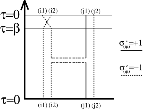
Fig.  1: A cut and two horizontal segments. The two types of boundary condition in temporal direction are also illustrated.

Using chiral perturbation theory, Hasenfratz and Niedermayer(HN) ${}^{\hbox{\immediate{?})}}$ obtained the temperature dependence of the correlation length up to two-loop order for an arbitrary magnitude of spin:

$$\xi_{HN}=\frac{e}{8}\frac{\hbar c}{2\pi\rho_{s}}\exp\left(\frac{1}{t}\right)\times\left[1-\frac{t}{2}+{\cal O}\left(t^{2}\right)\right],$$ (2)

where $t\equiv k_{\rm B}T/2\pi\rho_{S}$. The dependence on the magnitude of the spin $S$ is only implicit through the $S$-dependence of the the spin-stiffness constant $\rho_{s}$, and the spin wave velocity $c$. For $S=1/2$, the spin wave theory (SWT) ${}^{\hbox{\immediate{\bf{?}})}}$ values for $\rho_{s}$ and $c$ were observed to be close to the QMC estimates. As SWT is better for larger spins, we can confidently use the SWT values for $S=1$ in the following with $2\pi\rho_{s}=5.461J$ and $\hbar c=3.067J$. These values agree with the result of a series expansion around the Ising limit, within statistical errors smaller than 1%.

Equation (2) is valid in the renormalized classical regime where

$$t\ll 1.$$ (3)

An additional constraint on the temperature comes from the cutoff of the quantum fluctuations in the effective field theory once the extension in the imaginary time direction $\beta$ becomes smaller than the lattice spacing $a/\hbar c$:

$$t\ll{\hbar c\over 2\pi\rho_{s}a}\approx{\sqrt{2}\over\pi}{1\over S}\left(1+{0.196\over S}\right).$$ (4)

The approximation in the last term on the right hand side is again the leading order SWT result.

In the case of $S=1/2$ QHA, it was found by QMC simulations that eq. (2) is valid only at very large correlation lengths ${}^{\hbox{\immediate{?},\penalty 1000\hskip 0.91003pt plus 0.70004pt minus 0.70004pt{?})}}$ of the order of 100 lattice spacings or larger. In the experimentally relevant temperature regime the deviations, while clearly visible in the QMC simulations, are however smaller than the experimental errors. Thus, the theory and experiment agree for $S=1/2$.

The large discrepancies observed for $S=1$ ${}^{\hbox{\immediate{?},\penalty 1000\hskip 0.91003pt plus 0.70004pt minus 0.70004pt{?})}}$ are somewhat counterintuitive, since the theory based on a spin-wave picture should be better for larger spins. However, this is not very surprising since eq. (2) reflects the quantum nature of the system and therefore eq. (2) applies only if eq. (4) is satisfied. The region determined by eq. (4) should be smaller for systems closer to the classical system. Therefore, since larger spins are more classical as noted previously in refs. ?, ?, ?, ?, the validity of eq. (2) is restricted to even larger correlation lengths than for $S=1/2$, much larger than accessible in experiments.

As the analytic low temperature form is not valid in the experimentally accessible temperature regime, we performed QMC simulations over the temperature range $t\geq 0.18$ ($k_{\rm B}T\geq J$) in order to compare the experimental data ${}^{\hbox{\immediate{?})}}$ with the $S=1$ QHA. The second moment correlation length $\xi_{L}$ on a finite system of size $L$ was determined from the static structure factor $S_{L}({\mbox{\boldmath$q$}})$ in the vicinity of ${\mbox{\boldmath$Q$}}=(\pi,\pi)$ .${}^{\hbox{\immediate{\bf{?}})}}$ The $\xi_{L}$ is calculated as follows.

$$\xi^{-2}_{L}\equiv f(2\pi/L,0)+f(0,2\pi/L)-f(2\pi/L,2\pi/L),$$ (5)

where

$$f({\mbox{\boldmath$q$}})\equiv 4\sin^{2}\left(\frac{{\mbox{\boldmath$q$}}}{2}\right)\left(1-\frac{S({\mbox{\boldmath$Q$}}+{\mbox{\boldmath$q$}})}{S({\mbox{\boldmath$Q$}})}\right)^{-1}.$$ (6)

This estimator for the correlation length (of a finite system) should be correct up to the fourth order in $2\pi/L$. We use improved estimators to reduce statical errors. For a given temperature $T$, when the lattice size $L$ is sufficiently large, $\xi_{L}$ converges to a size-independent value $\xi(T)$, which we regard as the infinite-size limit. We find that the convergence is achieved to the accuracy determined by the present statistical error when the condition $L\geq 7\xi_{L}$ is satisfied. All the following results are obtained under this condition. For each simulation we have performed $10^{6}$ sweeps, after $10^{4}$ thermalization sweeps.

A selection of our results for the correlation length $\xi$, the staggered structure factor $S(\pi,\pi)$ and the uniform susceptibility $\chi$ are summarized in Table I. In Fig. 2, we plot our QMC results for the correlation length together with the experimental data ${}^{\hbox{\immediate{?})}}$ and theoretical predictions based on eq. (2). Our present estimates are in rough agreement with experimental measurements. Greven et al. ${}^{\hbox{\immediate{?})}}$ and Nakajima et al. ${}^{\hbox{\immediate{?})}}$ have additionally proposed to include the effects of a small Ising anisotropy using a mean-field type correction to the theoretical isotropic results. This correction (eq. (7) of ref. ?) however makes the agreement worse, as can be seen from Fig. 2.

Compared to theoretical predictions we find that the data deviate strongly from the low temperature formula of eq. (2). The effective PQSCHA approximation ,${}^{\hbox{\immediate{?},\penalty 1000\hskip 0.91003pt plus 0.70004pt minus 0.70004pt{?},\penalty 1000\hskip 0.91003pt plus 0.70004pt minus 0.70004pt{?})}}$ which is an effective high temperature theory, however agrees well with the QMC results much better than for $S=1/2$ .${}^{\hbox{\immediate{?},\penalty 1000\hskip 0.91003pt plus 0.70004pt minus 0.70004pt{?},\penalty 1000\hskip 0.91003pt plus 0.70004pt minus 0.70004pt{?},\penalty 1000\hskip 0.91003pt plus 0.70004pt minus 0.70004pt{?})}}$

Table  I: Correlation length $\xi$, magnetic structure factor $S(\pi,\pi)$ and uniform susceptibility $\chi$ as a function of temperature $t=k_{\rm B}T/2\pi\rho_{s}$.

$J/k_{\rm B}T$	$t$	$L$	$\xi$			$S(\pi,\pi)$			$\chi$
0.10	1.83	20	0	.	298(5)	0	.	8915(1)	0	.	051579(6)
0.15	1.22	20	0	.	396(5)	1	.	0489(2)	0	.	068503(9)
0.20	0.92	20	0	.	497(5)	1	.	2481(3)	0	.	08118(1)
0.25	0.73	20	0	.	610(5)	1	.	5029(5)	0	.	09038(1)
0.30	0.61	20	0	.	739(5)	1	.	8342(7)	0	.	09687(2)
0.35	0.52	20	0	.	894(6)	2	.	272(1)	0	.	10108(2)
0.40	0.46	20	1	.	079(6)	2	.	854(2)	0	.	10343(2)
0.45	0.41	20	1	.	307(6)	3	.	648(2)	0	.	10435(3)
0.50	0.37	30	1	.	604(3)	4	.	776(1)	0	.	104000(8)
0.55	0.33	30	1	.	982(8)	6	.	392(4)	0	.	10275(2)
0.60	0.31	40	2	.	482(5)	8	.	795(2)	0	.	100756(8)
0.65	0.28	40	3	.	14(1)	12	.	46(1)	0	.	09829(3)
0.70	0.26	50	4	.	06(1)	18	.	25(2)	0	.	09560(2)
0.75	0.24	50	5	.	30(2)	27	.	60(3)	0	.	09275(3)
0.80	0.23	60	7	.	06(2)	43	.	30(5)	0	.	09000(3)
0.85	0.22	80	9	.	52(3)	70	.	03(8)	0	.	08746(3)
0.90	0.20	120	12	.	98(4)	116	.	4(1)	0	.	08516(3)
0.95	0.19	140	17	.	97(5)	198	.	8(3)	0	.	08309(3)
1.00	0.18	200	24	.	94(7)	344	.	0(4)	0	.	08133(2)

Fig.  2: The correlation length $\xi$ as a function of $t=k_{\rm B}T/2\pi\rho_{s}$. Filled squares represent the results of our simulation, the open circles are experimental measurements .${}^{\hbox{\immediate{?})}}$ While the experimental measurements agree roughly with our QMC results, they are incompatible with the QMC results corrected for a small Ising anisotropy (open squares). Compared to analytic calculations, we find that in this temperature range the low-temperature predictions of eq. (2) (dashed line) are not valid. The PQSCHA approximation ,${}^{\hbox{\immediate{?},\penalty 1000\hskip 0.91003pt plus 0.70004pt minus 0.70004pt{?},\penalty 1000\hskip 0.91003pt plus 0.70004pt minus 0.70004pt{?})}}$ however, agrees well with both our data and the experimental measurements.

Another violation of the theoretical predictions ${}^{\hbox{\immediate{?},\penalty 1000\hskip 0.91003pt plus 0.70004pt minus 0.70004pt{?})}}$ was observed in the peak value of the staggered structure factor $S(\pi,\pi)$, which according to the theory ${}^{\hbox{\immediate{?},\penalty 1000\hskip 0.91003pt plus 0.70004pt minus 0.70004pt{?},\penalty 1000\hskip 0.91003pt plus 0.70004pt minus 0.70004pt{\bf{?}})}}$ should scale as

$$S(\pi,\pi)=A2\pi M^{2}\xi^{2}t^{2}(1+Ct).$$ (7)

Here $M$ is the staggered magnetization of the ground state and $A$ and $C$ are universal constants. For spin-1/2 the leading $t^{2}$ form was confirmed by high temperature series .${}^{\hbox{\immediate{?})}}$ Recent QMC data ${}^{\hbox{\immediate{?})}}$ at lower temperatures fit the above form very well in the temperature range $t<3$ with $A\approx 4.0(1)$ and $C\approx 0.5(1)$. However, experiments for both $S=1/2$ and $S=1$ were better described by an empirical law ${}^{\hbox{\immediate{?},\penalty 1000\hskip 0.91003pt plus 0.70004pt minus 0.70004pt{?})}}$

$$S(\pi,\pi)\propto\xi^{2}$$ (8)

over the same temperature range.

We applied a $\chi^{2}$ analysis to check the consistency of the spin-1 data. Good fits were obtained for $t<0.28$, with $\chi^{2}\sim 1$ when we allow $C$ to vary, and $\chi^{2}\sim 2$ with a fixed $C=0.5$. The universal constant $A$ was determined to be $A=4.1(1)$ and $A=4.5(1)$ , similar to the values obtained for $S=1/2$. The discrepancies between the fits are non-universal effects caused by the rather high temperatures.

Comparison of our data with the experiments is shown in Fig. 3 and we can see that for low temperatures the experimental data are consistent with the QMC results and eq. (7). The discrepancies that lead refs. ? and ? to predict eq. (8) occur at higher temperatures where the experimental data has large error bars. In view of the precision of our QMC results and the large errors of the experimental results we suspect that, contrary to the suggestion of refs. ? and ?, the deviations from eq. (7) are due to uncertainties in the experimental measurements.

Fig.  3: The ratio of structure factor peak value and square of the correlation length $S(\pi,\pi)/\xi^{2}$ as a function of temperature. Solid circles represent the QMC measurements and open squares the experimental measurements. They agree at low temperatures, but differ at higher temperatures. The solid line is a fit of the QMC data to the theoretical low-temperature prediction.

Finally, we present in Fig. 4 the uniform susceptibility for $S=1/2$ together with previously published $S=1/2$ results. First we note that, as expected, the asymptotic low temperature behavior of the renormalized classical regime

$$\chi={2\rho_{s}\over 3}\left({g\mu_{B}\over\hbar c}\right)^{2}(1+t+t^{2})$$ (9)

sets in at lower temperatures for $S=1$ than for $S=1/2$.

It was discovered that for $S=1/2$, the uniform susceptibility is the only quantity for which a clear crossover to quantum critical behavior ${}^{\hbox{\immediate{?})}}$ can be observed at intermediate temperatures $t\sim 1/3$. The uniform susceptibility in the quantum critical regime is

$$\chi=\chi_{\perp}+BT\left({g\mu_{B}\over\hbar c}\right)^{2},$$ (10)

with a universal slope $B\approx 0.26(1)$ .${}^{\hbox{\immediate{?},\penalty 1000\hskip 0.91003pt plus 0.70004pt minus 0.70004pt{\bf{?}},\penalty 1000\hskip 0.91003pt plus 0.70004pt minus 0.70004pt{\bf{?}})}}$ For $S=1$ however, as discussed above, non-universal corrections become important at lower temperatures. No quantum critical behavior was thus expected for $S=1.$ We can see in Fig. 4 that the uniform susceptibility for $S=1$ deviates from its universal quantum critical behavior at intermediate temperatures. Its slope is however still surprisingly close to the quantum critical one, indicating that the non-universal corrections are still not very large for $S=1$.

Fig.  4: The uniform susceptibility $\chi$ as a function of temperature $t$ for both spin $S=1$ and spin $S=1/2$ (taken from ref. ?). The solid line is the predicted low temperature form of the renormalized classical regime. The dashed lines have the universal slope expected for the quantum critical regime. As expected, contrary to $S=1/2$, no extended quantum critical regime exists for $S=1$. However the slope is close to the quantum critical value as non-universal corrections are still small for $S=1$.

In summary, we have simulated the spin $S=1$ quantum Heisenberg antiferromagnet on a square lattice in the experimentally relevant temperature regime $k_{\rm B}T\sim J$. We find a better agreement between the Heisenberg model and experimental data than is expected from the low temperature theory. However, in view of the existing small discrepancies it may be necessary to perform simulations on a model with small anisotropies in the exchange interactions, and to critically check the data analysis of the experiments.

References

- [1] S. Chakravarty, B. I. Halperin and D. R. Nelson: Phys. Rev. B 39 (1989) 2344.
- [2] P. Hasenfratz and F. Niedermayer: Phys. Lett. B 268 (1991) 231.
- [3] A. V. Chubukov, S. Sachdev and J. Ye: Phys. Rev. B 49 (1994) 11919.
- [4] K. Nakajima, K. Yamada, S. Hosoya, Y. Endoh, M. Greven and R. J. Birgeneau: Z. Phys. B 96 (1995) 479.
- [5] M. Greven, R. J. Birgeneau, Y. Endoh, M. A. Kastner, M. Matsuda and G. Shirane: Z. Phys. B 96 (1995) 465.
- [6] M. S. Makivic and H.-Q. Ding: Phys. Rev. B 43 (1991) 3562.
- [7] J.-K. Kim, D. P. Landau and M. Troyer: Phys. Rev. Lett. 79 (1997) 1583.
- [8] B. B. Beard, R. J. Birgeneau, M. Greven and U.-J. Wiese: Phys. Rev. Lett. 80 (1998) 1742.
- [9] J.-K. Kim and M. Troyer: Phys. Rev. Lett. 80 (1998) in press.
- [10] N. Elstner, A. Sokal, R. R. P. Singh, M. Greven and R. J. Birgeneau: Phys. Rev. Lett. 75 (1995) 938.
- [11] A. Cuccoli, V. Tognetti, R. Vaia and P. Verrucchi: Phys. Rev. Lett. 77 (1996) 3439.
- [12] A. Cuccoli, V. Tognetti, R. Vaia and P. Verrucchi: Phys. Rev. Lett. 79 (1997) 1584.
- [13] A. Cuccoli, V. Tognetti, R. Vaia and P. Verrucchi: Phys. Rev. B 56 (1997) 14456.
- [14] H. G. Evertz, M. Marcu and G. Lana: Phys. Rev. Lett. 70 (1993) 875.
- [15] N. Kawashima and J. E. Gubernatis: J. Stat. Phys. 80 (1995) 169.
- [16] N. Kawashima: J. Stat. Phys. 82 (1996) 131.
- [17] N. Kawashima and J. E. Gubernatis: Phys. Rev. Lett. 73 (1994) 1295.
- [18] B. B. Beard and U. J. Wiese: Phys. Rev. Lett. 77 (1996) 5130.
- [19] C. J. Hammer, Z. Weihong and J. Oitmaa: Phys. Rev. B 50 (1994) 6877.
- [20] G. A. Baker, Jr and N. Kawashima: Phys. Rev. Lett. 75 (1995) 994.
- [21] A. Chubukov: private communications.
- [22] M. Troyer, M. Imada and K. Ueda: J. Phys. Soc. Jpn. 66 (1997) 2957.
- [23] M. Troyer and M. Imada in Computer Simulations in Condensed Matter Physics X, ed. D. P. Landau et al., (Springer Verlag, Heidelberg, 1997).