[

Spin-Blockade in Single and Double Quantum Dots in Magnetic Fields:
a Correlation Effect

Abstract

The total spin of correlated electrons in a quantum dot changes with magnetic field and this effect is generally linked to the change in the total angular momentum from one magic number to another, which can be understood in terms of an ‘electron molecule’ picture for strong fields. Here we propose to exploit this fact to realize a spin blockade, i.e., electrons are prohibited to tunnel at specific values of the magnetic field. The spin-blockade regions have been obtained by calculating both the ground and excited states. In double dots the spin-blockade condition is found to be less stringent than in single dots.

]

The Coulomb blockade is one of the highlights in the transport properties of mesoscopic systems such as quantum dots. This is a combined effect of the discreteness of energy levels and the electron-electron interaction (charging energy). Now, it has recently been suggested that, if the total spins of the ground state of $N$ and $(N-1)$-electrons differ by more than 1/2, the dot is blocked with the corresponding peak in the conductance missing at zero temperature. This is called the spin-blockade [1, 2] and has been studied theoretically for weak electron interaction regimes. There the Hund’s coupling picture, in which electrons are accommodated in one-electron states with high spins for degenerate states, tends not to realize the spin-blockade condition, so that some modifications such as an anharmonicity in the confinement potential [3] have to be introduced.

When quantum dots are placed in strong magnetic fields, the ground states are known to change dramatically into the magic-number states [4, 5]. This comes from the electron correlation effect, since the magic numbers for the total angular momentum arise from a combined effect of the electron correlation and Pauli’s principle, persisting even when the Zeeman energy is completely ignored. The total angular momentum of the ground state jumps from one magic number to another as the magnetic field $B$ is varied.

An important hint that electron correlation is really at work is the fact that the total spin ($S$), where $\mbox{\boldmath$S$}^{2}=S(S+1)$, of the ground state, which dominates how the electrons correlate, changes wildly as shown in Fig. 1. This happens when the typical Coulomb energy is much greater than the single-electron level spacing, where electron molecule are formed. In this sense this is genuinely an electron-correlation effect — electron correlation has been known to dominate the spin states in ordinary correlated electron systems such as the Hubbard model, but the present case is a peculiar manifestation in strong magnetic fields.

In the present paper we propose to utilize this electron correlation effect to realize a spin blockade. We have numerically studied the ground and excited states of single dots that contain three or four electrons with a parabolic confinement potential and find that the spin blockade should indeed be observed. Physically, a key observation starts from the fact that the correlated electron states in the dot may be thought of as ‘electron molecules’[6], which in turn enables us to interpret[7] the spin wavefunctions taking part in the spin blockade as spin configurations in molecules, which include the resonating valence bond (RVB) states, that are usually invoked for lattice fermions. We further show that the spin-blockade condition is easier to satisfy in double dots which can be tuned by controlling the layer separation and the strength of the interlayer tunneling.

So let us start with looking at the total angular momentum ($L$) of 2D electrons confined in a quantum dot in a magnetic field , which has a one-to-one correspondence with the spatial extent ($\propto\sqrt{L}$) of the wavefunction. Thus the presence of magic $L$ values signifies that the total Coulombic energy of the interacting electrons, although roughly a decreasing function of $L$ as the electrons move further apart for larger $L$, is not a smooth function of the size of the wavefunction, so that jumps in $L$ are accompanied by jumps in the size of the wave function [8, 9]. For example, the total angular momentum $L$ of three spin-polarized electrons changes $3\rightarrow 6\rightarrow 9\rightarrow\dots$ with increasing magnetic field.

Recently one of the authors has explained this as an effect of correlation in the electron configuration, where Pauli’s exclusion principle dictates group-theoretically the manner in which the quantum numbers should appear [6]. There, the picture of the ‘electron molecule’, in which the electrons with a specific configuration (triangle for three electrons, square for four, etc) rotating as a whole has turned out to be surprisingly accurate. This continues to be the case for larger numbers of electrons [10].

When one considers the spin degrees of freedom, the magic $L$ values are linked with the total spin. This is already apparent in the first numerical study of spin dependent correlation in quantum dots  [11]. These molecules are characterized by a quantum number, $k_{s}$, where the spin wave function $\Psi_{\rm spin}$ is transformed to ${\rm exp}(-2\pi k_{s}i/m)\Psi_{\rm spin}$ under the rotation of $2\pi/m$ for an $m-$fold symmetric molecule. Then the criterion for the magic number, modulo $m$, reads $L+k_{s}\equiv 0(m/2)$ for $m$ odd (even).

To actually obtain the spin states numerically for different numbers of electrons, let us consider single GaAs quantum dots with three or four electrons in a parabolic potential. The electron motion is assumed to be completely two dimensional. The Hamiltonian for a single dot is ${\cal H}={\cal H}_{\rm s}+{\cal H}_{\rm C}$, where

$${\cal H}_{\rm s}=\sum_{n}\sum_{\ell}\sum_{\sigma}\varepsilon_{n\ell\sigma}c_{n\ell\sigma}^{{\dagger}}c_{n\ell\sigma},$$ (1)

is the single-electron part, while

$${\cal H}_{\rm C} = \frac{1}{2}\sum_{n_{1}\sim n_{4}}\sum_{\ell_{1}\sim\ell_{4}}\sum_{\sigma_{1}\sim\sigma_{4}}$$ (4)

$$\mbox{\ }\langle n_{1}\ell_{1}\sigma_{1},n_{2}\ell_{2}\sigma_{2}|\frac{e^{2}}{\epsilon|{\bf r}_{1}-{\bf r}_{2}|}|n_{3}\ell_{3}\sigma_{3},n_{4}\ell_{4}\sigma_{4}\rangle$$

$$\times c_{n_{1}\ell_{1}\sigma_{1}}^{{\dagger}}c_{n_{2}\ell_{2}\sigma_{2}}^{{\dagger}}c_{n_{4}\ell_{4}\sigma_{4}}c_{n_{3}\ell_{3}\sigma_{3}}.$$

represents the Coulomb interaction. Here the Hamiltonian is written in second quantized form in a Fock-Darwin [12] basis, and $\varepsilon_{n\ell\sigma}$$=$$(2n+1+|\ell|)$$\hbar$ $(\omega_{c}^{2}/4+\omega_{0}^{2})^{1/2}$$-\ell\hbar\omega_{c}/2$$-g^{*}\mu_{{}_{B}}Bs_{z}$. The dielectric constant is $\epsilon$, $\hbar\omega_{0}$ represents the strength of the parabolic confinement potential, $\omega_{c}=eB/m^{*}c$ is the cyclotron frequency, $m^{*}$ is the effective mass, $\mu_{{}_{B}}$ is the Bohr magneton, $g^{*}$ is the effective $g$-factor and $s_{z}$ is $z$-component of the spin of a single electron.

We use the confinement potential $\hbar\omega_{0}=6.0$ meV. This is a little larger than usually estimated values $(2\sim 4$ meV) and is deliberately chosen to reproduce the addition energy spectrum [13]. The fact that calculations with a $1/r$ interaction require a larger confinement energy to reproduce experimental results is considered to be a consequence of the modification of the interaction potential in real dots [14].

In our numerical calculations we have used enough states (including higher Landau levels) in the basis to ensure convergence of the ground-state energy within $0.1\%$. Three lowest excited states are also calculated for each value of $B$, which turn out to be the lowest-energy states having different angular momenta in the present case. Excited states are also obtained with a typical accuracy of $<0.1\%$ for an $N=3$ single dot at $B=5$ T.

The total angular momentum, and the total spin of the ground state for three- and four-electron systems plotted in Fig. 1, we can see how the magic $L$ values go hand in hand with $S(N)$ for $N$ electrons, where $\mbox{\boldmath$S$}^{2}=S(S+1)$ while the $z$ component of $S$ is aligned to $B$: As the magnetic field increase, the ground state changes as $(L,S)=(1,1/2)\rightarrow(2,1/2)\rightarrow(3,3/2)$ for $N=3$, $(L,S)=(0,1)\rightarrow(2,0)\rightarrow(3,1)\rightarrow(4,0)\rightarrow(5,1)\rightarrow(6,2)$ for $N=4$.

If we then plot the difference in the total spin, $S(4)-S(3)$, against the magnetic field in the bottom panel of Fig. 2, the spin blockade condition,

$$|S(N)-S(N-1)|>\frac{1}{2},$$ (5)

is indeed fulfilled: $S$ jumps from 3/2 to 0 in the region $4.96<B<5.18$ T.

From the magic-number criterion the state with $(L=2+4\times{\rm integer})$ has to have the quantum number $k_{s}=0$, while the $(L=4\times{\rm integer})$ state $k_{s}=2$ for $N=4$. We can make an intriguing identification, by looking at the spin density correlation function, that $(L,S)=(2,0)$ is an ${\rm RVB}^{-}$ state while $(4,0)$ is an ${\rm RVB}^{+}$, where the RVB’s are defined, for a four-site cluster, as

RVB^-: (7)

$$=|^{\uparrow\uparrow}_{\downarrow\downarrow}\rangle\!+\!|^{\downarrow\downarrow}_{\uparrow\uparrow}\rangle\!+\!|^{\uparrow\downarrow}_{\uparrow\downarrow}\rangle\!+\!|^{\downarrow\uparrow}_{\downarrow\uparrow}\rangle\!-2\!\left[|^{\downarrow\uparrow}_{\uparrow\downarrow}\rangle\!+\!|^{\uparrow\downarrow}_{\downarrow\uparrow}\rangle\right],$$

RVB⁺: (9)

$$=|^{\uparrow\uparrow}_{\downarrow\downarrow}\rangle+|^{\downarrow\downarrow}_{\uparrow\uparrow}\rangle-|^{\uparrow\downarrow}_{\uparrow\downarrow}\rangle-|^{\downarrow\uparrow}_{\downarrow\uparrow}\rangle,$$

with $\equiv\frac{1}{\sqrt{2}}(|\uparrow\downarrow\rangle-|\downarrow\uparrow\rangle)$ being the spin-singlet pair in the electron molecule. The difference of RVB⁺ from RVB^- is that the former lacks the Néel components (the last two terms in RVB^-) and has the extra phase factor -1 for $\pi/2$ rotation. Although what we have here is totally different from lattice fermion systems such as the Hubbard model for which RVB is usually conceived, the electron-molecule formation has brought about such spin configurations.

FIG. 1.: The total angular momentum and total spin of the ground state for a single quantum dot with $N=3$ (left) or $N=4$ electrons (right). The confinement potential is assumed to be parabolic with $\hbar\omega_{0}=6.0$ meV.

In this region, the conduction, blocked at zero temperature, has to occur through an $S=1$ excited state for $N=4$ at finite temperatures. If the excited states are well separated in energy ($\geq$ 0.1 meV, typical experimental resolution for Coulomb diamonds) from the ground state for both of the $(N-1)-$ electron and $N-$ electron states, the spin blockade should be observed in the Coulomb diamond, which is the differential conductance plotted in the plane of source-drain voltage and gate voltage. We have calculated the three lowest excitation energies and their total spins for the $N=4$ quantum dot in Fig. 2. The lowest excited states for $N=3$ and for $N=4$ both lie about 0.06meV above the ground state around $B=5.1$ T in the spin-blockade region. We can make this separation larger ($\sim$ 0.1 meV) for stronger confinement potentials (e.g., 0.09meV around $B=7.4$ T for $\hbar\omega_{0}=8.0$ meV). Such confinement potentials may be realized in a gated vertical quantum dot [13].

The link between the magic $L$ and total $S$ and subsequent spin blockade appears for other numbers of electrons as well, e.g., between $(L,S)=(2,0)$ state for $N=2$ and $(6,3/2)$ state for $N=3$ for $14.1<B<14.8$ T.

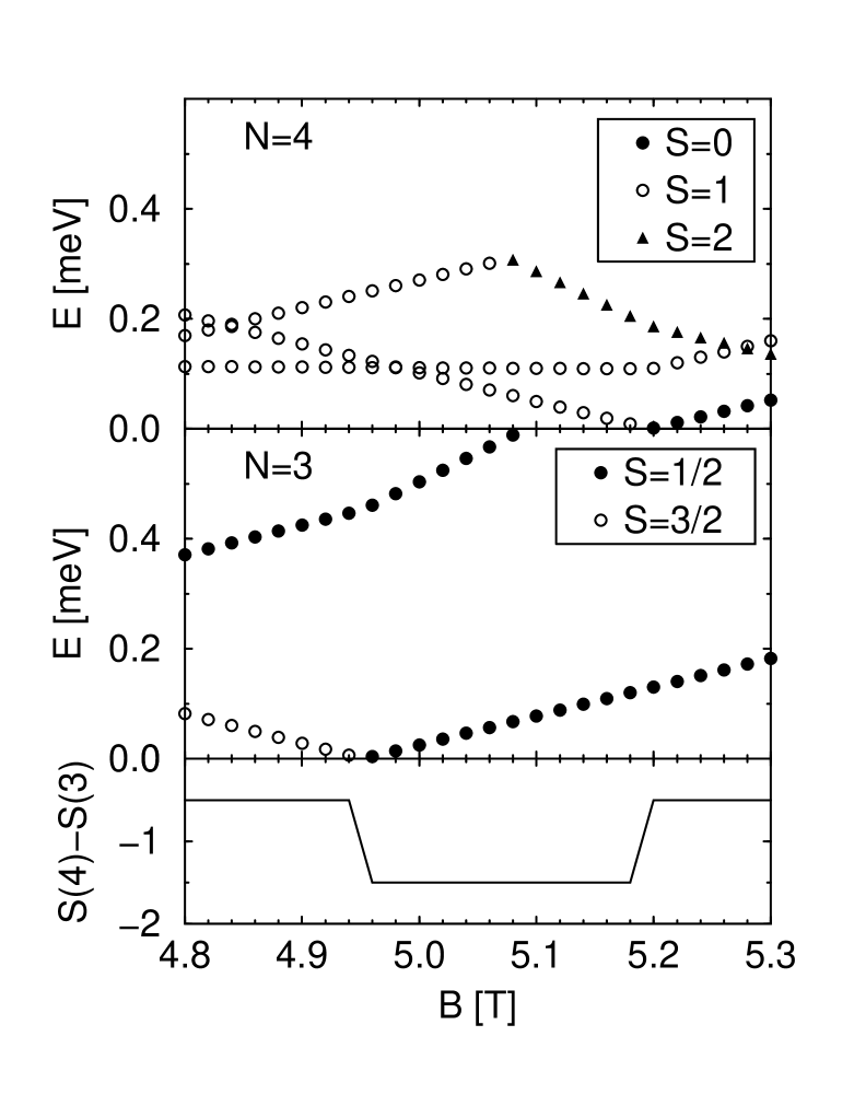
FIG. 2.: Top: Excitation energies for $N=4$ single dot. Middle: The same for $N=3$. Bottom: Difference in the total spin, $S(4)-S(3)$, between the ground state for $N=3,4)$.

Now we move on to the double dots, where dots are separated in the vertical direction with their centers aligned on a common axis. We assume the same confinement potential for the two dots for simplicity. Here electrons are Coulomb-correlated both within each layer and across the two layers, in the presence of the inter-layer tunneling. Recent advances in semiconductor fabrication techniques have enabled fabrication of double dots in vertical, triple-barrier structures on submicron scales [15]. Theory for the double quantum dots has been developed [16, 17, 18, 19, 20, 21], where intriguing features such as magic-number states intrinsic to double dots, or a singlet-to-triplet spin transition for two-electron system have been found [16, 17, 18].

The Hamiltonian now contains the tunneling term,

$${\cal H}_{\rm t}=-\frac{\Delta_{\rm SAS}}{2}\sum_{n}\sum_{\ell}\left(c_{n\ell+}^{{\dagger}}c_{n\ell-}+c_{n\ell-}^{{\dagger}}c_{n\ell+}\right),$$ (10)

while the Coulomb part is now the matrix element of $e^{2}/\epsilon|{\bf r}_{1}-{\bf r}_{2}|$ for intra-layer interaction, and $e^{2}/\epsilon(|{\bf r}_{1}-{\bf r}_{2}|^{2}+d^{2})^{1/2}$ for inter-layer interaction. The basis is $|n_{i}\ell_{i}\sigma_{i}\alpha_{i}\rangle$, where $\alpha=\pm$ is an index specifying the two dots.

Thus a double dot is characterized by the parabolic confinement potential layer, $\hbar\omega_{0}$, the layer separation, $d$, and the strength of the inter-layer tunneling (measured by $\Delta_{\rm SAS}$, the energy gap between the symmetric and antisymmetric one-electron states). Here we have adopted realistic values of $\hbar\omega_{0}=6.0$ meV, 10 $\leq d\leq$ 50 nm, 0.2 $\leq\Delta_{\rm SAS}\leq$ 2.0 meV. We can now plot in Fig. 3 how high-spin states appear on the $\Delta_{\rm SAS}-d$ plane. A high-spin state is indeed seen to appear in the upper left region of each panel for $B=5.0$ T. In the shaded region of the right panel, the difference between the total spins is $S(3)-S(2)=3/2$, fulfilling the spin blockade condition.

q

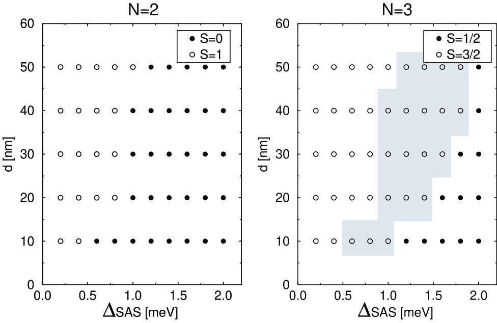
FIG. 3.: The ground-state spin of the double dot for $N=2$(left) or $N=3$(right) for $B=5$ T for a parabolic confinement potential $\hbar\omega_{0}=6.0$ meV. Shaded region corresponds to a transition from $S=0\rightarrow 3/2$

We now focus on a typical point in the shaded region, $d=16.0$ nm and $\Delta_{\rm SAS}=1.2$ meV. In Fig. 4 the total energy, total angular momentum and the total spin of the ground state for $N=2,3$ are plotted.

The difference between the total spin of two and three electrons systems is shown in the bottom panel of Fig. 5. The spin-blockade condition is satisfied for 4.0 $\leq B\leq 9.3$T, which is wider than for the single dot. In the bulk bilayer fractional quantum Hall (QH) systems, a phase diagram on the $\Delta_{\rm SAS}-d$ plane has been considered. If we translate[7] the quantities for the dots, we are working in the ‘two-component’ (correlation-dominated) region around the QH-non QH boundary in the language for the bilayer QH system. This might have some relevance to the behavior of the double dots. In Fig. 5, the excitation energies for the $S=1/2,3/2$ states are also plotted. The excitation energies for both $N=2$ and $N=3$ systems are about 0.12 meV (exceed 0.1 meV) at $B=6.4$ T, which is large enough for the spin blockade to be observed. We also notice a level crossing between the second and the third excited states around $B=6.9$ T for $N=3$, which should appear in the Coulomb diamond.

FIG. 4.: The total angular momentum and total spin of the ground state for double dots with $N=2$(left) $N=3$(right) electrons. $\hbar\omega_{0}=6.0$ meV. $d=16.0$ nm, and $\Delta_{\rm SAS}=1.2$ meV.

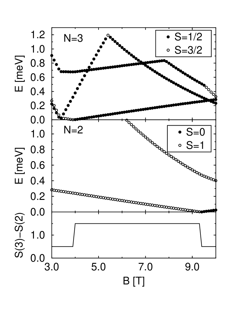
FIG. 5.: Top (middle): Excitation energies for $N=3$
$(N=2)$ double dots. Bottom: The difference, $S(3)-S(2)$, in the total spin for $N=2$ and $N=3$ double dots.

In summary, we have shown that in both single and double dots, a spin blockade should occur in some magnetic field region, as an effect of the total spin dominated by the magic angular momenta. We would like to thank to Seigo Tarucha and Guy Austing for a number of valuable discussions.

REFERENCES

- [1] D. Weinmann, W. Hausler, and B. Kramer, Phys. Rev. Lett. 74, 984 (1995): D. Weinmann et al., Europhys. Lett. 26, 467 (1994).
- [2] Y. Tanaka and H. Akera, Phys. Rev. B 44, 3901 (1996).
- [3] M. Eto, Jpn. J. Appl Phys. 36, 3924 (1997).
- [4] S. M. Girvin and T. Jach, Phys. Rev. B 28 (1983) 4506.
- [5] P.A. Maksym and T. Chakraborty, Phys. Rev. Lett. 65, 108 (1990).
- [6] P.A. Maksym, Phys. Rev. B 53, 10871 (1996).
- [7] H. Aoki, to appear in Physica E.
- [8] R. J. Galejs, Phys. Rev. B 35, 6240 (1987).
- [9] P. A. Maksym, L. D. Hallam and J. Weis, Physica B 212, 213 (1995).
- [10] H. Imamura, P.A. Maksym, and H. Aoki, to appear in Physica B.
- [11] P.A. Maksym nad T. Chakraborty, Phys. Rev. B 45, 1947 (1992).
- [12] V. Fock, Z. Phys. 47, 466 (1928); C.G. Darwin, Proc. Cambridge Philos. Soc. 27, 86 (1930).
- [13] S. Tarucha, D. G. Austing, and T. Honda, Phys. Rev. Lett. 77 3613 (1996).
- [14] P. A. Maksym and N. A. Bruce, to appear in Physica E.
- [15] D. G. Austing, T. Honda and S. Tarucha, Jpn. J. Appl. Phys. 36,11667 (1997).
- [16] H. Imamura, P.A. Maksym, and H. Aoki, Phys. Rev. B 52, 12613 (1996).
- [17] P.A. Maksym, H. Imamura, and H. Aoki, in Proc. 23rd Int. Conf. on the physics of Semiconductors (World Scientific, 1996) p.1613.
- [18] J. H. Oh et al., Phys. Rev. B 53, R13264 (1996).
- [19] J. J. Palacios and P. Hawrylak, Phys. Rev. B 51, 1769 (1995).
- [20] J. Hu, E. Dagotto, and A. H. MacDonald, Phys. Rev. B 54, 8616 (1996).
- [21] Hiroyuki Tamura, to appear in Physica B.