Dynamics of spin ladders

Abstract

We derive an approximate theory for Heisenberg spin ladders with two legs by mapping the spin dynamics onto the problem of hard-core ‘bond-Bosons’. The parameters of the Bosonic Hamiltonian are obtained by matching anomalous Green’s functions to Lanczos results and we find evidence for a strong renormalization due to quantum fluctuations. Various dynamical spin correlation functions are calculated and found to be in good agreement with Lanczos results. We then enlarge the effective Hamiltonian to describe the coupling of the Bosonic spin fluctuations to a single hole injected into the system and treat the hole-dynamics within the ‘rainbow-diagram’ approximation by Schmidt-Rink et. al. Theoretical predictions for the single hole spectral function are obtained and found to be in good agreement with Lanczos results.

I Introduction

Copper-oxides with a $CuO_{2}$ plane containing line-defects, which results in ladder-like arrangments of $Cu$-atoms[1], have recently received considerable attention[2]. In addition to being interesting physical systems themselves[3, 4], they may be considered, on the theoretical side, as an important stepping-stone to understand the fully $2D$ $CuO_{2}$ planes of cuprate superconductors. Namely their special geometry makes two-legged ladders a realization of a particularly simple ‘RVB’-type state, and developing a ‘technology’ for handling such RVB states clearly is one of the key issues in the theory of high-temperature superconductors. In the following, we want to derive a simple theoretical description of the spin dynamics and single-hole dynamics of ladders. Thereby we follow an approach which is similar in spirit to the Landau theory of Fermi liquids: we use a simple picture of an ‘RVB spin liquid’ and its excitation spectrum and parameterize the dispersion of the spin excitations by few parameters, which are then obtained by matching the results to Lanczos calculations and finite-size analysis. Using this parameterization we make quantitative predictions for various dynamical correlation functions which can be compared to exact diagonalization (and experiment). The theory actually allows to make rather detailed predictions, which in all cases studied are in good agreement with Lanczos results. We also discuss possibilities to extend the calculation to $2D$ systems.
We consider the standard $t-J$ model on a $2$-leg ladder with $N$ rungs. More precisely, the Hamiltonian reads

$$H=-\sum_{\langle i,j\rangle}(t_{ij}\;\hat{c}_{i,\sigma}^{\dagger}\hat{c}_{j,\sigma}+H.c.)+\sum_{\langle i,j\rangle}J_{ij}\;\mathchoice{{\hbox{\boldmath$\displaystyle S$}}}{{\hbox{\boldmath$\textstyle S$}}}{{\hbox{\boldmath$\scriptstyle S$}}}{{\hbox{\boldmath$\scriptscriptstyle S$}}}_{i}\cdot\mathchoice{{\hbox{\boldmath$\displaystyle S$}}}{{\hbox{\boldmath$\textstyle S$}}}{{\hbox{\boldmath$\scriptstyle S$}}}{{\hbox{\boldmath$\scriptscriptstyle S$}}}_{j}.$$ (1)

Here $\langle i,j\rangle$ denotes a summation over all pairs of nearest neighbors on the ladder, for bonds along the legs we choose $t_{ij}=t$ and $J_{ij}=J$, for bonds along the rungs $t_{ij}=t_{\perp}$ and $J_{ij}=J_{\perp}$. In the following we adopt the values $J_{\perp}=J$, $t_{\perp}=t$, and $J/t=0.5$, which may be roughly appropriate for actual the materials. We choose the $x$-axis along the direction of the legs, the $y$-axis along the rungs.

II Spin dynamics

To begin with, we consider the case of half-filling and, following Ref.[5] define the following operators:

$$s_{ij}^{\dagger} = \frac{1}{\sqrt{2}}(\hat{c}_{i,\uparrow}^{\dagger}\hat{c}_{j,\downarrow}^{\dagger}-\hat{c}_{i,\downarrow}^{\dagger}\hat{c}_{j,\uparrow}^{\dagger}),$$ (2)

$$t_{ij,x}^{\dagger} = \frac{-1}{\sqrt{2}}(\hat{c}_{i,\uparrow}^{\dagger}\hat{c}_{j,\uparrow}^{\dagger}-\hat{c}_{i,\downarrow}^{\dagger}\hat{c}_{j,\downarrow}^{\dagger})$$ (3)

$$t_{ij,y}^{\dagger} = \frac{i}{\sqrt{2}}(\hat{c}_{i,\uparrow}^{\dagger}\hat{c}_{j,\uparrow}^{\dagger}+\hat{c}_{i,\downarrow}^{\dagger}\hat{c}_{j,\downarrow}^{\dagger}),$$ (4)

$$t_{ij,z}^{\dagger} = \frac{1}{\sqrt{2}}(\hat{c}_{i,\uparrow}^{\dagger}\hat{c}_{j,\downarrow}^{\dagger}+\hat{c}_{i,\downarrow}^{\dagger}\hat{c}_{j,\uparrow}^{\dagger}).$$ (5)

These create either a singlet or the three components of a triplet on the sites $i$ and $j$. Following a large number of workers[5, 6, 7, 8], we will start out from the ‘rung-RVB state’, $|\Psi_{0}\rangle=\prod_{n=0}^{N}s_{n,n+\hat{y}}^{\dagger}|0\rangle$, which is the ground state in the limit $J_{\perp}/J\rightarrow\infty$ (here $i+\hat{y}$ denotes the nearest neighbor of $i$ in $y$-direction). Let us now consider the effect of switching on $J$. Obviously this will create ‘fluctuations’ in the vacuum state, and it is of importance to clarify the nature of these. Due to the product nature of the vacuum it is sufficient to consider just one $4$-site plaquette, see Figure 1 for the labelling of sites. For $J$$=$$0$ the ground state is $|0\rangle=s_{14}^{\dagger}s_{23}^{\dagger}|vac\rangle$, with energy $-(3/2)J_{\perp}$. It might appear that the fluctuation with the lowest cost in energy would be a ‘$90$-degree swap’, i.e. a transition to a state with singlets along the legs: $|1\rangle$$=$$s_{12}^{\dagger}s_{43}^{\dagger}|vac\rangle$. This state has energy $-(3/2)J$, i.e. it is degenerate with the vacuum in the limit $J_{\perp}$$=$$J$. This line of thinking, however, is incorrect. The reason is that $|1\rangle$ is not orthogonal to the vacuum, more precisely one finds $\langle 1|0\rangle=1/2$. The most natural way to proceed is to form the orthogonal complement $|2\rangle=|1\rangle-(1/2)|0\rangle$, which (after normalization) is found to be

$\displaystyle|2\rangle=\frac{1}{\sqrt{3}}(t_{14,x}^{\dagger}t_{23,x}^{\dagger}+t_{14,y}^{\dagger}t_{23,y}^{\dagger}+t_{14,z}^{\dagger}t_{23,z}^{\dagger})|vac\rangle.$

The (manifestly rotation invariant) expression on the r.h.s. thereby is nothing but the Clebsch-Gordan combination of two triplets along the rungs into a singlet.

FIG. 1.: Labelling of the sites in the $2\times 2$ plaquette.

This shows, that the ‘true’ excitation is the double triplet, rather than a state with singlets along the legs, or, put another way, that the state $|1\rangle$ is redundant and can be discarded if we keep $|0\rangle$ and $|2\rangle$. The same holds true for the last candidate state for a fluctuation, namely two triplets along the legs coupled to a singlet:

$\displaystyle|3\rangle=\frac{1}{\sqrt{3}}(t_{12,x}^{\dagger}t_{43,x}^{\dagger}+t_{12,y}^{\dagger}t_{43,y}^{\dagger}+t_{12,z}^{\dagger}t_{43,z}^{\dagger})|vac\rangle.$

Again we find that this state is not orthogonal to the vacuum either, and orthogonalization again yields $|2\rangle$. The only fluctuation we have to take into account therefore is the formation of two triplets on adjacent rungs, the respective matrix element is $\langle t_{14,z}t_{23,z}|H|s_{14}^{\dagger}s_{23}^{\dagger}\rangle=J/2$. The energy increases by $2J_{\perp}$, which we interpret as twice the ‘energy of formation’ of a single triplet. Let us now assume that a double triplet has been formed, and consider its further development. First, the two triplets can ‘recombine’ and we return to the vacuum; the matrix element for this process again is $J/2$. Second, the two triplets can ‘swap their species’. More precisely, for $\alpha$$\neq$$\beta$ there is a matrix element of the form $\langle t_{14,\beta}t_{23,\beta}|H|t_{14,\alpha}^{\dagger}t_{23,\alpha}^{\dagger}\rangle$$=$$-J/2$. The last possibility is that one of the triplets interacts with a singlet on the as yet ‘untouched’ rung next to it. To study this in more detail we consider a $4$-site plaquette containing spin $1$. It is convenient to form the states

$\displaystyle|\pm\rangle=\frac{1}{\sqrt{2}}(t_{14,z}^{\dagger}s_{23}^{\dagger}\pm s_{14}^{\dagger}t_{23,z}^{\dagger})|vac\rangle$

which do have definite parities under the mirror operations $\sigma_{x}$ and $\sigma_{y}$ (see Figure 1). They are triplets with $z$-component $0$. Next we consider which state could mix with one of these states. A first possibility would be two ‘rung triplets’, coupled to a triplet:

$\displaystyle|4\rangle=\frac{1}{\sqrt{2}}(t_{14,x}^{\dagger}t_{23,y}^{\dagger}-t_{14,y}^{\dagger}t_{23,x}^{\dagger})|vac\rangle.$

However, this state has positive parity under $x$-reflection, whereas $|\pm\rangle$ both have negative parity. This state therefore cannot be admixed[5]. The next possibility is

$\displaystyle|5\rangle=\frac{1}{\sqrt{2}}(t_{12,z}^{\dagger}s_{43}^{\dagger}-s_{12}^{\dagger}t_{43,z}^{\dagger})|vac\rangle,$

(which does have the required negative $x$-parity), but this state is actually identical to $|-\rangle$. Finally, one could think of two triplets along the legs coupled to form a triplet:

$\displaystyle|6\rangle=\frac{1}{\sqrt{2}}(t_{12,x}^{\dagger}t_{43,y}^{\dagger}-t_{12,y}^{\dagger}t_{43,x}^{\dagger})|vac\rangle.$

but, in fact, $|6\rangle=|+\rangle$. The only process possible for the rung-triplet therefore is to ‘propagate’, i.e. exchange its position with a singlet on a neighboring rung. The hopping element is $(\langle+|H|+\rangle-\langle-|H-\rangle)/2=J/2$. The ‘90-degree swap’ to a triplet along the leg (see the state $|5\rangle$) would give a redundant state and, most importantly, ‘anharmonic processes’ whereby a triplet decays into two triplets (see the states $|5\rangle$ or $|6\rangle$) are not possible either. Clearly, this absence of anharmonicity leads to a considerable simplification of the physics - it is the ultimate reason why, as will be seen later, the spin correlation function in a ladder is remarkably ‘coherent’.
There is one last process we need to discuss. It may happen that two triplets of unlike species which have been created in different pair creation processes ‘collide’. More precisely, for $\alpha\neq\beta$ there is a matrix element of the type $\langle t_{14,\beta}t_{23,\alpha}|H|t_{14,\alpha}^{\dagger}t_{23,\beta}^{\dagger}\rangle$$=$$J/2$, which describes two triplets of unlike species ‘hopping over’ one another.
We now represent the presence of a triplet on the $n^{th}$ rung by the presence of a ‘book-keeping boson’ created by $t_{n,\alpha}^{\dagger}$. Grouping the three possible triplet states into a single 3-vector, $\mathchoice{{\hbox{\boldmath$\displaystyle t$}}}{{\hbox{\boldmath$\textstyle t$}}}{{\hbox{\boldmath$\scriptstyle t$}}}{{\hbox{\boldmath$\scriptscriptstyle t$}}}_{n}$$=$$(t_{n,x},t_{n,y},t_{n,z})$, we can describe all processes involving non-redundant states by the following manifestly rotation-invariant Hamiltonian

$$H = J_{\perp}\sum_{n}\mathchoice{{\hbox{\boldmath$\displaystyle t$}}}{{\hbox{\boldmath$\textstyle t$}}}{{\hbox{\boldmath$\scriptstyle t$}}}{{\hbox{\boldmath$\scriptscriptstyle t$}}}_{n}^{\dagger}\cdot\mathchoice{{\hbox{\boldmath$\displaystyle t$}}}{{\hbox{\boldmath$\textstyle t$}}}{{\hbox{\boldmath$\scriptstyle t$}}}{{\hbox{\boldmath$\scriptscriptstyle t$}}}_{n}$$ (6)

$$+ \frac{J}{2}\sum_{n}(\;\mathchoice{{\hbox{\boldmath$\displaystyle t$}}}{{\hbox{\boldmath$\textstyle t$}}}{{\hbox{\boldmath$\scriptstyle t$}}}{{\hbox{\boldmath$\scriptscriptstyle t$}}}_{n}^{\dagger}\cdot\mathchoice{{\hbox{\boldmath$\displaystyle t$}}}{{\hbox{\boldmath$\textstyle t$}}}{{\hbox{\boldmath$\scriptstyle t$}}}{{\hbox{\boldmath$\scriptscriptstyle t$}}}_{n+1}^{\dagger}+H.c.\;)+\frac{J}{2}\sum_{n}(\;\mathchoice{{\hbox{\boldmath$\displaystyle t$}}}{{\hbox{\boldmath$\textstyle t$}}}{{\hbox{\boldmath$\scriptstyle t$}}}{{\hbox{\boldmath$\scriptscriptstyle t$}}}_{n}^{\dagger}\cdot\mathchoice{{\hbox{\boldmath$\displaystyle t$}}}{{\hbox{\boldmath$\textstyle t$}}}{{\hbox{\boldmath$\scriptstyle t$}}}{{\hbox{\boldmath$\scriptscriptstyle t$}}}_{n+1}+H.c.\;)$$ (7)

$$- \frac{J}{2}\sum_{n}(\;\mathchoice{{\hbox{\boldmath$\displaystyle t$}}}{{\hbox{\boldmath$\textstyle t$}}}{{\hbox{\boldmath$\scriptstyle t$}}}{{\hbox{\boldmath$\scriptscriptstyle t$}}}_{n}^{\dagger}\cdot\mathchoice{{\hbox{\boldmath$\displaystyle t$}}}{{\hbox{\boldmath$\textstyle t$}}}{{\hbox{\boldmath$\scriptstyle t$}}}{{\hbox{\boldmath$\scriptscriptstyle t$}}}_{n+1}^{\dagger}\;\mathchoice{{\hbox{\boldmath$\displaystyle t$}}}{{\hbox{\boldmath$\textstyle t$}}}{{\hbox{\boldmath$\scriptstyle t$}}}{{\hbox{\boldmath$\scriptscriptstyle t$}}}_{n+1}\cdot\mathchoice{{\hbox{\boldmath$\displaystyle t$}}}{{\hbox{\boldmath$\textstyle t$}}}{{\hbox{\boldmath$\scriptstyle t$}}}{{\hbox{\boldmath$\scriptscriptstyle t$}}}_{n}-\mathchoice{{\hbox{\boldmath$\displaystyle t$}}}{{\hbox{\boldmath$\textstyle t$}}}{{\hbox{\boldmath$\scriptstyle t$}}}{{\hbox{\boldmath$\scriptscriptstyle t$}}}_{n}^{\dagger}\cdot\mathchoice{{\hbox{\boldmath$\displaystyle t$}}}{{\hbox{\boldmath$\textstyle t$}}}{{\hbox{\boldmath$\scriptstyle t$}}}{{\hbox{\boldmath$\scriptscriptstyle t$}}}_{n+1}\;\mathchoice{{\hbox{\boldmath$\displaystyle t$}}}{{\hbox{\boldmath$\textstyle t$}}}{{\hbox{\boldmath$\scriptstyle t$}}}{{\hbox{\boldmath$\scriptscriptstyle t$}}}_{n+1}^{\dagger}\cdot\mathchoice{{\hbox{\boldmath$\displaystyle t$}}}{{\hbox{\boldmath$\textstyle t$}}}{{\hbox{\boldmath$\scriptstyle t$}}}{{\hbox{\boldmath$\scriptscriptstyle t$}}}_{n}\;).$$ (8)

This Hamiltonian has also been derived by Gopalan et al.[5]. The form of the Hamiltonian (8) suggests a quite obvious approximation, namely to break down the quartic terms in a BCS-like fashion, e.g.:

$$t_{n,\beta}^{\dagger}t_{n+1,\beta}^{\dagger}t_{n+1,\alpha}t_{n,\alpha} \rightarrow \Delta\;t_{n,\beta}^{\dagger}t_{n+1,\beta}^{\dagger}+\Delta^{*}\;t_{n+1,\alpha}t_{n,\alpha}$$ (9)

$$\Delta = \langle t_{n+1,\alpha}t_{n,\alpha}\rangle.$$ (10)

As a next step, we might assume that the hopping integrals and pair creation matrix elements in (8) are renormalized in a Gutzwiller-like fashion, to mimic the effect of the hard-core constraint. After Fourier transform, we would thus arrive at an approximate Hamiltonian of the form

$$H_{eff} = \sum_{k>0}\;[\;(\tilde{\epsilon}_{k}\;\mathchoice{{\hbox{\boldmath$\displaystyle t$}}}{{\hbox{\boldmath$\textstyle t$}}}{{\hbox{\boldmath$\scriptstyle t$}}}{{\hbox{\boldmath$\scriptscriptstyle t$}}}_{k}^{\dagger}\cdot\mathchoice{{\hbox{\boldmath$\displaystyle t$}}}{{\hbox{\boldmath$\textstyle t$}}}{{\hbox{\boldmath$\scriptstyle t$}}}{{\hbox{\boldmath$\scriptscriptstyle t$}}}_{k}+\tilde{\epsilon}_{-k}\;\mathchoice{{\hbox{\boldmath$\displaystyle t$}}}{{\hbox{\boldmath$\textstyle t$}}}{{\hbox{\boldmath$\scriptstyle t$}}}{{\hbox{\boldmath$\scriptscriptstyle t$}}}_{-k}^{\dagger}\cdot\mathchoice{{\hbox{\boldmath$\displaystyle t$}}}{{\hbox{\boldmath$\textstyle t$}}}{{\hbox{\boldmath$\scriptstyle t$}}}{{\hbox{\boldmath$\scriptscriptstyle t$}}}_{-k})$$ (11)

$$\;\;\;\;\;\;\;\;+(\tilde{\Delta}_{k}\;\mathchoice{{\hbox{\boldmath$\displaystyle t$}}}{{\hbox{\boldmath$\textstyle t$}}}{{\hbox{\boldmath$\scriptstyle t$}}}{{\hbox{\boldmath$\scriptscriptstyle t$}}}_{k}^{\dagger}\cdot\mathchoice{{\hbox{\boldmath$\displaystyle t$}}}{{\hbox{\boldmath$\textstyle t$}}}{{\hbox{\boldmath$\scriptstyle t$}}}{{\hbox{\boldmath$\scriptscriptstyle t$}}}_{-k}^{\dagger}+H.c.)\;].$$ (12)

Assuming that the $t$ in this Hamiltonian are free Bosons this is readily solved by the ansatz

$$\mathchoice{{\hbox{\boldmath$\displaystyle\gamma$}}}{{\hbox{\boldmath$\textstyle\gamma$}}}{{\hbox{\boldmath$\scriptstyle\gamma$}}}{{\hbox{\boldmath$\scriptscriptstyle\gamma$}}}_{k,\alpha} = u_{k}\mathchoice{{\hbox{\boldmath$\displaystyle t$}}}{{\hbox{\boldmath$\textstyle t$}}}{{\hbox{\boldmath$\scriptstyle t$}}}{{\hbox{\boldmath$\scriptscriptstyle t$}}}_{k}+v_{k}\mathchoice{{\hbox{\boldmath$\displaystyle t$}}}{{\hbox{\boldmath$\textstyle t$}}}{{\hbox{\boldmath$\scriptstyle t$}}}{{\hbox{\boldmath$\scriptscriptstyle t$}}}_{-k}^{\dagger}$$ (13)

$$\mathchoice{{\hbox{\boldmath$\displaystyle\gamma$}}}{{\hbox{\boldmath$\textstyle\gamma$}}}{{\hbox{\boldmath$\scriptstyle\gamma$}}}{{\hbox{\boldmath$\scriptscriptstyle\gamma$}}}_{-k,\alpha}^{\dagger} = v_{k}\mathchoice{{\hbox{\boldmath$\displaystyle t$}}}{{\hbox{\boldmath$\textstyle t$}}}{{\hbox{\boldmath$\scriptstyle t$}}}{{\hbox{\boldmath$\scriptscriptstyle t$}}}_{k}+u_{k}\mathchoice{{\hbox{\boldmath$\displaystyle t$}}}{{\hbox{\boldmath$\textstyle t$}}}{{\hbox{\boldmath$\scriptstyle t$}}}{{\hbox{\boldmath$\scriptscriptstyle t$}}}_{-k}^{\dagger},$$ (14)

to give the ($3$-fold degenerate) dispersion

$$\omega_{k}=\sqrt{\tilde{\epsilon}_{k}^{2}-\tilde{\Delta}_{k}^{2}}.$$ (15)

The parameters $\tilde{\epsilon}_{k}$, $\tilde{\Delta}_{k}$ should be calculated in some approximate fashion, by mean-field and Gutzwiller-approximation to the original Hamiltonian (8)[5]. We note, however, that there are a number of difficulties with such an approach: the density of Bosons $n_{b}$ can be obtained from the spin correlation function along the rungs using the identity $-3(1-n_{b})/4+n_{b}/4=\langle\mathchoice{{\hbox{\boldmath$\displaystyle S$}}}{{\hbox{\boldmath$\textstyle S$}}}{{\hbox{\boldmath$\scriptstyle S$}}}{{\hbox{\boldmath$\scriptscriptstyle S$}}}_{i}\cdot\mathchoice{{\hbox{\boldmath$\displaystyle S$}}}{{\hbox{\boldmath$\textstyle S$}}}{{\hbox{\boldmath$\scriptstyle S$}}}{{\hbox{\boldmath$\scriptscriptstyle S$}}}_{i+\hat{y}}\rangle$. The spin correlation function thereby can be estimated from exact diagonalization results. For $J_{\perp}/J=1$ we thus obtain $n_{b}\approx 0.3$. The quantum fluctuations thus are strong, and we may expect that the matrix elements for propagation and pair creation in (8) are heavily renormalized. On the other hand, the matrix elements of the quartic terms in (8) will not be renormalized at all due to the hard-core constraint, because these terms do not change the Boson occupation of any site. We may thus expect a subtle interplay of Gutzwiller projection and mean-field decomposition and to avoid poorly controlled approximations we resort to numerical techniques to extract the parameters of the Hamiltonian (12) and, in doing so, moreover check the quality of the mapping to noninteracting Bosons per se. To that end we define the operator

$\displaystyle\tau_{n}^{\dagger}=\frac{1}{2}(n_{n,\uparrow}n_{n+\hat{y},\downarrow}-n_{n,\downarrow}n_{n+\hat{y},\uparrow}-S_{n}^{+}S_{n+\hat{y}}^{-}+S_{n}^{-}S_{n+\hat{y}}^{+}).$

If the rung $(n,n+\hat{y})$ is in a singlet state, $\tau_{n}^{\dagger}$ transforms it into the $z$-component of the triplet; if the rung is in any of the triplet states, the state is annihilated. This operator, while acting entirely within the Hilbert space of the original ladder system, thus may be viewed as a realization of the hard-core Boson creation operator. Next, using standard Lanczos techniques, we evaluate the following Green’s functions:

$$A_{+}(k,\omega) = \Im\frac{1}{\pi}\langle\Psi_{0}|\tau_{-k}\frac{1}{\omega-(H-E_{0})-i0^{+}}\tau_{-k}^{\dagger}|\Psi_{0}\rangle,$$ (16)

$$A_{-}(k,\omega) = \Im\frac{1}{\pi}\langle\Psi_{0}|\tau_{k}^{\dagger}\frac{1}{\omega-(H-E_{0})-i0^{+}}\tau_{k}|\Psi_{0}\rangle,$$ (17)

$$A_{int}(k,\omega) = \Im\frac{1}{\pi}\langle\Psi_{0}|\tau_{k}^{\dagger}\frac{1}{\omega-(H-E_{0})-i0^{+}}\tau_{-k}^{\dagger}|\Psi_{0}\rangle,$$ (18)

where $|\Psi_{0}\rangle$ ($E_{0}$) denote the ground state wave function (energy) of the ladder and $\tau_{k}^{\dagger}$ is the (1 dimensional) Fourier transform of $\tau_{n}^{\dagger}$. Our goal is to map the spin excitations of the ladder onto a system of free ‘Quasi-Bosons’ goverened by the Hamiltonian (12). If we want to compare spectral properties, we have to take into account that the spectral weight of the hard-core Bosons may be strongly renormalized. For example, as a rigorous identity we have $\langle[\tau_{i},\tau_{i}^{\dagger}]\rangle$$=$$1-4n_{b}/3$$\approx$$0.6$, rather than $1$ as it would be for free Bosons. To discuss the spectral functions we therefore assume that $\tau_{k}$$\rightarrow$$\sqrt{Z}t_{k}$, where $t_{k}$ is a free Boson operator, and $Z$ the wave function renormalization constant.
Assuming then that the free Bosons $t_{k}$ are indeed described by a Hamiltonian of the form (12) one can derive the following expressions for the above Green’s functions:

$$\omega A_{int}(k,\omega) = -\frac{Z\tilde{\Delta}_{k}}{2}\delta(\omega-\omega_{k})$$ (19)

$$\omega(A_{+}(k,\omega)+A_{-}(k,\omega)) = Z\tilde{\epsilon}_{k}\delta(\omega-\omega_{k}).$$ (20)

$$A_{+}(k,\omega)-A_{-}(k,\omega) = Z\delta(\omega-\omega_{k}).$$ (21)

In other words, the wave function renormalization $Z$ as well as the energy $\tilde{\epsilon}_{k}$ and pair creation amplitude $\tilde{\Delta}_{k}$ can be read off from the dispersion of the pole strength in the Green’s functions (21). Then, using the obtained values of $\tilde{\epsilon}_{k}$ and $\tilde{\Delta}_{k}$ to calculate the dispersion of the excitation energy from (15) and comparing with the actual numerical values should provide a stringent cross-check for the validity of the mapping to the free-Boson Hamiltonian (12). Figure 2 compares $A_{+}(k,\omega)$ and $\omega A_{int}(k,\omega)$ and $\omega(A_{+}(k,\omega)+A_{-}(k,\omega))$. To begin with, the $A_{+}(k,\omega)$ shows a series of sharp dispersive peaks, which however trace out a rather unusual dispersion with a shallow local minimum at $k$$=$$0$. Next, $\omega A_{int}(k,\omega)$ has a pronounced low energy peak too, which coincides with that of $A_{+}(k,\omega)$. The residuum changes sign at approximately $k=\pi/2$ (note that $A_{int}$ is an off-diagonal matrix element of the resolvent operator; its residuum therefore need not be positive definite), the magnitude is nearly identical at $k$$=$$0$ and $k$$=$$\pi$. This suggests a $k$-dependence of the form $\tilde{\Delta}_{k}\propto\cos(k)$, as one would expect for a pair amplitude corresponding to pair creation on nearest neighbors. Similarly, $\omega(A_{+}(k,\omega)+A_{-}(k,\omega))$ shows low energy peaks coniciding with those of $A_{+}(k,\omega)$. The dispersion of the weight, however, is more complicated than for the pairing amplitude.

FIG. 2.: Spectral functions $A_{+}(k,\omega)$ (full line), $\omega(A_{+}(k,\omega)+A_{-}(k,\omega))$ (dashed line) and $\omega A_{int}(k,\omega)$ (dotted line) obtained by Lanczos diagonalization of a $2\times 10$ ladder. $\delta$-functions are replaced by Lorentzians of width $0.1J$.

For a quantitative analysis, we proceed to Figure 3. Part (a) shows first of all the weight $Z$ obtained from $A_{+}(k,\omega)-A_{-}(k,\omega)$. Remarkably enough, $Z$ is quite independent of $k$ and moreover close to the estimate of $0.6$ obtained from $\langle[\tau_{i},\tau_{i}^{\dagger}]\rangle$. The fact that $Z$ is indeed fairly $k$-independent is a first indication for the applicability of a free Boson Hamiltonian. To avoid a proliferation of adjustable parameters we take the $k$-average, which is $Z$$=$$0.53$ (nearly independent of $N$ for $N>6$). Using this value of $Z$ we then calculated the $\tilde{\epsilon}_{k}$ and $\tilde{\Delta}_{k}$ and Fourier transform them with respect to $k$. For simplicity, we terminate the Fourier series after the third (i.e. $\cos(2k)$-like) term. This gives already a very satisfactory fit to the data, as seen in Figure 3. Figure 3b shows the comparison of the numerical excitation energy and the dispersion calculated from (15), using the values of $\tilde{\epsilon}_{k}$ and $\tilde{\Delta}_{k}$ extracted from the weights of the correlation functions. There is quite reasonable agreement, which indicates that the effective free-Boson Hamiltonian itself is a quite good description of the spin dynamics.
We proceed to extrapolate the results to the infinite chain. To that end, we performed the calculation for different $N$ and calculated the Fourier coefficients of $\tilde{\epsilon}_{k}$ and $\tilde{\Delta}_{k}$. Then, Figures 3(c) and (d) show plots of these Fourier coefficients vs. $1/N^{2}$. The plots rather obviously suggest that all of the Fourier coefficients can be

FIG. 3.: (a): $\tilde{\epsilon}_{k}$ (triangles), $\tilde{\Delta}_{k}$ (squares), and $Z$ (hexagons) as obtained from the pole-strengths of the Greens functions plotted versus momentum. The continuous line gives Fourier expansions with the lowest $3$ harmonics.
(b): $\omega_{k}$ calculated from (15) (triangles) compared to the exact excitation energies (squares).
(c) and (d): Scaling of the Fourier coefficients of $\Delta$ and $\epsilon$ with the length of the ladder.

expressed as $c(N)=c_{\infty}+c^{\prime}/N^{2}$ to good accuracy. The extrapolated values $c_{\infty}$ are given in Table I. We note in passing that these values give a ‘spin gap’ (i.e. the energy of the triplet with $k=\pi$) of $0.51J$, in agreement with exact diagonalization[9] and DMRG calculations[10]. Let us now briefly discuss these values. For the pairing amplitude $\tilde{\Delta}_{k}$ we have a by far dominant $\cos(k)$-component, $\Delta_{1}$, consistent with pair creation/annihilation on nearest neighbors. The second-nearest neighbor amplitude is substantially smaller, and also the uniform component is very small.
The results for the renormalized energy $\tilde{\epsilon}_{k}$ are more surprising. To begin with, the constant term is $1.77J$, rather than $J_{\perp}$$=$$J$, as one would expect. A possible explanation for this strong increase is that a triplet on (say) the rung number $i$ blocks the ‘pair creation’ of triplets on the pairs $(i-1,i)$ and $(i,i+1)$. The corresponding loss of fluctuation energy increases the energy cost for creating a triplet, i.e. the on-site energy of a triplet. In addition, presence of a triplet will partially inhibit the motion of other triplets and thus cause a further loss of delocalization energy. Quite obviously these effects combined are quite substantial. Next, the coefficient of the nearest-neighbor harmonic is rather small (only $0.21$). This may be understood simply in terms of a Gutzwiller-like reduction of the mobility due to the ‘excluded volume’ occupied by other triplets. Moreover, the terms which describe the ‘exchange hopping’ and effectively propagate a triplet by one lattice site may interfere destructively with the ‘ordinary’ motion of a triplet, and thus reduce the effective hopping integral. A further surprise is the large amplitude for second-nearest neighbor hopping. Here one could envisage processes where the propagating triplet encounters a pair of triplets, recombines with one of them and thereby transfers its momentum to the remaining triplet, so that the propagating triplet effectively has been transferred by two sites. Such a process would be proportional to the probability of finding a quantum fluctuation, which is rather high in the present case. All in all, the data show that the propagation of the triplets is strongly renormalized in the relatively dense and strongly interacting ‘background’ of the other triplets.
Assuming that the ‘effective Hamiltonian’ (12) with the extrapolated parameters in Table I gives a good description of the spin dynamics, we proceed to calculate dynamical correlation functions relevant to experiment. We consider the spin operator on a single rung and ‘translate it’ into the language of the hard-core Bosons. The operator $S_{\alpha}(k_{\perp}$$=$$\pi)$ turns a singlet into an $\alpha$-triplet and vice versa; the other two types of triplets are annihilated, whence: $\mathchoice{{\hbox{\boldmath$\displaystyle S$}}}{{\hbox{\boldmath$\textstyle S$}}}{{\hbox{\boldmath$\scriptstyle S$}}}{{\hbox{\boldmath$\scriptscriptstyle S$}}}(k_{\perp}$$=$$\pi)\rightarrow\mathchoice{{\hbox{\boldmath$\displaystyle t$}}}{{\hbox{\boldmath$\textstyle t$}}}{{\hbox{\boldmath$\scriptstyle t$}}}{{\hbox{\boldmath$\scriptscriptstyle t$}}}^{\dagger}$$+$$\textstyle t$. Next, the operator $S_{z}(k_{\perp}$$=$$0)$ annihilates a singlet and converts e.g. $t_{x}^{\dagger}$$\rightarrow$$it_{y}^{\dagger}$ (compare (5)). $\mathchoice{{\hbox{\boldmath$\displaystyle S$}}}{{\hbox{\boldmath$\textstyle S$}}}{{\hbox{\boldmath$\scriptstyle S$}}}{{\hbox{\boldmath$\scriptscriptstyle S$}}}(k_{\perp}$$=$$0)$ therefore must be bilinear in the triplet operators and the only possibility is $\mathchoice{{\hbox{\boldmath$\displaystyle t$}}}{{\hbox{\boldmath$\textstyle t$}}}{{\hbox{\boldmath$\scriptstyle t$}}}{{\hbox{\boldmath$\scriptscriptstyle t$}}}^{\dagger}\times\mathchoice{{\hbox{\boldmath$\displaystyle t$}}}{{\hbox{\boldmath$\textstyle t$}}}{{\hbox{\boldmath$\scriptstyle t$}}}{{\hbox{\boldmath$\scriptscriptstyle t$}}}$. From its acting on $t_{x}^{\dagger}$ the prefactor must be $-i$, whence: $\mathchoice{{\hbox{\boldmath$\displaystyle S$}}}{{\hbox{\boldmath$\textstyle S$}}}{{\hbox{\boldmath$\scriptstyle S$}}}{{\hbox{\boldmath$\scriptscriptstyle S$}}}(k_{\perp}$$=$$0)$$\rightarrow$$-i\mathchoice{{\hbox{\boldmath$\displaystyle t$}}}{{\hbox{\boldmath$\textstyle t$}}}{{\hbox{\boldmath$\scriptstyle t$}}}{{\hbox{\boldmath$\scriptscriptstyle t$}}}^{\dagger}\times\mathchoice{{\hbox{\boldmath$\displaystyle t$}}}{{\hbox{\boldmath$\textstyle t$}}}{{\hbox{\boldmath$\scriptstyle t$}}}{{\hbox{\boldmath$\scriptscriptstyle t$}}}$. Obviously this is also the only way to construct a Hermitean operator ($\mathchoice{{\hbox{\boldmath$\displaystyle S$}}}{{\hbox{\boldmath$\textstyle S$}}}{{\hbox{\boldmath$\scriptstyle S$}}}{{\hbox{\boldmath$\scriptscriptstyle S$}}}(k_{\perp}$$=$$0)$ is the operator of total spin on one rung) from the triplets. A subtle point is the renormalization of the spectral weight: whereas $\mathchoice{{\hbox{\boldmath$\displaystyle S$}}}{{\hbox{\boldmath$\textstyle S$}}}{{\hbox{\boldmath$\scriptstyle S$}}}{{\hbox{\boldmath$\scriptscriptstyle S$}}}(k_{\perp}$$=$$\pi)$ actually changes the number of Quasi-Bosons and thus should be renormalized in a similar fashion as the hard-core Boson addition and removal spectra, $\mathchoice{{\hbox{\boldmath$\displaystyle S$}}}{{\hbox{\boldmath$\textstyle S$}}}{{\hbox{\boldmath$\scriptstyle S$}}}{{\hbox{\boldmath$\scriptscriptstyle S$}}}(k_{\perp}$$=$$0)$ does not change the Boson occupation of any rung and thus should remain essentially unrenormalized. Based on these considerations, we multiply $\mathchoice{{\hbox{\boldmath$\displaystyle S$}}}{{\hbox{\boldmath$\textstyle S$}}}{{\hbox{\boldmath$\scriptstyle S$}}}{{\hbox{\boldmath$\scriptscriptstyle S$}}}(k_{\perp}$$=$$\pi)$ by $\sqrt{Z}$, but leave $\mathchoice{{\hbox{\boldmath$\displaystyle S$}}}{{\hbox{\boldmath$\textstyle S$}}}{{\hbox{\boldmath$\scriptstyle S$}}}{{\hbox{\boldmath$\scriptscriptstyle S$}}}(k_{\perp}$$=$$0)$ unrenormalized. Then, upon Fourier transformation of the single rung operators and switching to the bond-Bosons we obtain the spin correlation functions:

$$S(q,\pi,z) = \frac{Z}{2}\frac{(u_{q}-v_{q})^{2}}{z-\omega_{k}},$$ (22)

$$S(q,0,z) = \frac{1}{2N}\sum_{k}\frac{(u_{k+q}v_{k}-u_{-k}v_{-(k+q)})^{2}}{z-(\omega_{k+q}+\omega_{k})}.$$ (23)

Note that $S(q,0,z)\rightarrow 0$ for $q\rightarrow 0$; this is what must come out because unlike conventional spin-wave theory the ‘rung-RVB’ state is an exact singlet, and both Hamiltonians, (8) and (12) are rotationally invariant; the ground state thus is an exact singlet, whence the operator of total spin must annihilate it. The obtained spin correlation functions are shown in Figure 4. We first note the rather different intensity of the two correlations functions. As

FIG. 4.: Spin correlation function $S(\mathchoice{{\hbox{\boldmath$\displaystyle q$}}}{{\hbox{\boldmath$\textstyle q$}}}{{\hbox{\boldmath$\scriptstyle q$}}}{{\hbox{\boldmath$\scriptscriptstyle q$}}},\omega-i\cdot 0.1J)$ obtained by numerical evaluation of (23 (full line) compared to the result of Lanczos diagonalization on an $N$$=$$12$ ladder (dotted line). Spectra for $q_{y}$$=$$0$ are multiplied by a factor of $5$.

could be expected on the basis of (23), the correlation function for $q_{y}$$=$$\pi$ consists essentially of a single peak, whereas the spectrum for $q_{y}$$=$$0$ has more ‘cusp-like’ appearance. It is interesting to note that these differences are reproduced quite well by the results of Lanczos calculation, which are also shown in Figure (4): the $q_{y}$$=$$\pi$ spectrum is indeed remarkably sharp, with nearly all the spectral weight concentrated in just one peak for every momentum. It should be noted that the agreement of the dispersion is not really surprising, this was actually seen already in Figure 3. The dispersion of the peak intensity, however, also agrees very well with the Lanczos result and thus provides further evidence for the correctness of the mapping to the Boson Hamiltonian.
By contrast, the spectra for $q_{y}=0$ usually consist of several peaks and one can already envisage how these spectra develop into the cusp-like spectra produced by our theory. The dispersion of the ‘peaks’ for $q_{y}$$=$$0$ is in good agreement with theory, showing a shallow maximum at $q_{x}$$\approx$$3\pi/5$ and approaching zero for $q_{x}\rightarrow 0$. All in all, the spin correlation function is obviously very well reproduced by our calculation. We proceed to a discussion of the ‘energy correlation function’ $e_{\alpha}(\mathchoice{{\hbox{\boldmath$\displaystyle q$}}}{{\hbox{\boldmath$\textstyle q$}}}{{\hbox{\boldmath$\scriptstyle q$}}}{{\hbox{\boldmath$\scriptscriptstyle q$}}},\omega)$, i.e. the dynamical correlation function of the operator

$\displaystyle H_{\alpha}(\mathchoice{{\hbox{\boldmath$\displaystyle q$}}}{{\hbox{\boldmath$\textstyle q$}}}{{\hbox{\boldmath$\scriptstyle q$}}}{{\hbox{\boldmath$\scriptscriptstyle q$}}})=\frac{1}{\sqrt{N}}\sum_{i}e^{i\mathchoice{{\hbox{\boldmath$\displaystyle q$}}}{{\hbox{\boldmath$\textstyle q$}}}{{\hbox{\boldmath$\scriptstyle q$}}}{{\hbox{\boldmath$\scriptscriptstyle q$}}}\cdot\mathchoice{{\hbox{\boldmath$\displaystyle R$}}}{{\hbox{\boldmath$\textstyle R$}}}{{\hbox{\boldmath$\scriptstyle R$}}}{{\hbox{\boldmath$\scriptscriptstyle R$}}}_{i}}\mathchoice{{\hbox{\boldmath$\displaystyle S$}}}{{\hbox{\boldmath$\textstyle S$}}}{{\hbox{\boldmath$\scriptstyle S$}}}{{\hbox{\boldmath$\scriptscriptstyle S$}}}_{i}\cdot\mathchoice{{\hbox{\boldmath$\displaystyle S$}}}{{\hbox{\boldmath$\textstyle S$}}}{{\hbox{\boldmath$\scriptstyle S$}}}{{\hbox{\boldmath$\scriptscriptstyle S$}}}_{i+\hat{\alpha}}.$

Apart from being a further probe of the spin dynamics, this correlation function plays a key role in the theory of phonon-assisted two-magnon absorption by Lorenzana and Sawatzky[11]. It therefore can be probed experimentally in infra-red absorption measurements. Here we restrict ourselves to the operator $H_{y}(\mathchoice{{\hbox{\boldmath$\displaystyle q$}}}{{\hbox{\boldmath$\textstyle q$}}}{{\hbox{\boldmath$\scriptstyle q$}}}{{\hbox{\boldmath$\scriptscriptstyle q$}}})$, which is easy to ‘translate’ to the Quasi-Boson system. Namely one can replace

$\displaystyle\mathchoice{{\hbox{\boldmath$\displaystyle S$}}}{{\hbox{\boldmath$\textstyle S$}}}{{\hbox{\boldmath$\scriptstyle S$}}}{{\hbox{\boldmath$\scriptscriptstyle S$}}}_{i}\cdot\mathchoice{{\hbox{\boldmath$\displaystyle S$}}}{{\hbox{\boldmath$\textstyle S$}}}{{\hbox{\boldmath$\scriptstyle S$}}}{{\hbox{\boldmath$\scriptscriptstyle S$}}}_{i+\hat{\alpha}}\rightarrow\mathchoice{{\hbox{\boldmath$\displaystyle t$}}}{{\hbox{\boldmath$\textstyle t$}}}{{\hbox{\boldmath$\scriptstyle t$}}}{{\hbox{\boldmath$\scriptscriptstyle t$}}}_{i}^{\dagger}\cdot\mathchoice{{\hbox{\boldmath$\displaystyle t$}}}{{\hbox{\boldmath$\textstyle t$}}}{{\hbox{\boldmath$\scriptstyle t$}}}{{\hbox{\boldmath$\scriptscriptstyle t$}}}_{i}$

whence

$\displaystyle e_{y}(\mathchoice{{\hbox{\boldmath$\displaystyle q$}}}{{\hbox{\boldmath$\textstyle q$}}}{{\hbox{\boldmath$\scriptstyle q$}}}{{\hbox{\boldmath$\scriptscriptstyle q$}}},z)=\frac{3}{2N}\sum_{k}\frac{(u_{k+q}v_{k}+u_{-k}v_{-(k+q)})^{2}}{z-(\omega_{k+q}+\omega_{k})}.$

Since $H_{y}(\mathchoice{{\hbox{\boldmath$\displaystyle q$}}}{{\hbox{\boldmath$\textstyle q$}}}{{\hbox{\boldmath$\scriptstyle q$}}}{{\hbox{\boldmath$\scriptscriptstyle q$}}})$ does not change the number of Bosons on any rung, we have not added a factor of $Z$. The other correlation function, $e_{x}(\mathchoice{{\hbox{\boldmath$\displaystyle q$}}}{{\hbox{\boldmath$\textstyle q$}}}{{\hbox{\boldmath$\scriptstyle q$}}}{{\hbox{\boldmath$\scriptscriptstyle q$}}},\omega)$ is more difficult. In principle, the exchange along a given bond along the legs of the ladder is nothing but the respective part of the effective Hamiltonian (8). However, as has been discussed above, if we go over to the simplified Hamiltonian (12) there is quite a strong renormalization and also a generation of additional next-nearest-neighbor hopping terms. We believe this is difficult to treat in a reasonably controlled

FIG. 5.: Energy correlation function $e(\mathchoice{{\hbox{\boldmath$\displaystyle q$}}}{{\hbox{\boldmath$\textstyle q$}}}{{\hbox{\boldmath$\scriptstyle q$}}}{{\hbox{\boldmath$\scriptscriptstyle q$}}},\omega-i\cdot 0.1J)$ obtained by numerical evaluation of (23 (dotted line) compared to the result of Lanczos diagonalization on a $N=12$ ladder (full line). Note that $q_{y}=\pi$ cannot be meaningfully defined and is therefore omitted.

way and therefore omit a discussion of this correlation function. Then, $e_{y}(\mathchoice{{\hbox{\boldmath$\displaystyle q$}}}{{\hbox{\boldmath$\textstyle q$}}}{{\hbox{\boldmath$\scriptstyle q$}}}{{\hbox{\boldmath$\scriptscriptstyle q$}}},\omega)$ is shown in Figure 5 and compared to Lanczos results. Unlike the spin correlation function, the detailed agreement of the lineshape between the theory and Lanczos is not very good, with the discrepancy being particularly large around $q$$=$$0$. There, the Lanczos result shows an intense peak at an energy of $\approx 2.5J$, which is completely absent in the theoretical spectra. We believe that this peak corresponds to a ‘bi-triplet’, i.e. a bound state of two triplets on nearest neighbors. Two triplets on nearest neighbors can efficiently lower their energy by using the exchange-like interaction described by the quartic terms in (8). This may produce a virtual bound state similar as the bimagnon excitation familiar from the Raman spectrum of the $2D$ Heisenberg antiferromagnet. Our simple particle-hole picture for the correlation function naturally does not take into account such a bound state formation and therefore cannot reproduce this resonance. On the other hand, for momenta which are more distant from $q$$=$$0$ the agreement between Lanczos and theory improves somewhat. The theoretical spectra reproduce the lower edge and ‘width’ of the spetra reasonably well, and also the $\vec{q}$-dependence of the total spectral weight is approximately correct.

III Hole dynamics and photoemission

Next, we proceed to a theory for photoemission[12]. To that end, we need to study the motion of a single hole in the ‘spin background’. The previous discussion has shown that we needed to retain only singlets and triplets along the rungs and that, as far as the spin dynamics is concerned, all other possible states are redundant. This suggests to discuss the added hole in such a way that it ‘fits’ with the rung basis used for discussing the spin dynamics. We define bonding and antibonding states of one electron along a rung:

$$a_{n,k_{y},\sigma}^{\dagger}=\frac{1}{\sqrt{2}}(\hat{c}_{n,\sigma}^{\dagger}+e^{ik_{y}}\hat{c}_{n+\hat{y},\sigma}^{\dagger}),$$ (24)

where we have represented the parity under $\sigma_{x}$ as momentum $0$ or $\pi$ in $y$-direction. These states have an ‘on site energy’ of $-\cos(k_{y})t_{\perp}$ and we now consider their propagation. The goal thereby is to interpret a singly occupied rung as being occupied by an ‘effective Fermion’, which has the $z$-spin and $k_{y}$ of the respective single-electron state. Then we want to enlarge the effective Hamiltonian (12) by terms describing the propagation of these effective Fermions as well as their interaction with the triplet excitations.
The form of the terms in this effective Hamiltonian can be inferred already from the requirements of positive parity under $\sigma_{x}$, spin rotation and time-reversal invariance and Hermiticity. We note that the rung-singlet and $a_{n,0,\sigma}^{\dagger}$ have positive parity under $\sigma_{x}$, whereas the triplets and $a_{n,\pi,\sigma}^{\dagger}$ have negative parity. Then, from the spinors $a$ we can construct two $3$-vectors

$$\mathchoice{{\hbox{\boldmath$\displaystyle S$}}}{{\hbox{\boldmath$\textstyle S$}}}{{\hbox{\boldmath$\scriptstyle S$}}}{{\hbox{\boldmath$\scriptscriptstyle S$}}}_{n,m} = \sum_{k_{y}}a_{m,k_{y},\sigma}^{\dagger}\;\vec{\tau}_{\sigma,\sigma^{\prime}}\;a_{n,k_{y}+\pi,\sigma^{\prime}},$$ (25)

$$\bar{\mathchoice{{\hbox{\boldmath$\displaystyle S$}}}{{\hbox{\boldmath$\textstyle S$}}}{{\hbox{\boldmath$\scriptstyle S$}}}{{\hbox{\boldmath$\scriptscriptstyle S$}}}}_{n,m} = \sum_{k_{y}}a_{m,k_{y},\sigma}^{\dagger}\;\vec{\tau}_{\sigma,\sigma^{\prime}}\;a_{n,k_{y},\sigma^{\prime}},$$ (26)

where $\vec{\tau}$ is the vector of Pauli matrices. Thereby $\mathchoice{{\hbox{\boldmath$\displaystyle S$}}}{{\hbox{\boldmath$\textstyle S$}}}{{\hbox{\boldmath$\scriptstyle S$}}}{{\hbox{\boldmath$\scriptscriptstyle S$}}}_{n,m}$ has odd parity under exchange of the legs, $\bar{\mathchoice{{\hbox{\boldmath$\displaystyle S$}}}{{\hbox{\boldmath$\textstyle S$}}}{{\hbox{\boldmath$\scriptstyle S$}}}{{\hbox{\boldmath$\scriptscriptstyle S$}}}}_{n,m}$ has even parity, and we have $\mathchoice{{\hbox{\boldmath$\displaystyle S$}}}{{\hbox{\boldmath$\textstyle S$}}}{{\hbox{\boldmath$\scriptstyle S$}}}{{\hbox{\boldmath$\scriptscriptstyle S$}}}_{n,m}^{\dagger}$$=$$\mathchoice{{\hbox{\boldmath$\displaystyle S$}}}{{\hbox{\boldmath$\textstyle S$}}}{{\hbox{\boldmath$\scriptstyle S$}}}{{\hbox{\boldmath$\scriptscriptstyle S$}}}_{m,n}$. Both vectors are odd under time reversal (as is $\textstyle t$). The processes we need to describe are shown schematically in Figure 6: by virtue

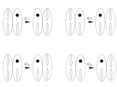
FIG. 6.: Possible interactions between a hole and a doubly occupied rung. Each process is labeled by the prefactor of the terms in the Hamiltonian (30) which describes it. The possible processes are: exchange with a singlet ($c_{1}$), exchange with a singlet which is transformed into a triplet ($c_{2}$), exchange with a triplet whereby the triplet remains unchanged ($c_{3}$), exchange with a triplet whereby the triplet changes its $S_{z}$ ($c_{4}$).

the hopping term a singly occupied rung can exchange its position with a ‘fully occupied’ rung. Thereby the fully occupied rung can remain in a singlet, change from singlet to triplet (and vice versa), remain in a given triplet state, or remain in a triplet state but change its $S_{z}$. These processes can be described by the following coupling terms, whose form follows simply from the requirements of spin rotation invariance, even parity, and Hermiticity:

$$H = c_{1}\sum_{n,k_{y}}[\;\bar{n}_{n}a_{n,k_{y},\sigma}^{\dagger}a_{n-1,k_{y},\sigma}+H.c.\;]$$ (27)

$$+ c_{2}\sum_{n}[\;\mathchoice{{\hbox{\boldmath$\displaystyle t$}}}{{\hbox{\boldmath$\textstyle t$}}}{{\hbox{\boldmath$\scriptstyle t$}}}{{\hbox{\boldmath$\scriptscriptstyle t$}}}_{n}^{\dagger}\cdot(\bar{n}_{n+1}\mathchoice{{\hbox{\boldmath$\displaystyle S$}}}{{\hbox{\boldmath$\textstyle S$}}}{{\hbox{\boldmath$\scriptstyle S$}}}{{\hbox{\boldmath$\scriptscriptstyle S$}}}_{n,n+1}+\bar{n}_{n-1}\mathchoice{{\hbox{\boldmath$\displaystyle S$}}}{{\hbox{\boldmath$\textstyle S$}}}{{\hbox{\boldmath$\scriptstyle S$}}}{{\hbox{\boldmath$\scriptscriptstyle S$}}}_{n,n-1})+H.c.]$$ (28)

$$+ c_{3}\sum_{n}[\;\mathchoice{{\hbox{\boldmath$\displaystyle t$}}}{{\hbox{\boldmath$\textstyle t$}}}{{\hbox{\boldmath$\scriptstyle t$}}}{{\hbox{\boldmath$\scriptscriptstyle t$}}}_{n-1}^{\dagger}\cdot\mathchoice{{\hbox{\boldmath$\displaystyle t$}}}{{\hbox{\boldmath$\textstyle t$}}}{{\hbox{\boldmath$\scriptstyle t$}}}{{\hbox{\boldmath$\scriptscriptstyle t$}}}_{n}\;\sum_{k_{y},\sigma}a_{n,k_{y},\sigma}^{\dagger}a_{n-1,k_{y},\sigma}+H.c.\;]$$ (29)

$$+ c_{4}\sum_{n}[\;i\bar{\mathchoice{{\hbox{\boldmath$\displaystyle S$}}}{{\hbox{\boldmath$\textstyle S$}}}{{\hbox{\boldmath$\scriptstyle S$}}}{{\hbox{\boldmath$\scriptscriptstyle S$}}}}_{n,n-1}\cdot(\mathchoice{{\hbox{\boldmath$\displaystyle t$}}}{{\hbox{\boldmath$\textstyle t$}}}{{\hbox{\boldmath$\scriptstyle t$}}}{{\hbox{\boldmath$\scriptscriptstyle t$}}}_{n}^{\dagger}\times\mathchoice{{\hbox{\boldmath$\displaystyle t$}}}{{\hbox{\boldmath$\textstyle t$}}}{{\hbox{\boldmath$\scriptstyle t$}}}{{\hbox{\boldmath$\scriptscriptstyle t$}}}_{n-1})+H.c.\;],$$ (30)

where

$\displaystyle\bar{n}_{n}=1-\mathchoice{{\hbox{\boldmath$\displaystyle t$}}}{{\hbox{\boldmath$\textstyle t$}}}{{\hbox{\boldmath$\scriptstyle t$}}}{{\hbox{\boldmath$\scriptscriptstyle t$}}}_{n}^{\dagger}\cdot\mathchoice{{\hbox{\boldmath$\displaystyle t$}}}{{\hbox{\boldmath$\textstyle t$}}}{{\hbox{\boldmath$\scriptstyle t$}}}{{\hbox{\boldmath$\scriptscriptstyle t$}}}_{n}.$

To determine the numerical values of the coefficients $c_{i}$ we start with the state $|1\rangle=a_{1,k_{y},\uparrow}^{\dagger}s_{2}^{\dagger}|vac\rangle$. Denoting the hopping term along the legs by $H_{t}$ we find:

$\displaystyle H_{t}|1\rangle=\frac{t}{2}(a_{2,k_{y},\uparrow}^{\dagger}s_{1}^{\dagger}+a_{2,k_{y}+\pi,\uparrow}^{\dagger}t_{1,z}^{\dagger}-\sqrt{2}a_{2,k_{y}+\pi,\downarrow}^{\dagger}t_{1,+}^{\dagger})|vac\rangle.$

Next, starting from the state $|1^{\prime}\rangle=a_{1,k_{y},\uparrow}^{\dagger}t_{2,z}^{\dagger}|vac\rangle$ we obtain

$\displaystyle H_{t}|1^{\prime}\rangle=\frac{t}{2}(a_{2,k_{y}+\pi,\uparrow}^{\dagger}s_{1}^{\dagger}+a_{2,k_{y},\uparrow}^{\dagger}t_{1,z}^{\dagger}+\sqrt{2}a_{2,k_{y},\downarrow}^{\dagger}t_{1,+}^{\dagger})|vac\rangle.$

Using these two equations we find $c_{1}$$=$$t/2$, $c_{2}$$=$$t$, $c_{3}$$=$$t/2$, and $c_{4}$$=$$-t$.
Next, we consider the action of the exchange terms along the legs. Namely the electron on a singly occupied rung can exchange with an electron belonging to a singlet or triplet on a neighboring rung. Again we can write down the general form of the Hamiltonian as

$$H = c_{2}^{\prime}\sum_{n}[\;(\mathchoice{{\hbox{\boldmath$\displaystyle t$}}}{{\hbox{\boldmath$\textstyle t$}}}{{\hbox{\boldmath$\scriptstyle t$}}}{{\hbox{\boldmath$\scriptscriptstyle t$}}}_{n+1}^{\dagger}+\mathchoice{{\hbox{\boldmath$\displaystyle t$}}}{{\hbox{\boldmath$\textstyle t$}}}{{\hbox{\boldmath$\scriptstyle t$}}}{{\hbox{\boldmath$\scriptscriptstyle t$}}}_{n-1}^{\dagger})\cdot\mathchoice{{\hbox{\boldmath$\displaystyle S$}}}{{\hbox{\boldmath$\textstyle S$}}}{{\hbox{\boldmath$\scriptstyle S$}}}{{\hbox{\boldmath$\scriptscriptstyle S$}}}_{n,n}+H.c.]$$ (31)

$$+ c_{4}^{\prime}\sum_{n}\;i\bar{\mathchoice{{\hbox{\boldmath$\displaystyle S$}}}{{\hbox{\boldmath$\textstyle S$}}}{{\hbox{\boldmath$\scriptstyle S$}}}{{\hbox{\boldmath$\scriptscriptstyle S$}}}}_{n,n}\cdot(\mathchoice{{\hbox{\boldmath$\displaystyle t$}}}{{\hbox{\boldmath$\textstyle t$}}}{{\hbox{\boldmath$\scriptstyle t$}}}{{\hbox{\boldmath$\scriptscriptstyle t$}}}_{n\pm 1}^{\dagger}\times\mathchoice{{\hbox{\boldmath$\displaystyle t$}}}{{\hbox{\boldmath$\textstyle t$}}}{{\hbox{\boldmath$\scriptstyle t$}}}{{\hbox{\boldmath$\scriptscriptstyle t$}}}_{n\pm 1}).$$ (32)

Denoting the exchange term along the legs as $H_{J}$, we find

$$H_{J}|1\rangle = \frac{J}{4}(a_{1,k_{y}+\pi,\uparrow}^{\dagger}t_{2,z}^{\dagger}-\sqrt{2}a_{1,k_{y}+\pi,\downarrow}^{\dagger}t_{2,+}^{\dagger})|vac\rangle,$$ (33)

$$H_{J}|1^{\prime}\rangle = \frac{J}{4}(a_{1,k_{y}+\pi,\uparrow}^{\dagger}s_{2}^{\dagger}+\sqrt{2}a_{1,k_{y},\downarrow}^{\dagger}t_{2,+}^{\dagger})|vac\rangle,$$ (34)

whence $c_{2}^{\prime}$$=$$J/2$ and $c_{4}^{\prime}$$=$$-J/2$. Together with the Hamiltonian for the triplet-dynamics, Eq. (12) then gives a complete description for the hole motion in the ladder.
Having found all possible ways of interaction between the hole and the spin excitations, we need to consider a suitable approximation to handle these terms. To begin with, by treating the terms $\propto c_{1},c_{2}$ in (30) in a mean-field like way, we may hope to obtain a ‘renormalized hopping’ integral for the hole. Namely we replace $\bar{n}_{n}\rightarrow(1-n_{b})$, with $n_{b}=0.3$ the density of triplets (see above). Next, in the term $\propto c_{3}$ we replace

$$\mathchoice{{\hbox{\boldmath$\displaystyle t$}}}{{\hbox{\boldmath$\textstyle t$}}}{{\hbox{\boldmath$\scriptstyle t$}}}{{\hbox{\boldmath$\scriptscriptstyle t$}}}_{n-1}^{\dagger}\cdot\mathchoice{{\hbox{\boldmath$\displaystyle t$}}}{{\hbox{\boldmath$\textstyle t$}}}{{\hbox{\boldmath$\scriptstyle t$}}}{{\hbox{\boldmath$\scriptscriptstyle t$}}}_{n} \rightarrow \langle\mathchoice{{\hbox{\boldmath$\displaystyle t$}}}{{\hbox{\boldmath$\textstyle t$}}}{{\hbox{\boldmath$\scriptstyle t$}}}{{\hbox{\boldmath$\scriptscriptstyle t$}}}_{n-1}^{\dagger}\cdot\mathchoice{{\hbox{\boldmath$\displaystyle t$}}}{{\hbox{\boldmath$\textstyle t$}}}{{\hbox{\boldmath$\scriptstyle t$}}}{{\hbox{\boldmath$\scriptscriptstyle t$}}}_{n}\rangle$$ (35)

$$= \frac{3}{N}\sum_{k}\cos(k)\;v_{k}^{2}.$$ (36)

We thus obtain the ‘effective hopping integral’

$\displaystyle t_{eff}=\frac{t}{2}[\;(1-n_{b})+\frac{3}{N}\sum_{k}\cos(k)\;v_{k}^{2}\;].$

Numerical evaluation shows that this is a very small quantity, $t_{eff}$$=$$0.27t$, the reason being that the second term on the r.h.s. is negative and of quite appreciable magnitude.
The form of the terms $\propto c_{2},c_{2}^{\prime}$ suggests the ‘rainbow diagram’ approximation due to Schmidt-Rink et al.[13] to treat them. This still leaves us with the terms $\propto c_{4},c_{4}^{\prime}$; detailed investigation shows, however, that the matrix elements of these terms are proportional to higher powers of the (small) coherence factor $v_{k}$; we take this as a justification to neglect these terms.
Next, we briefly discuss additional ‘renormalizations’ which might occur. In the same way as a triplet on some given rung will ‘block’ quantum fluctuations and hamper the propagation of other triplets, a singly occupied rung will do the same. For the triplets, this effect has led to a quite dramatic increase of the ‘energy of formation’ of the triplet. However, the corresponding renormalization of the on-site energy for the hole-like Fermions is most likely independent of the $k_{y}$ of the hole, and hence can be absorbed into an overall constant shift of the spectral function. Since, the hole will not be able to propagate by two lattice sites by coupling to a quantum fluctuation, so that we expect that unlike the case of spin excitations there will be no ‘dynamically generated’ next-nearest neighbor hopping.
Performing the Fourier and Bogoliubov transform we finally arrive at the following Hamiltonian

$$H = \sum_{\mathchoice{{\hbox{\boldmath$\displaystyle k$}}}{{\hbox{\boldmath$\textstyle k$}}}{{\hbox{\boldmath$\scriptstyle k$}}}{{\hbox{\boldmath$\scriptscriptstyle k$}}},\sigma}\epsilon_{\mathchoice{{\hbox{\boldmath$\displaystyle k$}}}{{\hbox{\boldmath$\textstyle k$}}}{{\hbox{\boldmath$\scriptstyle k$}}}{{\hbox{\boldmath$\scriptscriptstyle k$}}}}a_{\mathchoice{{\hbox{\boldmath$\displaystyle k$}}}{{\hbox{\boldmath$\textstyle k$}}}{{\hbox{\boldmath$\scriptstyle k$}}}{{\hbox{\boldmath$\scriptscriptstyle k$}}},\sigma}^{\dagger}a_{\mathchoice{{\hbox{\boldmath$\displaystyle k$}}}{{\hbox{\boldmath$\textstyle k$}}}{{\hbox{\boldmath$\scriptstyle k$}}}{{\hbox{\boldmath$\scriptscriptstyle k$}}},\sigma}+\sum_{\mathchoice{{\hbox{\boldmath$\displaystyle q$}}}{{\hbox{\boldmath$\textstyle q$}}}{{\hbox{\boldmath$\scriptstyle q$}}}{{\hbox{\boldmath$\scriptscriptstyle q$}}}}\omega_{\mathchoice{{\hbox{\boldmath$\displaystyle q$}}}{{\hbox{\boldmath$\textstyle q$}}}{{\hbox{\boldmath$\scriptstyle q$}}}{{\hbox{\boldmath$\scriptscriptstyle q$}}}}\mathchoice{{\hbox{\boldmath$\displaystyle\gamma$}}}{{\hbox{\boldmath$\textstyle\gamma$}}}{{\hbox{\boldmath$\scriptstyle\gamma$}}}{{\hbox{\boldmath$\scriptscriptstyle\gamma$}}}_{\mathchoice{{\hbox{\boldmath$\displaystyle q$}}}{{\hbox{\boldmath$\textstyle q$}}}{{\hbox{\boldmath$\scriptstyle q$}}}{{\hbox{\boldmath$\scriptscriptstyle q$}}}}^{\dagger}\mathchoice{{\hbox{\boldmath$\displaystyle\gamma$}}}{{\hbox{\boldmath$\textstyle\gamma$}}}{{\hbox{\boldmath$\scriptstyle\gamma$}}}{{\hbox{\boldmath$\scriptscriptstyle\gamma$}}}_{\mathchoice{{\hbox{\boldmath$\displaystyle q$}}}{{\hbox{\boldmath$\textstyle q$}}}{{\hbox{\boldmath$\scriptstyle q$}}}{{\hbox{\boldmath$\scriptscriptstyle q$}}}}$$ (37)

$$+ \frac{1}{\sqrt{N}}\sum_{\mathchoice{{\hbox{\boldmath$\displaystyle k$}}}{{\hbox{\boldmath$\textstyle k$}}}{{\hbox{\boldmath$\scriptstyle k$}}}{{\hbox{\boldmath$\scriptscriptstyle k$}}},\mathchoice{{\hbox{\boldmath$\displaystyle q$}}}{{\hbox{\boldmath$\textstyle q$}}}{{\hbox{\boldmath$\scriptstyle q$}}}{{\hbox{\boldmath$\scriptscriptstyle q$}}}}\;[\;m(\mathchoice{{\hbox{\boldmath$\displaystyle k$}}}{{\hbox{\boldmath$\textstyle k$}}}{{\hbox{\boldmath$\scriptstyle k$}}}{{\hbox{\boldmath$\scriptscriptstyle k$}}},\mathchoice{{\hbox{\boldmath$\displaystyle q$}}}{{\hbox{\boldmath$\textstyle q$}}}{{\hbox{\boldmath$\scriptstyle q$}}}{{\hbox{\boldmath$\scriptscriptstyle q$}}})\;\mathchoice{{\hbox{\boldmath$\displaystyle\gamma$}}}{{\hbox{\boldmath$\textstyle\gamma$}}}{{\hbox{\boldmath$\scriptstyle\gamma$}}}{{\hbox{\boldmath$\scriptscriptstyle\gamma$}}}_{\mathchoice{{\hbox{\boldmath$\displaystyle q$}}}{{\hbox{\boldmath$\textstyle q$}}}{{\hbox{\boldmath$\scriptstyle q$}}}{{\hbox{\boldmath$\scriptscriptstyle q$}}}}^{\dagger}\cdot\mathchoice{{\hbox{\boldmath$\displaystyle S$}}}{{\hbox{\boldmath$\textstyle S$}}}{{\hbox{\boldmath$\scriptstyle S$}}}{{\hbox{\boldmath$\scriptscriptstyle S$}}}_{\mathchoice{{\hbox{\boldmath$\displaystyle k$}}}{{\hbox{\boldmath$\textstyle k$}}}{{\hbox{\boldmath$\scriptstyle k$}}}{{\hbox{\boldmath$\scriptscriptstyle k$}}},\mathchoice{{\hbox{\boldmath$\displaystyle k$}}}{{\hbox{\boldmath$\textstyle k$}}}{{\hbox{\boldmath$\scriptstyle k$}}}{{\hbox{\boldmath$\scriptscriptstyle k$}}}-\mathchoice{{\hbox{\boldmath$\displaystyle q$}}}{{\hbox{\boldmath$\textstyle q$}}}{{\hbox{\boldmath$\scriptstyle q$}}}{{\hbox{\boldmath$\scriptscriptstyle q$}}}}+H.c.\;]$$ (38)

$$\epsilon_{\mathchoice{{\hbox{\boldmath$\displaystyle k$}}}{{\hbox{\boldmath$\textstyle k$}}}{{\hbox{\boldmath$\scriptstyle k$}}}{{\hbox{\boldmath$\scriptscriptstyle k$}}}} = 2t_{eff}\;\cos(k_{x})-t_{\perp}\cos(k_{y}),$$ (39)

$$m(\mathchoice{{\hbox{\boldmath$\displaystyle k$}}}{{\hbox{\boldmath$\textstyle k$}}}{{\hbox{\boldmath$\scriptstyle k$}}}{{\hbox{\boldmath$\scriptscriptstyle k$}}},\mathchoice{{\hbox{\boldmath$\displaystyle q$}}}{{\hbox{\boldmath$\textstyle q$}}}{{\hbox{\boldmath$\scriptstyle q$}}}{{\hbox{\boldmath$\scriptscriptstyle q$}}}) = \delta_{q_{y},\pi}\;[\;(2t\cos(k_{x}-q_{x})+J\cos(q_{x}))u_{q_{x}}$$ (40)

$$\;\;\;\;\;\;-(2t\cos(k_{x})+J\cos(q_{x}))v_{q_{x}}\;].$$ (41)

Thereby it is understood that $\omega_{\mathchoice{{\hbox{\boldmath$\displaystyle q$}}}{{\hbox{\boldmath$\textstyle q$}}}{{\hbox{\boldmath$\scriptstyle q$}}}{{\hbox{\boldmath$\scriptscriptstyle q$}}}}$ has only one branch with $q_{y}$$=$$0$. Formally, this is already very similar to the Hamiltonian derived by Schmidt-Rink et al.[13] for hole motion in a Heisenberg antiferromagnet; the only differences are that we have spinful holes, a nonvanishing dispersion $\epsilon_{\mathchoice{{\hbox{\boldmath$\displaystyle k$}}}{{\hbox{\boldmath$\textstyle k$}}}{{\hbox{\boldmath$\scriptstyle k$}}}{{\hbox{\boldmath$\scriptscriptstyle k$}}}}$ already for the ‘bare holes’, and $3$ branches of spin excitations rather than $1$. In short, the Hamiltonian is explicitely spin-rotation invariant, as it has to be in a ‘spin liquid’. Technically this does not make any difference and the equation for the self-energy $\Sigma(\mathchoice{{\hbox{\boldmath$\displaystyle k$}}}{{\hbox{\boldmath$\textstyle k$}}}{{\hbox{\boldmath$\scriptstyle k$}}}{{\hbox{\boldmath$\scriptscriptstyle k$}}},\omega)$ reads now

$$\Sigma(\mathchoice{{\hbox{\boldmath$\displaystyle k$}}}{{\hbox{\boldmath$\textstyle k$}}}{{\hbox{\boldmath$\scriptstyle k$}}}{{\hbox{\boldmath$\scriptscriptstyle k$}}},\omega)=\frac{3}{N}\sum_{\mathchoice{{\hbox{\boldmath$\displaystyle q$}}}{{\hbox{\boldmath$\textstyle q$}}}{{\hbox{\boldmath$\scriptstyle q$}}}{{\hbox{\boldmath$\scriptscriptstyle q$}}}}\frac{|m(\mathchoice{{\hbox{\boldmath$\displaystyle k$}}}{{\hbox{\boldmath$\textstyle k$}}}{{\hbox{\boldmath$\scriptstyle k$}}}{{\hbox{\boldmath$\scriptscriptstyle k$}}},\mathchoice{{\hbox{\boldmath$\displaystyle q$}}}{{\hbox{\boldmath$\textstyle q$}}}{{\hbox{\boldmath$\scriptstyle q$}}}{{\hbox{\boldmath$\scriptscriptstyle q$}}})|^{2}}{\omega-\epsilon_{\mathchoice{{\hbox{\boldmath$\displaystyle k$}}}{{\hbox{\boldmath$\textstyle k$}}}{{\hbox{\boldmath$\scriptstyle k$}}}{{\hbox{\boldmath$\scriptscriptstyle k$}}}-\mathchoice{{\hbox{\boldmath$\displaystyle q$}}}{{\hbox{\boldmath$\textstyle q$}}}{{\hbox{\boldmath$\scriptstyle q$}}}{{\hbox{\boldmath$\scriptscriptstyle q$}}}}-\omega_{\mathchoice{{\hbox{\boldmath$\displaystyle q$}}}{{\hbox{\boldmath$\textstyle q$}}}{{\hbox{\boldmath$\scriptstyle q$}}}{{\hbox{\boldmath$\scriptscriptstyle q$}}}}-\Sigma(\mathchoice{{\hbox{\boldmath$\displaystyle k$}}}{{\hbox{\boldmath$\textstyle k$}}}{{\hbox{\boldmath$\scriptstyle k$}}}{{\hbox{\boldmath$\scriptscriptstyle k$}}}-\mathchoice{{\hbox{\boldmath$\displaystyle q$}}}{{\hbox{\boldmath$\textstyle q$}}}{{\hbox{\boldmath$\scriptstyle q$}}}{{\hbox{\boldmath$\scriptscriptstyle q$}}},\omega)}.$$ (42)

The self-consistency equation can be solved for relatively large systems (we used $N=$$200$), and the self-energy be used to calculate the hole-like photoemission spectrum

$$A(\mathchoice{{\hbox{\boldmath$\displaystyle k$}}}{{\hbox{\boldmath$\textstyle k$}}}{{\hbox{\boldmath$\scriptstyle k$}}}{{\hbox{\boldmath$\scriptscriptstyle k$}}},\omega)=-\frac{1}{\pi}\Im\frac{1}{-\omega-\epsilon_{\mathchoice{{\hbox{\boldmath$\displaystyle k$}}}{{\hbox{\boldmath$\textstyle k$}}}{{\hbox{\boldmath$\scriptstyle k$}}}{{\hbox{\boldmath$\scriptscriptstyle k$}}}}-\Sigma(\mathchoice{{\hbox{\boldmath$\displaystyle k$}}}{{\hbox{\boldmath$\textstyle k$}}}{{\hbox{\boldmath$\scriptstyle k$}}}{{\hbox{\boldmath$\scriptscriptstyle k$}}},\omega)+i0^{+}}.$$ (43)

If we want to compare this spectrum with Lanczos results[12], some care is necessary. The reason is that the spectral function we have calculated above is the one for the creation of a ‘bare’ hole. When calculating the photoemission spectrum, i.e. the spectral function of the operator $c_{\mathchoice{{\hbox{\boldmath$\displaystyle k$}}}{{\hbox{\boldmath$\textstyle k$}}}{{\hbox{\boldmath$\scriptstyle k$}}}{{\hbox{\boldmath$\scriptscriptstyle k$}}},\sigma}$, there exists the possibility that the annihilation operator ‘hits’ a rung in a triplet state. This will lead to terms of the form $a_{\mathchoice{{\hbox{\boldmath$\displaystyle k$}}}{{\hbox{\boldmath$\textstyle k$}}}{{\hbox{\boldmath$\scriptstyle k$}}}{{\hbox{\boldmath$\scriptscriptstyle k$}}}+\mathchoice{{\hbox{\boldmath$\displaystyle q$}}}{{\hbox{\boldmath$\textstyle q$}}}{{\hbox{\boldmath$\scriptstyle q$}}}{{\hbox{\boldmath$\scriptscriptstyle q$}}},\sigma}^{\dagger}t_{\mathchoice{{\hbox{\boldmath$\displaystyle q$}}}{{\hbox{\boldmath$\textstyle q$}}}{{\hbox{\boldmath$\scriptstyle q$}}}{{\hbox{\boldmath$\scriptscriptstyle q$}}}}$ in the photoemission operator, i.e. the creation of the hole is accompanied by the annihilation of a spin excitation. If we want to have numerical results for the bare hole spectral function, we therefore should use the Fourier transform of the operator

$$\tilde{c}_{n,k_{y},\uparrow} = a_{n,k_{y},\downarrow}^{\dagger}s_{n,n+\hat{y}}$$ (44)

$$= \frac{1}{2}[\;(\;c_{n,\uparrow}n_{n+\hat{y},\downarrow}-c_{n,\downarrow}S_{n+\hat{y}}^{-}\;)$$ (45)

$$\;\;\;\;+e^{ik_{y}}(\;c_{n+\hat{y},\uparrow}n_{n,\downarrow}-c_{n+\hat{y},\downarrow}S_{n}^{-}\;)\;].$$ (46)

This operator replaces a rung-singlet by a singly occupied bond with the proper $k_{y}$, and annihilates any triplet. This may therefore be considered as a creation operator for a ‘bare’ hole. Then, Figure (7) compares the ‘bare hole’ spectral function obtained by the self-consistent Born approximation and the Lanczos spectra of the operator $\tilde{c}_{\mathchoice{{\hbox{\boldmath$\displaystyle k$}}}{{\hbox{\boldmath$\textstyle k$}}}{{\hbox{\boldmath$\scriptstyle k$}}}{{\hbox{\boldmath$\scriptscriptstyle k$}}},\sigma}$. The agreement is obviously quite good, although the self-consistent Born result tends to produce ‘too coherent’ spectra and does not put enough weight

FIG. 7.: Hole spectral function by self-consistent Born aproximation (full line) compared to the spectrum of $\tilde{c}_{\mathchoice{{\hbox{\boldmath$\displaystyle k$}}}{{\hbox{\boldmath$\textstyle k$}}}{{\hbox{\boldmath$\scriptstyle k$}}}{{\hbox{\boldmath$\scriptscriptstyle k$}}},\sigma}$ obtained by Lanczos diagonalization in a $2\times 10$ ladder (dotted line). The ratio $J/t$$=$$0.5$.

into incoherent continua. This may be an indication that our renormalization of the coupling matrix element $m(\mathchoice{{\hbox{\boldmath$\displaystyle k$}}}{{\hbox{\boldmath$\textstyle k$}}}{{\hbox{\boldmath$\scriptstyle k$}}}{{\hbox{\boldmath$\scriptscriptstyle k$}}},\mathchoice{{\hbox{\boldmath$\displaystyle q$}}}{{\hbox{\boldmath$\textstyle q$}}}{{\hbox{\boldmath$\scriptstyle q$}}}{{\hbox{\boldmath$\scriptscriptstyle q$}}})$ by $(1-n_{b})$ is too strong - a larger coupling would presumably lead to more incoherent weight. The key features, however, are essentially identical in both spectra: the intense band in the $k_{y}$$=$$0$ sector, which disperses slightly upwards from $k$$=$$0$ towards $k$$=$$\pi/2$ and then more or less levels off; the equally intense band in the $k_{y}=\pi$ sector, which starts out at $k$$=$$\pi$, disperses towards lower energy and quickly becomes ‘overdamped’. The SCB results somewhat underestimate the bandwidth of the $k_{y}$$=$$0$ quasiparticle band and put the $k_{y}$$=$$0$ at a somewhat too high energy. The former could probably be remedied by adjustment of the ‘bare hole hopping integral’ $t_{eff}$ - however, since there is no rigorous way to do so, we decided not to do this. Apart from these relatively minor problems, however, there is quite good agreement.
As a last remark we note that a comparison with the ‘full’ photoemission spectrum[12] shows quite substantial differences in the spectral weight of some features. The additional processes where the photoemission operator annihilates a quantum fluctuation (in this case a triplet) thus are quite important for a discussion of the true photoemission lineshape (see also Refs. [14, 15] for a discussion of this issue in the 2D systems).

IV Conclusion

In summary, we have derived a simple theory of two-legged spin ladders which reproduces a number of numerical results quite well. Being of comparable simplicity as linear spin wave theory for the planar Heisenberg antiferromagnet, the theory nevertheless allows to make quantitative calculations of physical quantities, which in all cases compare favourably with the results of Lanczos diagonalization. Just as linear spin wave theory may be viewed as constructing an effective Hamiltonian for the pair creation and propagation of fluctuations around the ‘Neel-vacuum’, the present theory may be viewed as an entirely analogous expansion around the ‘RVB-vacuum’: the Hamiltonians (8) and (12) may be thought of as describing the dynamics of triplet-like fluctuations around the RVB vacuum, and to discuss the hole dynamics we basically needed to describe the coupling between these triplet-excitations and the doped hole. The great simplification which made the calculation possible was the special geometry of the $2$-legged ladder which immediately suggested a unique RVB-vacuum around which we could ‘expand’ the fluctuating ground state. We note that there actually exists another system with such a unique RVB-vacuum, namely the Kondo lattice. For this system an analogous procedure involving Fermionic fluctuations is possible and leads to excellent results when compared to Lanczos diagonalization[16].
In a two dimensional $t-J$-like system, such a unique vacuum does in general not exist, unless one were to assume some spatial inhomogeneities such as stripes[17]. Rather, for a translationally invariant state, the most natural vacuum would be a statistical average over all possible dimer-coverings of the plane, where each dimer corresponds to a singlet[18]. The analogue of the triplet-like excitations in the ladder then would be states where one or several singlet-dimers are substituted by a triplet, and this excited dimer propagates through the system. In fact, up to an additional statistical averaging to account for the probability of suitable dimer configurations, the calculation of matrix elements for the pair creation and propagation of these excited dimers proceeds in an entirely analogous way as for the ladder[19]. We note that such a picture for the low energy excitations of the RVB state is almost mandatory in the framework of the $SO(5)$ symmetric theory of cuprate superconductors by Zhang[20]: there, the $\pi$-operator, which actually accomplishes the $SO(5)$ rotations of spin-excited, half-filled states into doped, superconducting ground states[21] precisely converts excited dimers with momentum $(\pi,\pi)$ into $d_{x^{2}-y^{2}}$ symmetric hole pairs with momentum $(0,0)$. Then, the simplest picture of the SO(5) rotation from the antiferromagnetic to the superconducting state[20] would be that a condensate of excited dimers with momentum $(\pi,\pi)$ at half-filling (i.e. a state with nonvanishing staggered magnetization) is converted into a condensate of $d$-like hole pairs (i.e. a $d$-wave superconductor) in the doped case. A description of the spin excitations in $2D$ in terms of Boson-like excited dimers as for the $t-J$ ladder thus may be a very natural starting point for this promising scenario.
Instructive discussions with Dr O. P. Sushkov and Dr E. Arrigoni are most gratefully acknowledged.

TABLE I.: The Fourier coefficients of the renormalized energy $\tilde{\epsilon}_{k}$ and pairing amplitude $\tilde{\Delta}_{k}$, extrapolated to infinite length of the ladder.

	0	1	2
$\tilde{\epsilon}_{k}$	1.77	0.21	-0.32
$\tilde{\Delta}_{k}$	0.07	1.03	-0.17

REFERENCES

• [1] Z. Hiroi, M. Azuma, M. Takano, and Y. Bando, J. Solid State Chem. 95, 230, (1991).
• [2] E. Dagotto and T. M. Rice, Science 271, 618 (1996).
• [3] M. Azuma, Z. Hiroi, M. Takano, K. Ishida, and Y. Kitaoka, Phys. Rev. Lett. 73, 3463 (1994).
• [4] M. Uehara, T. Nagata, J. Akimitsu, H. Takahashi, N. Mori,, and K. Kinoshita, J. Phys. Soc. Jpn. 65, 2764 (1996).
• [5] S. Gopalan, T. M. Rice, and M. Sigrist, Phys. Rev. B 49, 8901 (1994).
• [6] H. Endres, R. M. Noack, W. Hanke, D. Poilblanc, and D. J. Scalapino, Phys. Rev. B 53, 5530 (1996).
• [7] G. Sierra and M. A. Martin-Delgado, Phys. Rev. B 56, 8774 (1996); G. Sierra, M.A. Martin-Delgado, J. Dukelsky, S.R. White, and D.J. Scalapino, cond-mat/9707335.
• [8] E. Dagotto, G. B. Martins, J. Piekarewicz, and J. R. Shepard, cond-mat/9707205.
• [9] T. Barnes and J. Riera, Phys. Rev. B 50, 6817 (1994).
• [10] S. R. White, R. M. Noack, and D. J. Scalapino, Phys. Rev. Lett. 73, 886 (1994).
• [11] J. Lorenzana and G. A. Sawatzky, Phys. Rev. Lett. 74, 1867 (1995).
• [12] S. Haas and E. Dagotto, Phys. Rev. B 54, R3718 (1996).
• [13] S. Schmidt-Rink, C. M. Varma, and A. E. Ruckenstein, Phys. Rev. Lett. 60, 2793 (1988).
• [14] R. Eder and K. W. Becker, Phys. Rev. B 44, 6982 (1991).
• [15] O. P. Sushkov, G. A. Sawatzky, R. Eder, and H. Eskes, Phys. Rev. B 56, 11769 (1997).
• [16] R. Eder, O. Stoica, and G. Sawatzky, Phys. Rev. B. 55, R6109 (1997); R. Eder, O. Rogojanu, and G. A. Sawatzky, preprint cond-mat/9711248.
• [17] H. Eskes, R. Grimberg, W. van Saaloss, and J. Zaanen, Phys. Rev. B 54, R724 (1996).
• [18] B. Sutherland, Phys. Rev. B 37, 3786 (1988).
• [19] R. Eder, unpublished.
• [20] S.C. Zhang, Science 275, 1089 (1997).
• [21] R. Eder, W. Hanke, and S. C. Zhang, preprint cond-mat/9707233.