Quantum Kinetic Theory III: Quantum kinetic master equation for strongly condensed trapped systems

Abstract

We extend quantum kinetic theory to deal with a strongly Bose-condensed atomic vapor in a trap. The method assumes that the majority of the vapor is not condensed, and acts as a bath of heat and atoms for the condensate. The condensate is described by the particle number conserving Bogoliubov method developed by one of the authors. We derive equations which describe the fluctuations of particle number and phase, and the growth of the Bose-Einstein condensate. The equilibrium state of the condensate is a mixture of states with different numbers of particles and quasiparticles. It is not a quantum superposition of states with different numbers of particles—nevertheless, the stationary state exhibits the property of off-diagonal long range order, to the extent that this concept makes sense in a tightly trapped condensate.

I Introduction

In two previous papers on quantum kinetic theory, which we shall call QKI [1] and QKII [2] in this paper, we focussed on the theory of a Bose gas in which there was

• No more than a small amount of Bose condensate, so that the interactions between the particles were not sufficiently strong to produce a significant modification to the excitation spectrum of the Bose gas;

• No trapping potential, so that the system was spatially homogeneous.

Such a treatment gives insight into the the statistical aspects of quantum kinetics, but cannot be applied to the condensates presently being produced [3, 4, 5, 6, 7, 8], in which there is very strong condensation of an alkali metal vapor in a rather tight trap.

In this work the focus will be on strongly condensed trapped systems, with a methodology based on that of QKI, but somewhat simplified in order to exhibit the major features of the interaction of a Bose-condensate with a vapor of non-condensed particles. The basis of our method is to divide the condensate spectrum into two bands; the condensate band, in which the presence of the condensate significantly modifies the excitation spectrum, and the non-condensate band, whose energy levels are sufficiently high for the interaction with the condensate to be negligible.

In Fig.1(a) we depict the kind of trap for which this division is very clear—a rather wide trap, in the center of which is a small tight trap, with a few energy levels. In contrast, in Fig.1(b) we depict a harmonic trap, in which the division is not so obvious. In fact, however, the three dimensional nature of the trap, in which the density of states increases quadratically with energy, also yields a relatively small number of isolated levels at low energies, which rapidly approaches a continuum, so the dramatic difference between the two traps is more apparent than real. Current experiments all use harmonic traps, but the “ideal” trap of Fig.1(b) would in principle be better adapted to studies of the condensate itself.

The dynamics of the non-condensate band is thus well described by the kind of formalism used in QKI, with modifications to take account of the fact that we have also introduced a trapping potential $V_{T}({\bf x})$. On the other hand, the dynamics of the condensate band is well described by the energy spectrum which arises from Bogoliubov’s method [9], as adapted to apply to the case of particles in a trap [10]. This kind of dynamics has been well studied by many workers in the past two years [10, 11, 22], and the equation of motion for the condensate wavefunction is now generally verified both theoretically and experimentally to be the time-dependent Gross-Pitaveskii equation [12].

The aim of this paper is to develop and use methods to describe the interaction between the condensate band and the non-condensate band. The results of our investigations can be summarized as follows:

• The non-condensate band is taken to be fully thermalized, in the sense that at any point ${\bf u},{\bf k}$ in phase space there is a local particle phase-space density $F({\bf u},{\bf k})$, and the space time correlation functions of this phase space density have a weakly damped classical form.

• The dynamics of the condensate band, in interaction with the thermalized non-condensate band, is given by a master equation (83–88), in which the interaction terms are of three kinds:

  • Two particles in the non-condensate band collide, and after the collision, one of these particle remains within the condensate band; and there is also of course the corresponding time-reversed process.

  • A particle in the non-condensate band collides with a particle in the condensate band, and exchanges energy with it, but does not enter the condensate band.

  • A particle in the non-condensate band collides with one in the condensate band, and after the collision both particles are left in the condensate band; and again there is also of course the corresponding time-reversed process.

• By using the particle-number-conserving Bogoliubov method [18] developed by one of us, the expressions which arise in the master equation can be re-written in a form in which the processes are described in terms of

  • Creation and destruction of particles; thus if $N$ is the total number of particles in the condensate band, we introduce operators $A^{\dagger},A$ which change $N$ by $\pm 1$.

  • Creation and destruction of quasiparticles, which are to be regarded as quantized oscillations of the whole body of $N$ particles in the condensate band.

  Thus there is a clear distinction made between creation and destruction of particles $(N\to N\pm 1)$, and the creation and destruction of quasiparticles, which are mere excitations, and not particles. This distinction follows from the particle number conserving Bogoliubov method [18], and has not been made clear in nearly all earlier treatments of Bogoliubov’s method, which blur this distinction, and give the misleading impression that the Bogoliubov excitation spectrum can only be obtained if strict conservation of particle number is abandoned. We emphasize here that the particle number conserving Bogoliubov method gives exactly the same results for the excitation spectrum as the usual version; however, because particle number conservation is maintained, it is possible to specify both wavefunctions and energy eigenvalues for states with a definite energy and a definite number of particles.

• It is possible to split off the largest terms in the master equation, and approximate the description by a single basic master equation for $N$, the number of particles in the condensate band, and thus arrive at a description of the growth of a condensate from the vapor. The very simplest version of this description, in which all fluctuations are neglected, takes the form of a single differential equation

  $$\dot{N}=2W^{+}(N)\left\{\left(1-e^{[\mu-\mu(N)]/k_{B}T}\right)N+1\right\}$$ (1)

  in which $W^{+}(N)$ is a certain kinetic coefficient, for which we can give an approximate form, and $\mu$ and $\mu(N)$ are respectively the vapor chemical potential and the chemical potential of the condensate wavefunction for $N$ particles, as given by solving the time-independent Gross-Pitaevskii equation.

• Detailed descriptions of the dynamics of fluctuations can be given. The stationary solution for the condensate density operator is a mixture (not a quantum-mechanical superposition) of states with different numbers $N$ of particles. For each such state, the wavefunction of the condensate is $\xi_{N}({\bf x})$, the solution of the the time-independent Gross-Pitaevskii equation for $N$ particles.

• A description of both phase diffusion of the condensate and of the decay of excitations can also be given, and these will appear in a subsequent paper. [13].

The description given in this paper is a simplified one, in which the non-condensate band is treated as stationary, so that it does constitute a genuine “heat-bath”, characterized by a fixed temperature $T$ and a fixed chemical potential $\mu$. This is not an essential feature of the basic quantum kinetic description, which, in its full form, treats the two bands as having their own dynamics as well as being coupled together. The full quantum kinetic theory will be presented in a subsequent paper, QKV. It turns out to be a rather intricate process to derive such a description, even though the essential result, as used in this paper, is that the non-condensate band is described by an equation of the Uehling-Uhlenbeck form [15], with correlation functions of a thermal form.

II Description of the system

A Hamiltonian and notation

As in QKI, we consider a set of Spin-0 Bose particles, described by the Hamiltonian

$$H=H_{\rm kin}+H_{I}+H_{T},$$ (2)

in which

$$H_{\rm kin}=\int d^{3}{\bf x}\,\psi^{\dagger}({\bf x})\left(-{\hbar^{2}\over 2m}\nabla^{2}\right)\psi({\bf x})$$ (3)

and

$$H_{I} = {1\over 2}\int d^{3}{\bf x}\int d^{3}{\bf x}^{\prime}\psi^{\dagger}({\bf x})\psi^{\dagger}({\bf x}^{\prime})u({\bf x}-{\bf x}^{\prime})\psi({\bf x}^{\prime})\psi({\bf x}).$$ (4)

The potential function $u({\bf x}-{\bf x}^{\prime})$ is a c-number and is as usual not the true interatomic potential, but rather a short range potential—approximately a delta function—which reproduces the correct scattering length. This enables the Born approximation to be applied, and thus simplifies the mathematics considerably. [17]

The term $H_{T}$ arises from a trapping potential, and is written as

$$H_{T}=\int d^{3}{\bf x}\,V_{T}({\bf x)}\psi^{\dagger}({\bf x})\psi({\bf x}).$$ (6)

Thus, this is the standard second quantized theory of an interacting Bose gas of particles with mass $m$.

B Condensate and non-condensate bands

When there is strong condensation in a trap, the lowest energy level of the trap develops a macroscopic occupation, and modifies the other energy levels in the trap. If the trap is quite tight, the lower energy levels are reasonably well separated, as is indeed experimentally the case [3, 4, 5]. The concept of a “tight” trap is however not absolute; a trap may be tight for the lower energy levels, but quite broad for the higher energy levels. The essential distinction is the density of states, which increases like $E^{2}$ for a harmonic trap, leading to very closely spaced levels for quite moderate energy. In addition, one must also note that the modification of the energy levels induced by the condensate affects only the lower levels significantly.

The procedure which follows from these is to divide the particle states into a condensate band $R_{C}$ and non condensate band $R_{NC}$, and to perform a corresponding resolution of the field operator in the form $\psi({\bf x})=\phi({\bf x})+\psi_{NC}({\bf x})$. The separation between the two bands is in terms of energy; we choose to define the division in such a way that the energies of all particles in $R_{NC}$ are sufficiently large that there is essentially no effect on them by the presence of the condensate in the lowest energy levels. We will describe $R_{C}$ in terms of discrete trap energy levels, while $R_{NC}$ will be taken as being essentially thermalized, with correlation function given by the usual equilibrium formulae.

1 Separation of condensate and non-condensate parts of the full Hamiltonian

We can now write the full Hamiltonian in a form which separates the three components; namely, those which act within $R_{NC}$ only, those which act within $R_{C}$ only, and those which cause transfers of energy or population between $R_{C}$ and $R_{NC}$. Thus we write

$$H=H_{NC}+H_{0}+H_{I,C}$$ (7)

in which $H_{NC}$ is the part of $H$ which depends only on $\psi_{NC}$, $H_{0}$ is the part which depends only on $\phi$, and that part of the interaction Hamiltonian which involves both condensate band and non-condensate band operators is called $H_{I,C}$, and can be written

$$H_{I,C}\equiv H^{(1)}_{I,C}+H^{(2)}_{I,C}+H^{(3)}_{I,C},$$ (8)

where the individual terms in $H_{I,C}$ are the terms involving operators from both bands, which cause transfer of energy and/or particles between $R_{C}$ and $R_{NC}$. We call the parts involving one $\phi$ operator

$$H^{(1)}_{I,C}\equiv$$ (9)

$$\,\int d^{3}{\bf x}\int d^{3}{\bf x}^{\prime}u({\bf x}-{\bf x}^{\prime})\psi_{NC}^{\dagger}({\bf x})\psi_{NC}^{\dagger}({\bf x}^{\prime})\psi_{NC}({\bf x})\phi({\bf x}^{\prime})$$ (10)

$$\,+\int d^{3}{\bf x}\int d^{3}{\bf x}^{\prime}u({\bf x}-{\bf x}^{\prime})\phi^{\dagger}({\bf x})\psi_{NC}^{\dagger}({\bf x}^{\prime})\psi_{NC}({\bf x})\psi_{NC}({\bf x}^{\prime}).$$ (11)

The parts involving two $\phi$ operators are called

$$H^{(2)}_{I,C}\equiv$$ (13)

$$\,\int d^{3}{\bf x}\int d^{3}{\bf x}^{\prime}u({\bf x}-{\bf x}^{\prime})\psi_{NC}^{\dagger}({\bf x})\phi^{\dagger}({\bf x}^{\prime})\psi_{NC}({\bf x})\phi({\bf x}^{\prime})$$ (14)

$$+\int d^{3}{\bf x}\int d^{3}{\bf x}^{\prime}u({\bf x}-{\bf x}^{\prime})\phi^{\dagger}({\bf x})\psi_{NC}^{\dagger}({\bf x}^{\prime})\psi_{NC}({\bf x})\phi({\bf x}^{\prime})$$ (15)

$$+{1\over 2}\int d^{3}{\bf x}\int d^{3}{\bf x}^{\prime}u({\bf x}-{\bf x}^{\prime})\psi_{NC}^{\dagger}({\bf x})\psi_{NC}^{\dagger}({\bf x}^{\prime})\phi({\bf x})\phi({\bf x}^{\prime})$$ (16)

$$+{1\over 2}\int d^{3}{\bf x}\int d^{3}{\bf x}^{\prime}u({\bf x}-{\bf x}^{\prime})\phi^{\dagger}({\bf x})\phi^{\dagger}({\bf x}^{\prime})\psi_{NC}({\bf x})\psi_{NC}({\bf x}^{\prime}).$$ (17)

The parts involving three $\phi$ operators are called

$$H^{(3)}_{I,C}\equiv$$ (19)

$$\,\int d^{3}{\bf x}\int d^{3}{\bf x}^{\prime}u({\bf x}-{\bf x}^{\prime})\phi^{\dagger}({\bf x})\phi^{\dagger}({\bf x}^{\prime})\phi({\bf x})\psi_{NC}({\bf x}^{\prime})$$ (20)

$$\,+\int d^{3}{\bf x}\int d^{3}{\bf x}^{\prime}u({\bf x}-{\bf x}^{\prime})\psi_{NC}^{\dagger}({\bf x})\phi^{\dagger}({\bf x}^{\prime})\phi({\bf x})\phi({\bf x}^{\prime}).$$ (21)

III Derivation of the master equation

Using the separation into condensate band and non-condensate band operators we can now proceed to develop a master equation. We have developed a full quantum kinetic description, in which the atoms in $R_{NC}$ are treated by a wavelet method as in QKI, and the atoms in $R_{C}$ in terms of the wavefunctions corresponding to the energy levels of the trap, modified by the presence of a condensate in the lowest level. This leads to a description which is very comprehensive, but one whose complexity would obscure the essential aspects of condensate dynamics which are the subject of this paper. This description will be published separately.

The present description will assume that $R_{NC}$ is fully thermalized, and thus the atoms in these levels will be treated simply as a heat bath and source of atoms for the levels in $R_{C}$, which provide a description of the dynamics of the condensate treated as an open system. The simplest assumption is that $\rho_{NC}$ has a thermodynamic equilibrium form given by

$$\rho_{NC} = \exp\left(\mu N_{NC}-H_{NC}\over k_{B}T\right)$$ (23)

This gives rise to relatively simple equations for the kinetics of the condensate under the restriction that the density operator for the non-condensed atoms is clamped in this form. A more practical thermalization requirement is that of local thermalization. This is defined by requiring the field operator correlation functions to have a thermal form locally, and to have factorization properties like those which pertain in equilibrium. Time-dependence of $\rho_{NC}$ can be included as well, as long as this happens on a much slower time scale than than those which arise from the master equation which we derive. The precise nature of these local equilibrium requirements will be specified in Sect.III A 5

A Formal derivation of the master equation

The derivation of the master equation follows a rather standard methodology. We project out the dependence on the non-condensate band by defining the condensate density operator as

$$\rho_{C} = {\rm Tr}_{NC}(\rho)$$ (24)

and a projector ${\cal P}$ by

$${\cal P}\rho = \rho_{NC}\otimes{\rm Tr}_{NC}(\rho)$$ (25)

$$= \rho_{NC}\otimes\rho_{C},$$ (26)

and we also use the notation

$${\cal Q}\equiv 1-{\cal P}$$ (27)

The equation of motion for the full density operator $\rho$ is the von Neumann equation

$$\dot{\rho} = -{i\over\hbar}[H_{NC}+H_{0}+H_{I,C},\rho]$$ (28)

$$\equiv ({\cal L}_{NC}+{\cal L}_{0}+{\cal L}_{I,C})\rho.$$ (29)

We use the Laplace transform notation for any function $f(t)$

$$\tilde{f}(s) = \int_{0}^{\infty}e^{-st}f(t)\,dt.$$ (30)

We then use standard methods to write the master equation for $v(t)\equiv{\cal P}\rho(t)$ as

$$\quad s\tilde{v}(s)-v(0)={\cal L}_{0}\tilde{v}(s)+{\cal P}{\cal L}_{I,C}\tilde{v}(s)$$ (31)

$$\qquad+{\cal P}{\cal L}_{I,C}[s-{\cal L}_{NC}-{\cal L}_{0}-{\cal Q}{\cal L}_{I,C}]^{-1}{\cal Q}{\cal L}_{I,C}\tilde{v}(s).$$ (32)

In this form the master equation is basically exact. We shall make the approximation that the kernel of the second part, the $[\quad]^{-1}$ term, can be approximated by keeping only the terms which describe the basic Hamiltonians within $R_{C}$ or $R_{NC}$, namely the terms ${\cal L}_{NC}$ and ${\cal L}_{0}$. We then invert the Laplace transform, and make a Markov approximation to get

$$\dot{v}(t) = ({\cal L}_{0}+{\cal P}{\cal L}_{I,C})v(t)$$ (33)

$$+ \left\{{\cal P}{\cal L}_{I,C}\int_{0}^{t}d\tau\,\exp\left\{({\cal L}_{0}+{\cal L}_{I,C})\tau\right\}{\cal Q}{\cal L}_{I,C}v(t)\right\}.$$ (34)

There are now a number of different terms to consider.

1 Forward scattering terms

These arise from the term ${\cal P}{\cal L}_{I,C}v(t)$, and lead to a Hamiltonian term of the form

$$H_{\rm forward} \equiv \int d^{3}{\bf x}\int d^{3}{\bf x^{\prime}}\,u({\bf x}-{\bf x}^{\prime})$$ (38)

$$\times{\rm Tr}_{NC}\bigg{\{}\psi^{\dagger}_{NC}({\bf x)}\psi_{NC}({\bf x})\phi^{\dagger}({\bf x}^{\prime})\phi({\bf x}^{\prime})$$

$$+\psi^{\dagger}_{NC}({\bf x)}\psi_{NC}({\bf x}^{\prime})\phi^{\dagger}({\bf x}^{\prime})\phi({\bf x})\bigg{\}}$$

The terms involving the $\phi$ operators represent essentially two effects. The first is the effect of the mean density of the condensate band on the energy levels of the non-condensate band. By definition of the non-condensate band, this effect is negligible. They also represent an effect of the average non-condensate density on the condensate. This is also small, but can be included explicitly in our formulation of the master equation.

In (38) one can see clearly the “Hartree” term in the second line, and the “Fock” term in the third line. However in the remainder of this paper we shall use the delta function form of the interaction potential $u({\bf x}-{\bf x}^{\prime})\to u\delta({\bf x}-{\bf x}^{\prime})$, and the difference between these terms and the second and third lines of (13) disappears. None of our results will depend heavily on the validity of this approximation, but the formulae do become considerably more compact.

2 Interaction between $R_{C}$ and $R_{NC}$

We now examine the term involving $H^{(1)}_{I,C}$ as defined in (9), which contain one $\phi({\bf x})$ or $\phi^{\dagger}({\bf x})$; explicitly, the term in Hamiltonian can be written

$$H^{(1)}_{I,C} = \int d^{3}{\bf x}\,Z_{3}({\bf x})\phi^{\dagger}({\bf x})+{\rm h.c.}$$ (39)

In this equation we have defined a notation

$$Z_{3}({\bf x}) = u\psi^{\dagger}_{NC}({\bf x})\psi_{NC}({\bf x})\psi_{NC}({\bf x}).$$ (40)

Substituting into the master equation (33), terms arise which are of the form

$$-{1\over\hbar^{2}}\int d^{3}{\bf x}\int d^{3}{\bf x^{\prime}}\int_{0}^{\infty}d\tau\,{\rm Tr}\left\{Z_{3}({\bf x})Z^{\dagger}_{3}({\bf x}^{\prime},-\tau)\rho_{NC}\right\}$$ (41)

$$\qquad\times\phi^{\dagger}({\bf x})\phi({\bf x^{\prime}},-\tau)\rho_{C}(t).$$ (42)

Here we have used the notation

$$Z_{3}({\bf x},t) = e^{iH_{NC}t/\hbar}Z_{3}({\bf x})e^{-iH_{NC}t/\hbar}$$ (43)

$$\phi({\bf x},t) = e^{iH_{0}t/\hbar}\phi({\bf x})e^{-iH_{0}t/\hbar}$$ (44)

We can now transform the term involving the $\phi$’s into something more tractable, though perhaps more abstract, by expanding in eigenoperators of the commutator $[H_{0},\ ]$: Thus we write

$$\phi({\bf x})=\sum_{m}X_{m}({\bf x})$$ (45)

where the operators $X_{m}({\bf x})$ are eigenoperators of $H_{0}$

$$[H_{0},X_{m}({\bf x})]=-\hbar\epsilon_{m}X_{m}({\bf x}).$$ (46)

Here $\epsilon_{m}$ may be positive or negative, but $m$ is a label which uniquely specifies the eigenvalue $\epsilon_{m}$. The quantities $\epsilon_{m}$ give the possible frequencies corresponding to transitions between condensate energy levels, and will be called the transition frequencies.

3 The nature of the operators $X_{m}$

To compute the transition operators $X_{m}$, one needs to know all of the eigenstates of $H_{0}$. Thus, if these eigenstates are called $|l,c\rangle$, with eigenvalue $E_{l}$, then

$$X_{m}({\bf x}) = \sum_{ll^{\prime}\atop cc^{\prime}}\delta(\epsilon_{m},E_{l}-E_{l^{\prime}})|l^{\prime},c^{\prime}\rangle\langle l^{\prime},c^{\prime}|\phi({\bf x})|l,c\rangle\langle l,c|.$$ (47)

This expression is of a formal nature, since the full calculation of the energy eigenstates and the matrix elements of the field operator is a formidable task. However, by using the modified Bogoliubov method of [18], this can be made into a tractable task, as will be explained in Sect.III C.

4 Random phase and rotating wave approximations

Because the two operators $\phi$ and $\phi^{\dagger}$ both turn up, there will be a double summation $\sum_{mm^{\prime}}X_{m}^{\dagger}X_{m^{\prime}}$. To get a master equation it is necessary to ensure that only the $m=m^{\prime}$ terms exist. This is normally achieved in quantum optical situations via the rotating wave approximation, which effectively eliminates the unwanted $m\neq m^{\prime}$ terms on the grounds that they are rapidly oscillating, unlike the $m=m^{\prime}$ terms. Perhaps more compelling in the situation here is the fact that the diagonal (non-rotating) terms have a consistent sign, while the off-diagonal terms—of whiche there are very many—do not, and will thus tend to cancel. This is effectively a random phase approximation. Hence we will keep only the diagonal $m=m^{\prime}$ terms in what follows.

5 Correlation functions of $R_{NC}$

The terms involving $Z_{3},Z_{3}^{\dagger}$ are averaged over $\rho_{NC}$, which is quantum Gaussian, but is modified by the presence of the interaction. A full treatment of these correlation functions requires the quantum kinetic theory of the non-condensate band, and this will be done in [14]. However this treatment is quite intricate, and yields a result which, in the approximation that the non-condensate is regarded as a thermal undepleted bath, is really quite standard and well-accepted. This takes the form

• We may make the replacement

  $$\langle Z_{3}({\bf x})Z^{\dagger}_{3}({\bf x}^{\prime},-\tau)\rangle$$ (51)

  $$\to 2\langle\psi_{NC}({\bf x})\psi^{\dagger}_{NC}({\bf x}^{\prime},-\tau)\rangle\langle\psi_{NC}({\bf x})\psi^{\dagger}_{NC}({\bf x}^{\prime},-\tau)\rangle$$

  $$\times\langle\psi^{\dagger}_{NC}({\bf x})\psi_{NC}({\bf x}^{\prime},-\tau)\rangle$$

  (Terms involving $\langle\psi^{\dagger}_{NC}({\bf x})\psi_{NC}({\bf x}^{\prime}\rangle$ etc. do arise in principle, but give no contribution to the final result because of energy conservation considerations.)

• The time-dependence is needed only for small $\tau$, and in this case we can make an appropriate replacements in terms of the one-particle Wigner function $F({\bf u},{\bf K})$

  $$\left\langle\psi^{\dagger}_{NC}\left({\bf u}+{{\bf v}\over 2}\right)\psi_{NC}\left({\bf u}-{{\bf v}\over 2},-\tau\right)\right\rangle$$ (52)

  $$\,\,\approx{1\over(2\pi)^{3}}\int_{R_{NC}}d^{3}{\bf K}\,F({\bf u},{\bf K})e^{-i{\bf K}\cdot{\bf v}}e^{i\omega({\bf K},{\bf u})\tau}$$ (53)

  (54)

  $$\left\langle\psi_{NC}\left({\bf u}+{{\bf v}\over 2}\right)\psi^{\dagger}_{NC}\left({\bf u}-{{\bf v}\over 2},-\tau\right)\right\rangle$$ (55)

  $$\,\,\approx{1\over(2\pi)^{3}}\int_{R_{NC}}d^{3}{\bf K}\,\left[F({\bf u},{\bf K})+1\right]e^{i{\bf K}\cdot{\bf v}}e^{-i\omega({\bf K},{\bf u})\tau}$$ (56)

  where

  $$\hbar\omega({\bf K},{\bf u})={\hbar^{2}{\bf K}^{2}\over 2m}+V_{T}({\bf u}).$$ (58)

  Since the range of all the ${\bf K}$ integrals is restricted to $R_{NC}$, it is implicit that in all integrals that $\hbar\omega({\bf K},{\bf u})>E_{R}$.

• This approximation is valid in the situation where $F({\bf K},{\bf u})$ is a smooth function of its arguments, and can be regarded as a local equilibrium assumption for particles moving in a potential which is comparatively slowly varying in space.

6 Final form of the term

Using these factorizations, the term (41) becomes

$$-\int d^{3}{\bf x}d^{3}{\bf x}^{\prime}\,{\cal G}^{(-)}({\bf x},{\bf x}^{\prime},\epsilon_{m})\sum_{m}X^{\dagger}_{m}({\bf x})X_{m}({\bf x}^{\prime})\rho_{C}(t)$$ (59)

in which

$${\cal G}^{(-)}\left({\bf u}+{{\bf v}\over 2},{\bf u}-{{\bf v}\over 2},\omega\right) = {u^{2}\over(2\pi)^{8}\hbar^{2}}\int d^{3}{\bf K}_{1}\int d^{3}{\bf K}_{2}\int d^{3}{\bf K}_{3}\left[F({\bf K}_{1},{\bf u})+1\right]\left[F({\bf K}_{2},{\bf u})+1\right]F({\bf K}_{3},{\bf u})$$ (61)

$$\times e^{i({\bf K}_{1}+{\bf K}_{2}-{\bf K}_{3})\cdot{\bf v}}\delta^{P}(\omega_{1}+\omega_{2}-\omega_{3}-\omega)$$

$$\equiv G^{(-)}\left({\bf u}+{{\bf v}\over 2},{\bf u}-{{\bf v}\over 2},\omega\right)-iG_{i}^{(-)}\left({\bf u}+{{\bf v}\over 2},{\bf u}-{{\bf v}\over 2},\omega\right)$$ (62)

In the above we use the notation

$$\delta^{p}(x) = {1\over\pi}\int_{0}^{\infty}e^{-ix\tau}d\tau$$ (63)

$$= \delta(x)-{i\over\pi}{{\rm P}\over x}.$$ (64)

The imaginary part in (62) gives rise to level shifts, which we shall neglect in what follows, both for simplicity and because they are likely to be very small.

7 Terms involving two $\phi$ operators

Of these terms, only those involving on $\phi$ and one $\phi^{\dagger}$ can yield a resonant term, corresponding to scattering of a non-condensate particle by the condensate. The effect of the non-resonant terms would be a shifting of the energy levels of $R_{NC}$, and by definition of the non-condensate band, this is negligible.

Thus we arrive at an approximation to $H^{(2)}_{I,C}$ in the form of a term

$$H^{(2)}_{I,C} \approx 2\int d^{3}{\bf x}\,Z_{2}({\bf x})\phi^{\dagger}({\bf x})\phi({\bf x})+{\rm h.c.}$$ (65)

where

$$Z_{2}({\bf x}) = u\psi_{NC}({\bf x})\psi_{NC}^{\dagger}({\bf x}).$$ (66)

The term analogous to (41) in the master equation becomes

$$-{4\over\hbar^{2}}\int_{0}^{\infty}d\tau\,\phi^{\dagger}({\bf x})\phi({\bf x})\phi({\bf x}^{\prime},-\tau)\phi^{\dagger}({\bf x}^{\prime},-\tau)$$ (67)

$$\times\int d^{3}{\bf x}\int d^{3}{\bf x^{\prime}}\langle Z_{2}({\bf x})Z^{\dagger}_{2}({\bf x^{\prime}},-\tau)\rangle\rho_{C}(t).$$ (68)

We can write now

$$\phi({\bf x})\phi^{\dagger}({\bf x}) = \sum_{r}\left(\sum_{m,n}X_{m}({\bf x})X^{\dagger}_{n}({\bf x})\delta(\epsilon_{m}-\epsilon_{n},\beta_{r})\right)$$ (69)

$$\equiv \sum_{r}U_{r}({\bf x}).$$ (70)

Where $\beta_{r}$ represents the frequency associated with $U_{r}({\bf x})$. Inserting these into (67), we get

$$-{4\over\hbar^{2}}\int_{0}^{\infty}d\tau\,\int d^{3}{\bf x}\int d^{3}{\bf x^{\prime}}\,\langle Z_{2}({\bf x})Z^{\dagger}_{2}({\bf x^{\prime}},-\tau)\rangle$$ (71)

$$\times\sum_{r}e^{i\beta_{r}\tau}U_{r}^{\dagger}({\bf x})U_{r}({\bf x^{\prime}})\rho_{C}(t).$$ (72)

8 Terms involving three $\phi$ operators

The part of the interaction Hamiltonian can be written

$$H^{(3)}_{I,C} = \int d^{3}{\bf x}\psi_{NC}({\bf x})\phi^{\dagger}({\bf x})\phi^{\dagger}({\bf x})\phi({\bf x})+{\rm h.c.}$$ (73)

The master equation term this time takes the form

$$-{1\over\hbar^{2}}\int d^{3}{\bf x}\int d^{3}{\bf x^{\prime}}\,\psi_{NC}({\bf x})\psi_{NC}^{\dagger}({\bf x^{\prime}})\phi^{\dagger}({\bf x})\phi^{\dagger}({\bf x})\phi({\bf x})$$ (74)

$$\,\times\int_{0}^{\infty}d\tau\,\phi^{\dagger}({\bf x}^{\prime},-\tau)\phi({\bf x}^{\prime},-\tau)\phi({\bf x}^{\prime},-\tau)\rho_{C}(t).$$ (75)

We can write now

$$\phi^{\dagger}({\bf x})\phi({\bf x})\phi({\bf x})$$ (76)

$$\quad=\sum_{r}\left(\sum_{m,n,p}X^{\dagger}_{m}({\bf x})X_{n}({\bf x})X_{p}({\bf x})\delta(\epsilon_{m}-\epsilon_{n}-\epsilon_{p},\beta^{\prime}_{r})\right)$$ (77)

(78)

$$\quad\equiv\sum_{r}V_{r}({\bf x}).$$ (79)

Inserting these into (74), we get

$$-{1\over\hbar^{2}}\int_{0}^{\infty}d\tau\int d^{3}{\bf x}\int d^{3}{\bf x^{\prime}}\,\langle\psi_{NC}({\bf x})\psi_{NC}^{\dagger}({\bf x^{\prime}},-\tau)\rangle$$ (80)

$$\times\sum_{r}e^{i\beta^{\prime}_{r}\tau}V^{\dagger}_{r}({\bf x})V_{r}({\bf x^{\prime}})\rho_{C}(t)$$ (81)

B Final form of the master equation

By carrying out the procedures used to derive the term (59), we can finally get the master equation:

$$\dot{\rho}_{C}(t) = -{i\over\hbar}\int d^{3}{\bf x}\,\Bigg{[}\phi^{\dagger}({\bf x})\left(-{\hbar^{2}\nabla^{2}\over 2m}+V_{T}({\bf x})+2u\int d^{3}{\bf K}\,F({\bf K},{\bf x})+{1\over 2}u\phi^{\dagger}({\bf x})\phi({\bf x})\right)\phi({\bf x})\,,\,\rho_{C}\Bigg{]}$$ (83)

$$+\int d^{3}{\bf x}\int d^{3}{\bf x}^{\prime}\Bigg{(} \sum_{m}G^{(+)}({\bf u},{\bf v},\epsilon_{m})\left(2X_{m}({\bf x})\rho_{C}X^{\dagger}_{m}({\bf x^{\prime}})-\rho_{C}X^{\dagger}_{m}({\bf x^{\prime}})X_{m}({\bf x})-X^{\dagger}_{m}({\bf x^{\prime}})X_{m}({\bf x})\rho_{C}\right)$$ (84)

$$+ \sum_{m}G^{(-)}({\bf u},{\bf v},\epsilon_{m})\left(2X^{\dagger}_{m}({\bf x})\rho_{C}X_{m}({\bf x^{\prime}})-\rho_{C}X_{m}({\bf x^{\prime}})X^{\dagger}_{m}({\bf x})-X_{m}({\bf x^{\prime}})X^{\dagger}_{m}({\bf x})\rho_{C}\right)$$ (85)

$$+ \sum_{r}M({\bf u},{\bf v},\beta_{r})\left(2U_{r}({\bf x})\rho_{C}U^{\dagger}_{r}({\bf x^{\prime}})-\rho_{C}U^{\dagger}_{r}({\bf x^{\prime}})U_{r}({\bf x})-U^{\dagger}_{r}({\bf x^{\prime}})U_{r}({\bf x})\rho_{C}\right)$$ (86)

$$+ \sum_{r}E^{(+)}({\bf u},{\bf v},\beta^{\prime}_{r})\left(2V_{r}({\bf x})\rho_{C}V^{\dagger}_{r}({\bf x^{\prime}})-\rho_{C}V^{\dagger}_{r}({\bf x^{\prime}})V_{r}({\bf x})-V^{\dagger}_{r}({\bf x^{\prime}})V_{r}({\bf x})\rho_{C}\right)$$ (87)

$$+ \sum_{r}E^{(-)}({\bf u},{\bf v},\beta^{\prime}_{r})\left(2V^{\dagger}_{r}({\bf x})\rho_{C}V_{r}({\bf x^{\prime}})-\rho_{C}V_{r}({\bf x^{\prime}})V^{\dagger}_{r}({\bf x})-V_{r}({\bf x^{\prime}})V^{\dagger}_{r}({\bf x})\rho_{C}\right)\Bigg{)}.$$ (88)

In this equation we use the notation

$${\bf u} = ({\bf x}+{\bf x}^{\prime})/2$$ (89)

$${\bf v} = {\bf x}-{\bf x}^{\prime},$$ (90)

and define the quantities $E^{(\pm)}$, $M$, $G^{(\pm)}$ by

$$G^{(+)}({\bf u},{\bf v},\omega) = \frac{u^{2}}{(2\pi)^{8}\hbar^{2}}\int d^{3}{\bf K}_{1}\int d^{3}{\bf K}_{2}\int d^{3}{\bf K}_{3}e^{i\Delta{\bf K}_{123}\cdot{\bf v}}F({\bf K}_{1},{\bf u})F({\bf K}_{2},{\bf u})[F({\bf K}_{3},{\bf u})+1]\delta(\Delta\omega_{123}-\omega)$$ (92)

$$G^{(-)}({\bf u},{\bf v},\omega) = \frac{u^{2}}{(2\pi)^{8}\hbar^{2}}\int d^{3}{\bf K}_{1}\int d^{3}{\bf K}_{2}\int d^{3}{\bf K}_{3}e^{i\Delta{\bf K}_{123}\cdot{\bf v}}[F({\bf K}_{1},{\bf u})+1][F({\bf K}_{2},{\bf u})+1]F({\bf K}_{3},{\bf u})\delta(\Delta\omega_{123}-\omega)$$ (94)

$$M({\bf u},{\bf v},\omega) = \frac{2u^{2}}{(2\pi)^{5}\hbar^{2}}\int d^{3}{\bf K}_{1}\int d^{3}{\bf K}_{2}e^{i({\bf K}_{1}-{\bf K}_{2})\cdot{\bf v}}F({\bf K}_{1},{\bf u})[F({\bf K}_{2},{\bf u})+1]\delta(\omega_{1}-\omega_{2}-\omega)$$ (96)

$$E^{(+)}({\bf u},{\bf v},\omega) = \frac{u^{2}}{2(2\pi)^{2}\hbar^{2}}\int d^{3}{\bf K}_{1}e^{i{\bf K}_{1}\cdot{\bf v}}F({\bf K}_{1},{\bf u})\delta(\omega_{1}-\omega)$$ (97)

$$E^{(-)}({\bf u},{\bf v},\omega) = \frac{u^{2}}{2(2\pi)^{2}\hbar^{2}}\int d^{3}{\bf K}_{1}e^{i{\bf K}_{1}\cdot{\bf v}}[F({\bf K}_{1},{\bf u})+1]\delta(\omega_{1}-\omega).$$ (98)

Here we have used the notation

$$\omega_{i} \equiv \omega({\bf K}_{i},{\bf u})$$ (99)

$$\Delta{\bf K}_{123} \equiv {\bf K}_{1}+{\bf K}_{2}-{\bf K}_{3}$$ (100)

$$\Delta\omega_{123} \equiv \omega_{1}+\omega_{2}-\omega_{3}.$$ (101)

1 Relation between backward and forward rates

If we consider the case that $\rho_{NC}$ corresponds to the thermodynamic equilibrium form (23), we can set

$$F({\bf K},{\bf u}) \to \bar{N}({\bf K},{\bf u})$$ (102)

$$= \left\{\exp\left[\left(\hbar\omega({\bf K},{\bf u})-\mu\right)/k_{B}T\right]-1\right\}^{-1}$$ (103)

and it follows, for example, that

$$F({\bf K}_{1},{\bf u})F({\bf K}_{2},{\bf u})(F({\bf K}_{3},{\bf u})+1)e^{-(\mu-\hbar\Delta\omega_{123}/k_{B}T)}$$ (104)

$$\quad=(F_{{\bf Q}_{1}}({\bf u})+1)(F_{{\bf Q}_{2}}({\bf u})+1)F_{{\bf Q}_{3}}({\bf u})$$ (105)

so that in this case

$$G^{(+)}({\bf u},{\bf v},\omega) = e^{(\mu-\hbar\omega)/k_{B}T}G^{(-)}({\bf u},{\bf v},\omega)$$ (106)

$$M({\bf u},{\bf v},\omega) = e^{-\hbar\omega/k_{B}T}M({\bf u},{\bf v},-\omega)$$ (107)

$$E^{(+)}({\bf u},{\bf v},\omega) = e^{(\mu-\hbar\omega)/k_{B}T}E^{(-)}({\bf u},{\bf v},\omega)$$ (108)

C Use of the Bogoliubov approximation for the condensate

The master equation in the form (83–88) gives an accurate treatment of the internal dynamics of the condensate band, with an approximate treatment of the coupling to the non-condensate band. However in order to use it in practice, it would be necessary to compute the full spectrum and eigenstates of the condensate, and for this it is necessary to have some approximate treatment of the condensate. The Bogoliubov approximation is the natural tool, but in its conventional form there is the difficulty that the Bogoliubov eigenfunctions do not have a well defined number of particles. In [18] a treatment of the condensate spectrum was given which combined together the Gross-Pitaevskii equation and the Bogoliubov spectrum to give approximate eigenfunctions with an exact number of particles. We shall use this treatment in our paper, but one should bear in mind that all that is needed is a description of the energy levels for each number $N$ of atoms in the condensate band. In particular, the work of Girardeau and Arnowitt [19], based on the pair model, also presents such a description in the case of an untrapped condensates, which could be ganeralized to this situation [20], and this would probably yield a more accurate description.

This treatment can be summarized as follows for the situation here, where we wish to use it for the condensate band, which will involve in principle some adaptation to take account of the fact that $\phi({\bf x})$ is expanded in basis functions which belong to $R_{C}$. However the changes involved are so minor that we will not consider them in detail here. The major effect is caused by the fact that the commutator of the condensate band field operators is not a delta function, but takes the form

$$[\phi({\bf x}),\phi^{\dagger}({\bf x}^{\prime})] = g({\bf x},{\bf x}^{\prime})$$ (109)

where $g({\bf x},{\bf x}^{\prime})$ is the restriction of the delta function to the condensate band. This is independent of the amount of condensate, since the boundary between the condensate and non-condensate bands is defined in terms of the unperturbed eigenstates.

The operator $\phi({\bf x})$ is written in the form

$$\phi({\bf x})=a_{0}\xi_{N}({\bf x})+\sum_{k}a_{k}\xi_{k}({\bf x})$$ (110)

where $\xi_{N}({\bf x})$ is the ground state wavefunction for the condensate in a situation where there are $N$ particles in the condensate band. All quantities on the right hand side are therefore implicitly functions of $N$, and this expansion is thus different for each $N$. The wavefunctions $\xi_{k}({\bf x})$ together with $\xi_{N}({\bf x})$ form a complete orthonormal set.

The essence of the method is first to find an approximation to $\phi({\bf x})$ which is valid when $\phi({\bf x})$ acts on a highly condensed state, in which most of the particles are in the state represented by the wavefunction $\xi_{N}({\bf x})$. Such a highly condensed state is written $|n_{0},{\bf n}\rangle$, where ${\bf n}\equiv\{n_{k}\}$ represents the vector of occupation numbers of the non-condensed modes within the condensate band.

If $N=n_{0}+\sum_{k}n_{k}$, the state can be rewritten in a form which uses the total number of particles $N$ rather than $n_{0}$ and we will call this $|N,{\bf n}\rangle$. One now defines the operators

$$A|N,{\bf n}\rangle = \sqrt{N}|N-1,{\bf n}\rangle$$ (111)

$${\cal N} \equiv A^{\dagger}A$$ (112)

$$\alpha_{k} = {1\over\sqrt{\cal N}}a_{0}^{\dagger}a_{k}$$ (113)

If $N$ is very large, we can write approximations valid in the space of fixed $N$

$$a_{0} \approx A\left(1-{\sum_{k}n_{k}\over 2N}\right)$$ (114)

$$\approx A.$$ (115)

The simple form (115) is adequate in almost all situations, except the actual computation of the eigenfunctions. The inverse of (113) is also approximately given by

$$a_{k}\approx{A\alpha_{k}\over\sqrt{N+1}}$$ (116)

and the field operator is then approximated by

$$\phi({\bf x}) \approx A\left(\xi_{N}({\bf x})+{1\over\sqrt{N+1}}\sum_{k}\xi_{k}({\bf x})\alpha_{k}\right)$$ (117)

$$\equiv A\left(\xi_{N}({\bf x})+{1\over\sqrt{N+1}}\chi({\bf x})\right).$$ (118)

(The corresponding formulae in [18] use $\sqrt{N}$, rather than $\sqrt{N+1}$, which is what appears most naturally in the computations. The difference is of order $1/N$, which is better than the accuracy of the expansion, but the $\sqrt{N+1}$ form gives much more elegant formulae because of the cancellation with other terms—hence its use here.) Finally we can show that the phonon operators $\alpha_{k}$, and the operator $A$ behave approximately like a set of independent annihilation operators; i.e.,

$$[\alpha_{k},\alpha_{k}^{\dagger}]\approx\delta_{k,k^{\prime}}.$$ (119)

It is then found that if $\xi_{N}({\bf x})$ represents the ground state wavefunction, the following are true.

1 Gross-Pitaevskii equation

The ground state wavefunction $\xi_{N}({\bf x})$ must be a solution of the time-independent Gross-Pitaevskii equation

$$-{\hbar^{2}\over 2m}\nabla^{2}\xi_{N}({\bf x})+V_{T}({\bf x})\xi_{N}({\bf x})+Nu\bigl{|}\xi_{N}({\bf x})\bigr{|}^{2}\xi_{N}({\bf x})$$ (120)

$$\qquad\qquad=\mu_{N}\xi_{N}({\bf x}).$$ (121)

In fact, because of the modified commutator (109), the precise equation is given by the projection of the right hand side of (120) onto the condensate band being equal to the left hand side, but there will be very little practical difference introduced by this modification. It is, roughly speaking, equivalent to solving the partial differential equation on a grid of spacing similar to the lowest wavelength in the non-condensate band. This is in fact what is done in any practical procedure—the only modification is that we now specify that the grid not be finer than required by the restriction to the condensate band.

2 Approximate Hamiltonian

The procedure can be put in the form of an expansion in inverse powers of $N^{1/2}$ by formalizing the requirement that the number of particles $N$ be large and the interaction strength $u$ be small. To do this one sets

$$u=\tilde{u}/N$$ (122)

and then develops the approximation procedure as an asymptotic expansion at fixed $\tilde{u}$ in inverse powers of $N^{1/2}$. Using this procedure the condensate band Hamiltonian can be then approximated by

$$H_{0}=N{\cal H}_{1}+{\cal H}_{3}$$ (123)

where

$${\cal H}_{1} = -{\hbar^{2}\over 2m}\int d^{3}{\bf x}\,\xi_{N}^{*}({\bf x})\nabla^{2}\xi_{N}({\bf x})+\int d^{3}{\bf x}\,\xi_{N}^{*}({\bf x})V_{T}({\bf x})\xi_{N}({\bf x})+{\tilde{u}\over 2}\int d^{3}{\bf x}\,\big{|}\xi_{N}({\bf x})\big{|}^{4},$$ (124)

$$\equiv E_{0}(N)/N$$ (125)

which is a c-number, and

$${\cal H}_{3} = -{\hbar^{2}\over 2m}\int d^{3}{\bf x}\,\chi^{\dagger}({\bf x})\nabla^{2}\chi({\bf x})+\int d^{3}{\bf x}\,\chi^{\dagger}({\bf x})V({\bf x})\chi({\bf x})$$ (127)

$$+\int d^{3}{\bf x}\bigg{\{}{\tilde{u}\over 2}\big{(}\xi_{N}({\bf x})\chi^{\dagger}({\bf x})\big{)}^{2}+{\tilde{u}\over 2}\big{(}\xi_{N}^{*}({\bf x})\chi({\bf x})\big{)}^{2}+\chi^{\dagger}({\bf x})\chi({\bf x})\Big{(}{2\tilde{u}}\big{|}\xi_{N}({\bf x})\big{|}^{2}-\mu_{N}\Big{)}\bigg{\}}-{\tilde{u}\over 2}\int d^{3}{\bf y}\big{|}\xi_{N}({\bf y})\big{|}^{4}.$$

3 Chemical potential

The condensate chemical potential $\mu(N)$ is determined by the requirement that

$$\int d^{3}{\bf x}\,|\xi_{N}({\bf x})|^{2}=1$$ (128)

and this will give a different $\mu(N)$ for each $N$: It can be shown that

$$\mu(N)\approx E_{0}(N+1)-E_{0}(N).$$ (129)

4 Bogoliubov transformation

The Hamiltonian ${\cal H}_{3}$ can be diagonalized by a Bogoliubov transformation of the form

$$\alpha_{k}=\sum_{m}c_{km}b_{m}+\sum_{m}s_{km}b^{\dagger}_{m}$$ (130)

and here $b_{m}$ is a quasiparticle destruction operator. We can then write

$$\chi({\bf x})=\sum_{m}\left(p_{m}^{*}({\bf x})b_{m}+q_{m}^{*}({\bf x})b^{\dagger}_{m}\right)$$ (131)

with

$$p_{m}({\bf x}) = \sum_{k}c_{km}^{*}\xi_{k}({\bf x})$$ (132)

$$q_{m}({\bf x}) = \sum_{k}s_{km}^{*}\xi_{k}({\bf x}).$$ (133)

The diagonalized Hamiltonian is then written

$${\cal H}_{3}=\hbar\omega_{g}(N)+\sum_{m}\hbar\epsilon_{m}(N)b^{\dagger}_{m}b_{m}.$$ (134)

The practical task of determining the values of the necessary quantities is not trivial, but it is at least perfectly well defined. It does not matter, in principle, what functions $\xi_{k}({\bf x})$ are chosen as long as they are a complete orthonormal set in the space orthogonal to $\xi_{N}({\bf x})$. However, a choice of appropriate $\xi_{k}({\bf x})$ may make the practical problem of diagonalizing ${\cal H}_{3}$ somewhat more straightforward. There have been a number of papers [21, 22, 23] in which numerical methods of diagonalizing ${\cal H}_{3}$ have been presented

5 Relationship between ground states for $N$ and $N+1$ particles.

The operator $A$ does depend on $N$ because $a_{0}$ is defined by (111) to be

$$a_{0}(N)=\int d^{3}{\bf x}\,\xi_{N}^{*}({\bf x},N)\phi({\bf x}),$$ (135)

where the explicit dependence on $N$ of both $\xi_{N}$ and $a_{0}$ has now been written.

This means that $a_{0}^{\dagger}(N)|N,{\bf n}={\bf 0}\rangle$ is a state with $N+1$ particles in the wavefunction corresponding to ground state of the $N$ particle state; it is not the ground state for $N+1$ particles. We will introduce the notation $|M\rangle_{N}$ to mean a state with $M$ atoms in the wavefunction corresponding to the $N$ particle ground state.

It can be shown that the operator $B^{\dagger}(N)$ which connects the $N$ and $N+1$ ground states through

$$B^{\dagger}(N)|N\rangle_{N}=\sqrt{N+1}|N+1\rangle_{N+1}$$ (136)

$$B(N-1)|N\rangle_{N}=\sqrt{N}|N-1\rangle_{N-1}$$ (137)

is given approximately by (to order $1/N$)

$$B^{\dagger}(N) \approx \left(1+{1\over\sqrt{N}}\sum_{k}r^{*}_{k}\alpha^{\dagger}_{k}\right)a_{0}^{\dagger}(N).$$ (138)

where

$$r_{k}=N\int d^{3}{\bf x}\,{\partial\xi_{N}^{*}({\bf x})\over\partial N}\xi_{k}({\bf x},N).$$ (139)

This means that the field operator expansion (118) now takes the form

$$\phi({\bf x}) \approx B(N)\Big{(}\xi_{N}({\bf x})$$ (141)

$$+{1\over\sqrt{N+1}}\Big{\{}\chi({\bf x})-\xi_{N}({\bf x})\sum_{k}r_{k}\alpha_{k}\Big{\}}\Big{)}.$$

It is particularly interesting to see that the corrections to the quasiparticle term are of the same order of magnitude as the original terms; the correction is thus quite significant.

D Transformation of the master equation

The Bogoliubov approximation for $\phi({\bf x})$ (118), together with the expression of $\chi({\bf x})$ as in (131) has the advantage that it gives, almost directly, the operators $X_{m}({\bf x})$ which were implicitly defined in (45).

1 Transition operators in the master equation

We can see that there are three kinds of transition operators as defined in (45), but their form depends on the number of condensate band particles $N$ in the state on which they act. Thus, we can write the action of $\phi$ on an arbitrary state in the $N$ basis as

$$\phi({\bf x})|A\rangle_{N} = \left(X_{0}({\bf x})+\sum_{m}\left\{X^{-}_{m}({\bf x})+X^{+}_{m}({\bf x})\right\}\right)|A\rangle_{N}$$ (143)

in which we have the correspondence, with eigenvalues and eigenfunctions, as follows:

Operator Representation Eigenvalue (145)

$$X_{0}({\bf x})\qquad B(N-1)\xi_{N-1}({\bf x})\qquad -\mu({N-1})$$ (146)

$$X^{-}_{m}({\bf x})\qquad {B(N-1)b_{m}f_{m}(N-1,{\bf x})/\sqrt{N}}\qquad -\hbar\epsilon_{m}(N-1)-\mu(N-1)$$ (147)

$$X^{+}_{m}({\bf x})\qquad {B(N-1)b^{\dagger}_{m}g_{m}(N-1,{\bf x})/\sqrt{N}}\qquad \hbar\epsilon_{m}(N-1)-\mu({N-1})$$ (148)

$$X_{0}({\bf x})^{\dagger}\qquad B(N)^{\dagger}\xi^{*}_{N}({\bf x})\qquad \mu({N})$$ (149)

$$X^{-}_{m}({\bf x})^{\dagger}\qquad {B(N)^{\dagger}b_{m}^{\dagger}f^{*}_{m}(N,{\bf x})/\sqrt{N+1}}\qquad \hbar\epsilon_{m}(N)+\mu({N})$$ (150)

$$X^{+}_{m}({\bf x})^{\dagger}\qquad {B(N)^{\dagger}b_{m}g^{*}_{m}(N,{\bf x})/\sqrt{N+1}}\qquad -\hbar\epsilon_{m}(N)+\mu({N})$$ (151)

in which

$$f_{m}(N,{\bf x}) = p_{m}(N,{\bf x})-\xi_{N}({\bf x})\sum_{k}r_{k}c_{km}$$ (152)

$$= p_{m}(N,{\bf x})$$ (154)

$$-N\xi_{N}({\bf x})\int d^{3}{\bf x}^{\prime}\,p_{m}(N,{\bf x}^{\prime}){\partial\xi_{N}({\bf x}^{\prime})\over\partial N},$$

$$g_{m}(N,{\bf x}) = q_{m}(N,{\bf x})-\xi_{N}({\bf x})\sum_{k}r_{k}s_{km}$$ (155)

$$= q_{m}(N,{\bf x})$$ (157)

$$-N\xi_{N}({\bf x})\int d^{3}{\bf x}^{\prime}\,q_{m}(N,{\bf x}^{\prime}){\partial\xi_{N}({\bf x}^{\prime})\over\partial N},$$

The importance of the corrections can now be seen—they are of the same order of magnitude as the direct quasiparticle terms, and represent the generation of quasiparticles as a consequence of the changing shape of the condensate.

As given above, the choice of how to write the operator $\phi({\bf x})$ depends on the value of $N$, and in a master equation we have to consider the action of several $\phi$ operators on the left or right of a density operator, which may contain off-diagonal terms. To see what is involved, suppose we take a term like $\phi^{\dagger}\rho\phi$, and consider a term in $\rho$ like $|N_{1}\rangle_{N_{1}}\langle N_{2}|_{N_{2}}$. It is soon clear that the use of the $N_{1}$ expansions on the right and the $N_{2}$ expansion on the left leads to an evolution operator which is extremely complicated. However, in practice we will not be interested in density operators which are far from diagonal. This means that we will instead write off-diagonal terms in the form $|N-\nu\rangle_{N}\langle N+\nu|_{N}$, and for such terms the expansion appropriate to $N$ will be the correct one. An off diagonal term of this kind is an eigenfunction of the two-sided operator $\tilde{N}$, defined by

$$\tilde{N}\rho \equiv {1\over 2}[\hat{N},\rho]_{+}$$ (158)

$$= {1\over 2}[B^{\dagger}(N-1)B(N-1),\rho]_{+}$$ (159)

An arbitrary density operator can then be expanded in the form

$$\rho_{N}=\sum_{\nu}r_{\nu}|N-\nu\rangle_{N}\langle N+\nu|_{N}.$$ (160)

We now treat the problem of expanding master equation terms of the kind

Term 1 $$= 2\phi({\bf x})\rho_{N}\phi^{\dagger}({\bf x}^{\prime})-[\rho_{N},\phi^{\dagger}({\bf x^{\prime}})\phi({\bf x})]_{+},$$ (161)

Term 2 $$= 2\phi^{\dagger}({\bf x})\rho_{N}\phi({\bf x}^{\prime})-[\rho_{N},\phi r({\bf x^{\prime}})\phi^{\dagger}({\bf x})]_{+}.$$ (162)

We use the the expansion of the field operator as follows; we work only to lowest order, that is we omit all quasiparticle terms, for which the working is analogous:

$$\phi^{\dagger}({\bf x^{\prime}})\phi({\bf x})\rho_{N}\to\phi^{\dagger}({\bf x^{\prime}})\xi_{N-1}({\bf x})B(N-1)\rho_{N}$$ (163)

$$\qquad\to\xi^{*}_{N-1}({\bf x^{\prime}})B^{\dagger}(N-1)\xi_{N-1}({\bf x})B(N-1)\rho_{N}.$$ (164)

The use of the $B^{\dagger}(N-1)$ follows because $B(N-1)$ takes a term like $|N-\nu\rangle_{N}\to|N-1-\nu\rangle_{N-1}$, and then $B^{\dagger}(N-1)$ takes it back to $|N-\nu\rangle_{N}$

Using this methodology, we then find that

Term 1 $$= \xi_{N-1}({\bf x})\xi^{*}_{N-1}({\bf x}^{\prime})\left\{2B(N-1)\rho_{N}B^{\dagger}(N-1)-[\rho_{N},B^{\dagger}(N-1)B(N-1)]_{+}\right\},$$ (165)

Term 2 $$= \xi_{N}({\bf x})\xi^{*}_{N}({\bf x}^{\prime})\left\{2B(N)^{\dagger}\rho_{N}B(N)-[\rho_{N},B(N)B^{\dagger}(N)]_{+}\right\}.$$ (166)

In order to get a form in which the resolution of the density operator into terms $\rho_{N}$ is not necessary we use the operator $\tilde{N}$ to rewrite (165) in a form valid for any $\rho$

Term 1 $$= \left\{2B\left\{\xi_{\tilde{N}-1}({\bf x})\xi^{*}_{\tilde{N}-1}({\bf x}^{\prime})\rho\right\}B^{\dagger}-\left[\left\{\xi_{\tilde{N}-1}({\bf x})\xi^{*}_{\tilde{N}-1}({\bf x}^{\prime})\rho\right\},B^{\dagger}B\right]_{+}\right\},$$ (167)

Term 2 $$= \left\{2B^{\dagger}\left\{\xi_{\tilde{N}}({\bf x})\xi^{*}_{\tilde{N}}({\bf x}^{\prime})\rho\right\}B-\left[\left\{\xi_{\tilde{N}}({\bf x})\xi^{*}_{\tilde{N}}({\bf x}^{\prime})\rho\right\},BB^{\dagger}\right]_{+}\right\}$$ (168)

In this form it must be understood that

• $\rho$ is expanded as a sum of terms $\rho_{N}$.

• The operators $B$, $B^{\dagger}$ are defined by

  $$B|A\rangle_{N} \equiv B(N-1)|A\rangle_{N}$$ (169)

  $$\langle A|_{N}B \equiv \langle A|_{N}B(N)$$ (170)

  $$B^{\dagger}|A\rangle_{N} \equiv B^{\dagger}(N)|A\rangle_{N}$$ (171)

  $$\langle A|_{N}B^{\dagger} \equiv \langle A|_{N}B^{\dagger}(N-1)$$ (172)

The terms involving quasiparticles can be similarly treated.

2 Other transition operators

The operators $U_{r}({\bf x})$ and $V_{r}({\bf x})$ are similarly able to expressed using these expressions.

3 Master equation in terms of the Bogoliubov states

We can now write out the master equation in terms of six transition probabilities defined in terms of functions $R^{\pm}$ as

$$W^{+}(N) = R^{+}(\xi_{N},\mu_{N}/\hbar)$$ (173)

$$W^{-}(N+1) = R^{-}(\xi_{N},\mu_{N}/\hbar)$$ (174)

$$W_{m}^{++}(N) = R^{+}\big{(}f_{m},(\epsilon^{m}_{N}+\mu_{N})/\hbar\big{)}$$ (175)

$$W_{m}^{--}(N+1) = R^{-}\big{(}f_{m},(\epsilon^{m}_{N}+\mu_{N})/\hbar\big{)}$$ (176)

$$W_{m}^{+-}(N) = R^{+}\big{(}g_{m},(-\epsilon^{m}_{N}+\mu_{N})/\hbar\big{)}$$ (177)

$$W_{m}^{-+}(N+1) = R^{-}\big{(}g_{m},(-\epsilon^{m}_{N}+\mu_{N})/\hbar\big{)}$$ (178)

The functions $R^{\pm}(y,\omega)$ are defined by

$$R^{+}(y,\omega) = {u^{2}\over(2\pi)^{5}\hbar^{2}}\int d^{3}{\bf x}\int d^{3}{\bf K}_{1}d^{3}{\bf K}_{2}d^{3}{\bf K}_{3}d^{3}{\bf k}\,\delta(\Delta\omega_{123}({\bf x})-\omega)\delta({\bf K}_{1}+{\bf K}_{2}-{\bf K}_{3}-{\bf k})F_{1}F_{2}(1+F_{3}){\cal W}_{y}({\bf x},{\bf k})$$ (179)

$$R^{-}(y,\omega) = {u^{2}\over(2\pi)^{5}\hbar^{2}}\int d^{3}{\bf x}\int d^{3}{\bf K}_{1}d^{3}{\bf K}_{2}d^{3}{\bf K}_{3}d^{3}{\bf k}\,\delta(\Delta\omega_{123}({\bf x})-\omega)\delta({\bf K}_{1}+{\bf K}_{2}-{\bf K}_{3}-{\bf k})(1+F_{1})(1+F_{2})F_{3}{\cal W}_{y}({\bf x},{\bf k})$$ (180)

Here we use the notation

$${\cal W}_{y}({\bf x},{\bf k})={1\over(2\pi)^{3}}\int d^{3}{\bf v}\,y^{*}\left({\bf x}+{{\bf v}\over 2}\right)y\left({\bf x}-{{\bf v}\over 2}\right)e^{i{\bf k}\cdot{\bf v}}$$ (182)

to represent the Wigner function corresponding to the wavefunction $y({\bf x})$.

We now use the explicit expression (92) for $G^{(+)}({\bf u},{\bf v},\omega)$, and substitute for the $X$ operators to get

84 $$\to 2B\left\{W^{-}(\tilde{N})\rho\right\}B^{\dagger}-\left[B^{\dagger}B,\left\{W^{-}(\tilde{N})\rho\right\}\right]_{+}$$ (185)

$$+2Bb_{m}\left\{W_{m}^{--}(\tilde{N})\rho\over\tilde{N}\right\}b_{m}^{\dagger}B^{\dagger}-\left[b_{m}^{\dagger}B^{\dagger}Bb_{m},\left\{W_{m}^{--}(\tilde{N})\rho\over\tilde{N}\right\}\right]_{+}$$

$$+2Bb^{\dagger}_{m}\left\{W_{m}^{-+}(\tilde{N})\rho\over\tilde{N}\right\}b_{m}B^{\dagger}-\left[b_{m}B^{\dagger}Bb^{\dagger}_{m},\left\{W_{m}^{-+}(\tilde{N})\rho\over\tilde{N}\right\}\right]_{+}.$$

The reversed process leads to the term given by

85 $$\to 2B^{\dagger}\left\{W^{+}(\tilde{N})\rho\right\}B-\left[BB^{\dagger},\left\{W^{+}(\tilde{N})\rho\right\}\right]_{+}$$ (188)

$$+2B^{\dagger}b_{m}\left\{W_{m}^{+-}(\tilde{N})\rho\over\tilde{N}+1\right\}b_{m}^{\dagger}B-\left[b_{m}^{\dagger}BB^{\dagger}b_{m},\left\{W_{m}^{+-}(\tilde{N})\rho\over\tilde{N}+1\right\}\right]_{+}$$

$$+2B^{\dagger}b^{\dagger}_{m}\left\{W_{m}^{++}(\tilde{N})\rho\over\tilde{N}+1\right\}b_{m}B-\left[b_{m}BB^{\dagger}b^{\dagger}_{m},\left\{W_{m}^{++}(\tilde{N})\rho\over\tilde{N}+1\right\}\right]_{+}.$$

4 More complex terms

The terms involving two and three condensate field operators would become very complicated unless an abbreviated notation is devised. We introduce a notation

$$B = S_{0}$$ (189)

$$Bb_{m} = S_{m}$$ (190)

$$Bb^{\dagger}_{m} = S_{-m}$$ (191)

so that while $m$ is an index whose range is conventionally the positive integers, there is now an index $I=0,\pm 1,\pm 2,\dots$ which enumerates the full range of operators.

We also introduce the notations

$$L_{0}({\bf x},N) = \xi({\bf x},N)$$ (192)

$$L_{m}({\bf x},N) = f_{m}({\bf x},N)/\sqrt{N+1}$$ (193)

$$L_{-m}({\bf x},N) = g_{m}({\bf x},N)/\sqrt{N+1}$$ (194)

$${\cal W}_{I}(N,{\bf x},{\bf k}) = {\cal W}_{L_{I}}\left({\bf x}\right)$$ (195)

and for the frequencies

$$\mu(N)/\hbar = \Omega_{0}(N)$$ (196)

$$\mu(N)/\hbar+\epsilon_{m}(N) = \Omega_{m}(N)$$ (197)

$$\mu(N)/\hbar-\epsilon_{m}(N) = \Omega_{-m}(N)$$ (198)

In terms of these abbreviations, we can write all the two $\phi$ terms in terms of a set of rate functions

$$R_{IJ}(N) = {4u^{2}\over(2\pi)^{5}\hbar^{2}}\int d^{3}{\bf x}\int d^{3}{\bf K}_{1}\int d^{3}{\bf K}_{2}\int d^{3}{\bf k}\int d^{3}{\bf k}^{\prime}\delta({\bf K}_{1}-{\bf K}_{2}-{\bf k}+{\bf k}^{\prime})$$ (200)

$$\times F({\bf K}_{1},{\bf x})\bigl{(}1+F({\bf K}_{2},{\bf x})\bigr{)}{\cal W}_{I}(N,{\bf x},{\bf k}){\cal W}_{J}(N,{\bf x},{\bf k}^{\prime})\delta(\Delta\omega_{12}({\bf x})-\Omega_{I}(N)+\Omega_{J}(N))$$

and this leads to the transformation

86 $$\to \sum_{IJ}\left\{2S_{I}S_{J}^{\dagger}\left\{R_{IJ}(\tilde{N})\rho\right\}S_{J}S_{I}^{\dagger}-\left[S_{J}S_{I}^{\dagger}S_{I}S_{J}^{\dagger},\left\{R_{IJ}(\tilde{N})\rho\right\}\right]_{+}\right\}$$ (201)

The three $\phi$ terms require forward and backward rate functions

$$R^{+}_{IJK}(N) = {u^{2}\over(2\pi)^{5}\hbar^{2}}\int d^{3}{\bf x}\int d^{3}{\bf K}_{1}\int d^{3}{\bf k}\int d^{3}{\bf k}^{\prime}\int d^{3}{\bf k}^{\prime\prime}\delta({\bf K}_{1}+{\bf k}-{\bf k}^{\prime}-{\bf k}^{\prime\prime})$$ (203)

$$\times F({\bf K}_{1},{\bf x}){\cal W}_{I}(N,{\bf x},{\bf k}){\cal W}_{J}(N,{\bf x},{\bf k}^{\prime}){\cal W}_{K}(N,{\bf u},{\bf k}^{\prime\prime})\delta\left(\omega_{1}({\bf x})+\Omega_{I}(N)-\Omega_{J}(N)-\Omega_{K}(N)\right)$$

$$R^{-}_{IJK}(N+1) = {u^{2}\over(2\pi)^{5}\hbar^{2}}\int d^{3}{\bf x}\ \int d^{3}{\bf K}_{1}\int d^{3}{\bf k}\int d^{3}{\bf k}^{\prime}\int d^{3}{\bf k}^{\prime\prime}\delta({\bf K}_{1}+{\bf k}-{\bf k}^{\prime}-{\bf k}^{\prime\prime})$$ (205)

$$\times\bigl{(}1+F({\bf K}_{1},{\bf x})\bigr{)}{\cal W}_{I}(N,{\bf x},{\bf k}){\cal W}_{J}(N,{\bf x},{\bf k}^{\prime}){\cal W}_{K}(N,{\bf u},{\bf k}^{\prime\prime})\delta\left(\omega_{1}({\bf x})+\Omega_{I}(N)-\Omega_{J}(N)-\Omega_{K}(N)\right)$$

and then take the form

87 $$\to \sum_{IJK}\left\{2S_{I}S_{J}^{\dagger}S_{K}^{\dagger}\left\{R^{+}_{IJK}(\tilde{N})\rho\right\}S_{K}S_{J}S_{I}^{\dagger}-\left[S_{K}S_{J}S_{I}^{\dagger}S_{I}S_{J}^{\dagger}S_{K}^{\dagger},\left\{R^{+}_{IJK}(\tilde{N})\rho\right\}\right]_{+}\right\}$$ (206)

The reversed three $\phi$ terms give

88 $$\to \sum_{IJK}\left\{2S_{I}^{\dagger}S_{J}S_{K}\left\{R^{-}_{IJK}(\tilde{N})\rho\right\}S_{K}^{\dagger}S_{J}^{\dagger}S_{I}-\left[S_{K}^{\dagger}S_{J}^{\dagger}S_{I}S_{I}^{\dagger}S_{J}S_{K},\left\{R^{-}_{IJK}(\tilde{N})\rho\right\}\right]_{+}\right\}$$ (207)

IV Practical application of the master equation

The master equation using all the transition operators is a rather complex object, and it is wise to attempt a simplification which would give only the most significant contributions in order to get some insight into the basic structure predicted. The most obvious simplification is to take into account only the terms which are most significant when there is a large amount of condensate. This means that we will consider only the terms which are of highest order in $N$, and these are easily identifiable as:

• Those terms arising from the first lines of (185,188);

• The terms involving only $R_{00}(N)$ in (201);

• The terms involving only $R^{\pm}_{000}(N)$ are certainly almost zero because they would involve the absorption of an atom from the non-condensate band into the condensate level, which cannot conserve energy. Thus we can probably ignore these terms completely.

A A master equation for the condensate mode alone

For a first investigation we will consider only the terms from the first lines of (185,188), since the $R_{00}(N)$ terms cannot change the number of particles in the condensate. This leaves a simplified master equation for the condensate mode alone in the form

$$\dot{\rho} = -{i\over\hbar}\left[H^{\prime}_{0},\rho\right]$$ (210)

$$+2B^{\dagger}\left\{W^{+}(\tilde{N})\rho\right\}B-\left[BB^{\dagger},\left\{W^{+}(\tilde{N})\rho\right\}\right]_{+}$$

$$+2B\left\{W^{-}(\tilde{N})\rho\right\}B^{\dagger}-\left[B^{\dagger}B,\left\{W^{-}(\tilde{N})\rho\right\}\right]_{+}$$

Here $H_{0}^{\prime}=H_{0}+2u\int d^{3}{\bf K}\int d^{3}{\bf x}F({\bf K},{\bf x})\phi({\bf x})^{\dagger}\phi({\bf x})$ includes the mean-field correction to the trapping potential, which is probably very small.

The ground state wavefunction is in practice very localized compared to the size of the cloud of atoms in the non-condensate band. This means that $F({\bf K},{\bf x})$ is very broad in ${\bf x}$ compared to $W(\xi,{\bf x},{\bf k})$, which is comparatively sharply peaked at ${\bf x}=0$, so that for example in the integral in (185) over ${\bf x}$ we can simply use $F({\bf K},{\bf 0})$ and $\Delta\omega_{123}({\bf 0})$. With these approximations, the transition rate functions (179, 180) are

$$W^{+}(N) = {u^{2}\over(2\pi)^{5}\hbar^{2}}\int d^{3}{\bf K}_{1}\int d^{3}{\bf K}_{2}\int d^{3}{\bf K}_{3}\int d^{3}{\bf k}\,\delta({\bf K}_{1}+{\bf K}_{2}-{\bf K}_{3}-{\bf k})$$ (212)

$$\times\delta(\Delta\omega_{123}({\bf 0})-\mu(N)/\hbar)F({\bf K}_{1},{\bf 0})F({\bf K}_{2},{\bf 0})\bigl{(}1+F({\bf K}_{3},{\bf 0})\bigr{)}|\tilde{\xi}_{N}({\bf k})|^{2}$$

$$W^{-}(N+1) = {u^{2}\over(2\pi)^{5}\hbar^{2}}\int d^{3}{\bf K}_{1}\int d^{3}{\bf K}_{2}\int d^{3}{\bf K}_{3}\int d^{3}{\bf k}\,\delta({\bf K}_{1}+{\bf K}_{2}-{\bf K}_{3}-{\bf k})$$ (214)

$$\times\delta(\Delta\omega_{123}({\bf 0})-\mu(N)/\hbar)\bigl{(}1+F({\bf K}_{1},{\bf 0})\bigr{)}\bigl{(}1+F({\bf K}_{2},{\bf 0})\bigr{)}F({\bf K}_{3},{\bf 0})|\tilde{\xi}_{N}({\bf k})|^{2}$$

in which $\tilde{\xi}_{N}({\bf k})$ is the momentum space condensate wavefunction

$$\tilde{\xi}_{N}({\bf k}) = {1\over(2\pi)^{3/2}}\int d^{3}{\bf x}\,e^{i{\bf k}\cdot{\bf x}}\xi_{N}({\bf x})$$ (215)

B Thermal bath of non-condensate atoms

In this case we assume that we can write

$$F({\bf K},{\bf x})\approx\left[e^{(\hbar\omega({\bf K},{\bf x})-\mu)/k_{B}T}-1\right]^{-1}$$ (216)

from which one easily obtains (choosing $V_{T}({\bf 0})=0$)

$$W^{+}(N)=e^{\{\mu-\mu(N)\}/k_{B}T}W^{-}(N+1).$$ (217)

1 Maxwell-Boltzmann approximation

The integrals can be approximately evaluated by making a Maxwell-Boltzmann approximation $F({\bf K},{\bf x})\approx e^{-(\hbar\omega({\bf K},{\bf x})-\mu)/k_{B}T}$. Although this may be in some cases a drastic approximation, it has in its favor:

• It should always give the correct order of magnitude;

• The distribution is needed only for energies in the non-condensate band, and will not become infinite there as long as $E_{R}>\mu$;

• It will certainly be valid for sufficiently large ${\bf K}$.

Using $u=4\pi a\hbar^{2}/m$, where $a$ is the $s$-wave scattering length, we get

$$W^{+}(N) = {4m(ak_{B}T)^{2}\over\pi\hbar^{3}}e^{2\mu/k_{B}T}\left\{{\mu_{N}\over k_{B}T}K_{1}\left({\mu_{N}\over k_{B}T}\right)\right\}.$$ (218)

Here $K_{1}(z)$ is a modified Bessel function—the full details of the approximations involved in the evaluation of $W^{+}(N)$ are given in Appendix B.

2 A fuller quantum treatment

Evaluation of $W^{+}(N)$ beyond the Maxwell-Boltzmann approximation involves a more serious consideration of the cut at $E_{R}$ between the condensate and non-condensate bands. When one makes the Maxwell-Boltzmann approximation the dependence on the “cut” at $E_{R}$ is not very strong; however, when the full Bose-Einstein form is used this dependence becomes more severe because of the Bose enhancement of the distribution function at lower energies. The correct treatment of this problem must take into account the particular situation being treated. For example, if we are considering the growth of the condensate, the condensate and non-condensate bands will not be in equilibrium with each other, and the dependence on $E_{R}$ obtained may be very misleading since it arises from the lower energies at which one would expect some modification of the pure Bose-Einstein distribution. One is led to the conclusion that this issue can only be resolved by taking into account more details of the dynamics of both the lower levels of the non-condensate band and of the quasiparticle levels in the condensate bands, which should provide the correct interpolation between the lower end of the non-condensate band and the upper levels of the condensate band.

On the other hand, when we are considering the dynamics of the condensate in equilibrium with the non-condensate—i.e. the equilibrium fluctuation dynamics of the condensate, the non-condensate distribution function must be the Bose-Einstein function, subject only to the levels being describable as the unperturbed trap levels.

C Stochastic master equation for diagonal matrix elements

We can easily take the diagonal matrix elements of (210) and derive the simple birth-death stochastic master equation for these

$$\dot{p}(N) = 2NW^{+}(N-1)p(N-1)$$ (222)

$$+2(N+1)W^{-}(N+1)p(N+1)$$

$$-\Big{(}2(N+1)W^{+}(N)+2NW^{-}(N)\Big{)}p(N).$$

This is of a very standard form from which we can derive the following.

1 Stationary solution

This is given by

$$P_{s}(N) \propto \prod_{M=1}^{N}{W^{+}(M-1)\over W^{-}(M)}$$ (223)

and using (217), this can be written

$$P_{s}(N) = \exp\left(\sum_{M=1}^{N}[\mu-\mu(M)]/k_{B}T\right)$$ (224)

$$\propto \exp\left(\left[\mu N-E_{0}(N)\right]/k_{B}T\right),$$ (225)

and is the result expected from statistical mechanics. We can make a Gaussian approximation to $P_{s}(N)$ by expanding about its maximum, which occurs at the value $\bar{N}$ determined by $\mu=\mu(\bar{N})$, and the variance of this Gaussian is given by

$${\rm var}(N) = k_{B}T\bigg{/}{\partial\mu(\bar{N})\over\partial\bar{N}}.$$ (226)

The Thomas-Fermi approximation to the condensate chemical potential is $\mu(\bar{N})\propto{\bar{N}}^{2/5}$, and when this is valid it can be seen that

$${\rm var}(N)\propto{\bar{N}}^{3/5}$$ (227)

which can be sub-Poissonian for sufficiently large $\bar{N}$, although this may not be achieved in practical cases.

2 Order parameter and off-diagonal long range order

The correlation function of relevance is

$$\langle\phi^{\dagger}({\bf x},t)\phi({\bf x}^{\prime},t)\rangle_{s} = \sum_{N}NP_{s}(N)\xi_{N}^{*}({\bf x})\xi_{N}({\bf x}^{\prime})$$ (228)

$$\approx {\bar{N}}\xi_{\bar{N}}^{*}({\bf x})\xi_{\bar{N}}({\bf x}^{\prime})$$ (229)

whenever ${\rm var}(N)$ is very small compared to $\bar{N}$, which is clearly the case for large enough $\bar{N}$. However it is perfectly clear that $\langle\phi^{\dagger}({\bf x},t)\rangle=\langle\phi({\bf x}^{\prime},t)\rangle_{s}=0$, so that off-diagonal long range order is achieved without breaking the phase symmetry of the Hamiltonian $\phi({\bf x})\to\exp(i\theta)\phi({\bf x})$.

Of course the order achieved here is clearly not “long range”, since the ground state wavefunction $\xi_{N}({\bf x})$ is only non-zero over a very small distance interval, unless the trap is very broad, which would no longer be within the range of validity of the present treatment, which assumes distinctly spaced energy levels.

3 Fokker-Planck equation

For sufficiently large $N$ we can make a Kramers-Moyal expansion [24, 25] to the stochastic equation (222), yielding the Fokker-Planck equation

$$\dot{p}(N,t) = 2{\partial\over\partial N}\bigg{\{}\left[NW^{-}(N)-(N+1)W^{+}(N)\right]p(N,t)$$ (231)

$$+{\partial\over\partial N}\left[NW^{+}(N)p(N,t)\right]\bigg{\}}.$$

This is equivalent to the stochastic differential equation (in the Ito form) [24, 25]

$$dN = 2[(N+1)W^{+}(N)-NW^{-}(N)]\,dt$$ (233)

$$+2\sqrt{NW^{+}(N)}\,dW(t).$$

Assuming once more small fluctuations, we can linearize about the mean stationary value $\bar{N}$ by writing $N=\bar{N}+n$, and use the relationship between the forward and backward rates (217) to obtain the linear stochastic differential equation

$$dn = -kn\,dt+\sqrt{D}\,dW(t)$$ (234)

in which

$$k = 2\bar{N}W^{+}(\bar{N}){1\over k_{B}T}{\partial\mu(\bar{N})\over\partial\bar{N}}$$ (235)

$$D = 4\bar{N}W^{+}(\bar{N}).$$ (236)

The characteristic relaxation time of the number fluctuations is thus given by $1/k$ for small fluctuations about the equilibrium value.

4 The growth equation

The rate equation arising from (222,233) for the mean number is obtained by neglecting all fluctuations and takes the form

$$\dot{N} = 2[(N+1)W^{+}(N)-NW^{-}(N)],$$ (237)

and when the thermal form for relation between the forward and backward rates (217) is taken, this becomes

$$\dot{N} = 2W^{+}(N)\left\{\left(1-e^{(\mu(N)-\mu)/k_{B}T}\right)N+1\right\}.$$ (238)

This equation combines aspects of laser theory and chemical thermodynamics into one simple statement. The picture is analogous to that of two chemical species, “condensate” with chemical potential $\mu(N)$, and “vapor” with chemical potential $\mu$, which come to equilibrium when the number of atoms in the condensate $\bar{N}$ satisfies the requirement

$$\bar{N}=1\bigg{/}\left(e^{[\mu(\bar{N})-\mu]/k_{B}T}-1\right).$$ (239)

Since it is assumed that $\bar{N}\gg 1$, this means that $\mu(\bar{N})=\mu$, to order $1/\bar{N}$. This mean corresponds to the modal value, $N_{\rm mod}$, of $P_{s}(N)$ determined by $W^{+}(N_{\rm mod}-1)=W^{-}(N_{\rm mod})$ which from (217) requires $\mu(N_{\rm mod})=\mu$.

We will call equation (238) the growth equation; it can easily be integrated numerically, and the results have already been published in [26]. The characteristic behavior is best illustrated when we start with the initial condition with $N=0$, and assume that the vapor has sufficient atoms for us to neglect its depletion as atoms enter the condensate, so that $\mu$ is assumed to be constant. Under these conditions the initial growth of $N$ is given by the “spontaneous” term in the growth equation (238), i.e., $\dot{N}=2W^{+}(N)$. This gives a relatively slow growth, until $N$ becomes large enough for the “gain” term proportional to $N$ become significant—this term is positive if $\mu>\mu(0)$, and yields a dramatic net gain, giving a rapid rise in $N$ which saturates as $N$ approaches the stationary value $N_{s}$, for which $\mu=\mu(N_{s})$. Rubidium

D Phase diffusion

This section gives the simplest possible discussion of phase diffusion, for which we will consider the single-mode master equation in the form (210). The additional terms (201) will have a significant effect on phase diffusion, but for simplicity are not included here. A full treatment of phase diffusion will be given in [13].

The phase decay is given by the equilibrium time-correlation function $G({\bf x},t,{\bf x}^{\prime},t^{\prime})\equiv\langle\phi^{\dagger}({\bf x},t)\phi({\bf x}^{\prime},t^{\prime})\rangle$, and we can evaluate this using standard techniques [27]

$$G({\bf x},t,{\bf x}^{\prime},t^{\prime})=\xi^{*}({\bf x})\xi({\bf x}^{\prime}){\rm Tr}\left\{A^{\dagger}\left\{e^{L(t-t^{\prime})}A\rho_{s}\right\}\right\}$$ (240)

where $L$ is the master equation evolution operator defined by writing (210) in the form $\dot{\rho}=L\rho$. Notice that the operator expansion in terms of $A$ is used since this preserves the basis state expansion; thus $A^{\dagger}\rho_{s}$ can be written straightforwardly as an operator of the type (160).

If we define

$$\rho^{\prime}(\tau)\equiv e^{L\tau}A\rho_{s}$$ (241)

then the object we need to compute is

$${\rm Tr}\left\{A^{\dagger}\rho^{\prime}(\tau)\right\}=\sum_{N}\sqrt{N-1}\langle N-1|\rho^{\prime}(\tau)|N\rangle$$ (242)

subject to the initial condition

$${\rm Tr}\left\{A^{\dagger}\rho^{\prime}(0)\right\}=\sum_{N}{N}\langle N|\rho_{s}|N\rangle\equiv\langle N\rangle_{s}$$ (243)

Let us first compute $g_{N}(\tau)\equiv\langle N-1|\rho^{\prime}(\tau)|N\rangle$ subject to the initial condition $g_{N}(0)=\sqrt{N}\langle N|\rho_{s}|N\rangle$. The master equation yields an equation of motion for $g_{N}(\tau)$ in the form

$$\dot{g}_{N}={i\mu(N)\over\hbar}g_{N}$$ (244)

$$+2\sqrt{N(N-1)}W^{+}(N-1)g_{N-1}-(2N+1)W^{+}(N)g_{N}$$ (245)

$$+2\sqrt{N(N+1)}W^{-}(N+1)g_{N+1}-(2N-1)W^{+}(N)g_{N}.$$ (246)

We now assume that $g_{N}$ is only significantly different from zero when $N$ is large and carry out an expansion similar to the Kramers-Moyal expansion [24, 25]. We first set

$$2\sqrt{N(N\pm 1)}\approx 2N\pm 1-{1\over 4N}$$ (248)

and then make the Kramers-Moyal expansion to get

$$\dot{g}_{N} \approx \left({i\mu(N)\over\hbar}-{W^{+}(N)+W^{-}(N)\over 4N}\right)g_{N}$$ (251)

$$+2{\partial\over\partial N}\left\{[NW^{-}(N)-(N+1)W^{+}(N)]g_{N}\right\}$$

$$+2{\partial^{2}\over\partial N^{2}}\left\{[NW^{+}(N)g_{N}\right\}.$$

The Fokker-Plank operator in the second two lines of this equation is exactly the same as that if (231), but the two terms on the left of the top line cause a major difference in the behavior of the solutions. The simplest way to elucidate the behavior of the solutions is to linearize the equations in much the same way as led to the approximate stochastic differential equations (233–236). This means that we write approximately

$$\mu(\bar{N}+n) \approx \mu(\bar{N})+n{\partial\mu(\bar{N})\over\partial\bar{N}}$$ (252)

$$\equiv \mu(\bar{N})+\hbar\epsilon n,$$ (253)

$${W^{+}(N)+W^{-}(N)\over 4N} \approx {W^{+}(\bar{N})+W^{-}(\bar{N})\over 4\bar{N}}$$ (254)

$$\equiv \kappa.$$ (255)

It is necessary to go to higher order in the first equation, (252) because this term is imaginary, and may cause significant cancellation, which cannot happen for the second term, which is real. The linearized equation then takes the form, written now in terms of the function $f(n,\tau)$, defined by $g(n+\bar{N},\tau)\equiv\exp[(i\mu(\bar{N})/\hbar-\kappa)\tau]f(n,\tau)$ of the variable $n$

$$\dot{f}(n) = i\epsilon nf(n)+{\partial\over\partial n}\left\{knf(n)+{D\over 2}{\partial\over\partial n}f(n)\right\}.$$ (256)

This equation can be solved by the same method as used in [24] Sect.3.8.4. The initial condition follows from that for $g(N)$, and, to the degree of accuracy being used in this linearized treatment, can be taken as $f(n,0)=\bar{N}P_{s}(\bar{N}+n)$. This leads to the solution for the characteristic function

$$\tilde{f}(s,\tau)\equiv\int dn\,e^{ins}f(n,\tau)$$ (257)

$$\quad=\exp\left(-{Ds^{2}\over 4k}-{D\epsilon\over 2k^{3}}\left(1-e^{-k\tau}\right)-{D\epsilon^{2}\over 2k^{2}}\tau\right)$$ (258)

From the initial condition (243) it follows that

$${\rm Tr}\left\{A^{\dagger}\rho^{\prime}(\tau)\right\}=e^{(i\mu(\bar{N})-\kappa)\tau}\bar{N}\int dnf(n,\tau)$$ (259)

$$\quad=e^{(i\mu(\bar{N})/\hbar-\kappa)\tau}\bar{N}\tilde{f}(0,\tau)$$ (260)

$$\quad=e^{(i\mu(\bar{N})/\hbar-\kappa)\tau}\bar{N}\exp\left({D\epsilon^{2}\over 2k^{3}}\left[1-k\tau-e^{-k\tau}\right]\right)$$ (261)

This equation shows the expected oscillatory behavior determined by the chemical potential $\mu(\bar{N})$, and three characteristic damping time constants.

(i): The time constant $1/\kappa$, which is the analogue of phase diffusion in a laser, and has its characteristic form of the noise divided by the number of particles. We call the corresponding time constant

$$\tau_{1}\equiv{4\bar{N}\over W^{+}(\bar{N})+W^{-}(\bar{N})}={\pi\hbar^{2}\bar{N}\over 2ma^{2}(k_{B}T)^{2}}$$ (262)

(ii): The behavior for $kt\ll 1$ of the final exponential factor is of the Gaussian form, characteristic of inhomogeneous broadening, $\exp\left[-(\tau/\tau_{2})^{2}/2\right]$, where

$$\tau_{2}\equiv\sqrt{{\hbar^{2}\over k_{B}T}\left\{\partial\mu(\bar{N})\over\partial\bar{N}\right\}^{-1}}$$ (263)

(iii): For $kt\gg 1$, the behavior of this term becomes exponential with a time constant

$$\tau_{3}={2k^{2}\over D\epsilon^{2}}\approx{8ma^{2}\bar{N}\over\pi\hbar}.$$ (264)

This time constant is independent of temperature, unlike the other two.

E Stochastic master equation including quasiparticles

Let us now take into account the quasiparticle terms which arise from the terms (185,188) and develop a stochastic master equation for the occupation probabilities. We can define an occupation probability

$$p(N,{\bf n}) = \langle N,{\bf n}|\rho|N,{\bf n}\rangle$$ (265)

where ${\bf n}=\{n_{m}\}$, the set of all quasiparticle occupation numbers. The master equation terms (185,188) then give rise to a stochastic master equation for these occupation probabilities $p(N,{\bf n})$, in the form

$$\dot{p}(N,{\bf n}) = 2NW^{+}(N-1)p(N-1,{\bf n})-2(N+1)W^{+}(N)p(N,{\bf n})$$ (266)

$$+ 2(N+1)W^{-}(N+1)p(N+1,{\bf n})-2NW^{-}(N)p(N,{\bf n})$$ (267)

$$+ \sum_{m}\{2n_{m}W_{m}^{++}(N-1)p(N-1,{\bf n}-{\bf e}_{m})-2(n_{m}+1)W_{m}^{++}(N)p(N,{\bf n})\}$$ (268)

$$+ \sum_{m}\{2(n_{m}+1)W_{m}^{--}(N+1)p(N+1,{\bf n}+{\bf e}_{m})-2n_{m}W_{m}^{--}(N)p(N,{\bf n})\}$$ (269)

$$+ \sum_{m}\{2(n_{m}+1)W_{m}^{+-}(N-1)p(N-1,{\bf n}+{\bf e}_{m})-2n_{m}W_{m}^{+-}(N)p(N,{\bf n})\}$$ (270)

$$+ \sum_{m}\{2n_{m}W_{m}^{-+}(N+1)p(N+1,{\bf n}-{\bf e}_{m})-2(n_{m}+1)W_{m}^{-+}(N)p(N,{\bf n})\}$$ (271)

Here ${\bf e}_{m}=\{\dots 0,0,1,0,0,\dots\}$ has its only nonzero value at the position corresponding to the index $m$.

There is no contribution to this equation from the terms (201), since these do not transfer particles between the vapor and the condensate, and we assume at this stage that the $3\phi$ terms in (206,207) are negligible.

1 Scattering of quasiparticles

The stochastic master equation (266) is clearly incomplete, since it lacks the terms which would arise from the terms (201), which represent the scattering of quasiparticles by atoms in the noncondensate band, thereby effecting a transfer of population between quasiparticle levels. The inclusion of these terms will not affect the stationary solutions, but could cause significant changes to time dependent quantities, such as condensate growth or time correlation functions. Nevertheless we shall not pursue these aspects now, but will deal with them in a later publication.

One should also note that there can also be scattering of quasiparticles by each other, but these terms only appear if one takes the expansion in inverse powers of $\sqrt{N}$ of the Hamiltonian $H_{0}$ to the next two higher orders after those considered in (123). This aspect will also be left to a later publication

2 Stationary solution

Using similar reason to that in (IV B) we can show that

$$W_{m}^{++}(N+1) = e^{[\mu-\mu(N)-\epsilon_{m}]/k_{B}T}W_{m}^{--}(N)$$ (272)

$$W_{m}^{+-}(N+1) = e^{[\mu-\mu(N)+\epsilon_{m}]/k_{B}T}W_{m}^{-+}(N),$$ (273)

and from these it is straightforward to show that the stationary solution of the stochastic master equation (266) takes the expected form

$$P_{s}(N,{\bf n}) \,\propto\, \exp\left\{-{E_{0}(N)+\sum_{m}n_{m}\epsilon_{m}\over k_{B}T}\right\}.$$ (274)

3 Deterministic equations of motion

Assume factorization of all correlations, and neglecting 1 compared to $N$, the deterministic equations of motion, analogous to the growth equation (238), take the following form. First define

$$\dot{n}^{+}_{m} \equiv 2W^{++}_{m}(N)\left((1-e^{(\mu(N)-\mu+\epsilon_{m})/k_{B}T})n_{m}+1\right)$$ (275)

$$\dot{n}^{-}_{m} \equiv 2W^{-+}_{m}(N)\left((1-e^{(-\mu(N)+\mu+\epsilon_{m})/k_{B}T})n_{m}+1\right)$$ (276)

Then

$$\dot{n}_{m} = \dot{n}^{+}_{m}+\dot{n}^{-}_{m}$$ (277)

$$\dot{N} = 2W^{+}\left((1-e^{(\mu(N)-\mu)/k_{B}T})N+1\right)$$ (279)

$$+\sum_{m}\left\{\dot{n}^{+}_{m}-\dot{n}^{-}_{m}\right\}$$

Even though these equations are derived by neglecting all correlations, the stationary solution is given to the degree of approximation used—and large $N$—by firstly making the condensate chemical potential match that of the vapor, which requires to lowest order

$$\mu(N_{s}) = \mu$$ (280)

and then requiring $\dot{n}_{m}^{\pm}=0$, which then gives

$$n_{m,s} = {1\over e^{\epsilon_{m}/k_{B}T}-1}$$ (281)

and these are the solutions expected from statistical mechanics. The full time dependent solutions will be treated elsewhere, since they involve much more detail than we wish to give here.

V Conclusion

A The scope of this and future work

We have provided in this paper a full quantum kinetic description of a Bose-Einstein condensate in contact with a bath consisting of a vapor of non-condensed atoms at a well defined temperature and chemical potential. The formulation up to Sect.III C, where the Bogoliubov approximation is introduced, is valid for any number of particles in the condensate, while the remainder of the paper, since it relies on the Bogoliubov approximation, is restricted to situations in which the number of particles in the condensate is rather large, perhaps of the order of a few hundreds. However an extension of the methodology to deal with small numbers of particles in the condensate would be straightforward, and requires us simply to express the field operators in terms of particle creation and destruction operators, and rewrite (83–87) appropriately.

The key to the understanding of the condensate dynamics in this paper is the use of the particle number conserving Bogoliubov method [18], which enables us to use the Bogoliubov spectrum as a function of the precise total number $N$ of particles in the condensate band (and not merely the mean value $\langle N\rangle$) , and further, to write precise expressions for the relevant transition matrix elements which appear in the master equation. The results of this procedure give very simple and easily understood equations of motion, especially when we; (a) ignore all quasiparticle effects; and (b) include only the simplest of the terms which contribute to the equations of motion, those which correspond to gain and loss from the condensate as a result of collisions between particles in the non-condensate band. This will clearly be possible at low enough temperatures and with sufficiently large condensates. The resulting equations are very like those used in laser theory [27, 28, 29], and thus are able to be handled by similar means. We have exhibited the basic theory of condensate number fluctuations; our treatment of the theory of phase fluctuations is simplified considerably, with a full treatment to appear in another paper [13], since these are measurable and of great interest, especially for the construction of an atom laser [38], and thus merit a very full and careful treatment. We will note here only that the methodology is straightforward, and very similar to that used for laser theory.

The growth equation, (238), which represents in simplest terms the growth of the condensate from a vapor has already been reported [26], and is in good general agreement with experiment. However, the process of condensate growth spans a wide range of computational and theoretical regimes, and the growth equation cannot be valid in all of these, since there will be corrections arising from both the inclusion of quasiparticle effects as well as those which must be made because the Bogoliubov approximation cannot be valid in the regime of small condensate numbers. The details of the modifications resulting from these effects, as well as those which arise because of depletion of the vapor, together with some detailed consideration of the experimental regimes will be reported in another paper [16].

The depletion of the vapor in the non-condensate band is an issue which requires for its confident handling a full treatment of the coupled kinetics of the condensate and the non-condensate band, and this will be reported in another paper [13], though the methodology will turn out mainly to depend on the use of equations of the Uehling-Uhlenbeck [15] kind for the non condensate, coupled to master equations, of the kind derived in this paper, for the condensate.

B Validity of the approximations

The simplifications and approximations made in this paper can be summarized as follows:

• In going from (31) to (33) we have neglected the interaction between the condensate and the non-condensate bands in the kernel. This means that we assume that the condensate band has a spectrum which is not greatly changed by this interaction. For condensates presently being studied, this is certainly experimentally valid for the lowest levels, since their behaviour is well described by the time-dependent Gross-Pitaevskii equation. However, to give a quantitative criterion for the validity of this approximation seems at this stage to be too ambitious.

• After the previous approximation, a Markov approximation is made. This amounts to requiring that the irreversible processes arising from the master equation are much slower than the reversible processes described by the separate evolution operators of the condensate and non-condensate bands. For the non-condensate band, the arguments for its validity are the same as those in QKI, while for the condensate band, the evidence is experimental, that the damping measured is definitely weak compared to the timescale of oscillations, which can only be the consequence of the condensate band Hamiltonian $H_{0}$.

• Another major approximation is the rotating wave or random phase approximation. Again, it is difficult to give a quantitative measure of its validity, other than to say that it should be valid when the basic behavior of the noncondensed vapor should be describable as transitions between states which are well described by single particle energy levels. All the exprimental evidence, including the very design of the experiments, seems to verify this. The basic premise of the random phase approximation is that the non-resonant terms are all of random signs, and effectively change sign frequently within times of interest, and it seems to us that the arguments for the validity of the random phase approximation are as good here as in similar situations in solid state physics. However, one can only make a definite statement by comparison with experiment.

The question of validity can also be looked at from another point of view; namely, there will be traps, of the type illustrated in Fig.1(a), in which the separation between the dynamics of the condensate and non-condensate band is as good as one wishes, and for which the approximations employed will certainly be valid. Even so, we believe that it is very likely that our approximations are already good for the Harmonic traps currently in use, but ultimately it seems to us that other kinds of trap may be both more useful, and more adapted to our kind of description.

C Relation to other work

Apart from the work of Anglin [34], previous work on the field of condensate growth [30, 31, 32, 33] has focussed on the growth of a condensate in a spatially homogeneous system, or an approximately spatially homogeneous system, rather than in a trapped system, and thus has not been applicable to the condensates presently being produced. The major difference in point of view in this paper is the description of the condensate in terms of the trap energy levels for a given number of particles, which is treated here by the modified Bogoliubov method, and the clear division into the condensate and non-condensate bands. It is these two innovations which make our treatment of condensate growth possible.

Our simplified master equation (210) bears a very strong resemblance to that of Anglin [34], who presented a model calculation based on a single level in a very tight potential well, centered inside a spherically symmetric bath of atoms moving essentially freely, apart from collisions. Anglin’s model can be viewed as the description of the most ideal trap imaginble, in which the small trap permits only one energy level, and the larger trap is actually almost infinite. It is thus drastically simplified from the beginning, unlike ours, which treats all relevant features as exactly as possible. The term in Anglin’s model which gives pure phase diffusion is not present in (210), but clearly arises from similar approximations applied to the term (201). Indeed if one takes the diagonal matrix elements of Anglin’s master equation, one obtains an equation of the form (222) in which $W^{+}$ and $W^{-}$ are related to each other by (217), and the absolute value of $W^{+}$ is given by multiplying our value (218) (apart from the final term in curly brackets) by a factor of order of magnitude $kT/E_{b}$, where $E_{b}$ is the binding energy of Anglin’s potential as defined in his paper.

The major assumption behind Anglin’s derivation of the Markov approximation is that $\exp(\mu/kT)$ is small. This requires that $\mu$ be negative, and that $-E_{b}<\mu$. Thus the physical situation is rather different from what we consider—the vapor of uncondensed atoms is always essentially classical, and the condensation only occurs because of the depth of the attractive potential. The collisions which establish the condensate are of the same kind as ours, but in Anglin’s case a typical collision must yield one final atom in the condensate, whose negative energy $\approx-E_{b}$ must be balanced by transferring the equivalent amount to the other atom, which must also take up all the momentum of the initial two vapor particles—this will involve typically particles with energy $\approx E_{b}$. If $kT\ll E_{b}$ this will be a rather small fraction of the total number of particles, and hence the extra factor $kT/E_{b}$ seems quite understandable.

Thus we conclude that Anglin’s model is consistent with our analysis.

D The broken symmetry picture

Our picture does appear to be at variance with the description of the condensate in terms of “broken gauge symmetry”or “Bose broken symmetry”, which has been customary for many years [35, 36, 37]. It appears to us that these concepts are in fact not helpful in the description of the condensates which are produced in current experiments, and indeed we doubt whether they have any relevance to the physics. The stationary states of the system are indeed in our formulation simple statistical mixtures of number states of $N$, the total number of particles in the condensate band. The correlation functions $\langle\phi^{\dagger}({\bf x})\phi({\bf x}^{\prime})\rangle$ however do exhibit the mandatory property of “off diagonal long range order”, even though the stationary averages $\langle\phi^{\dagger}({\bf x})\rangle$, $\langle\phi({\bf x}^{\prime})\rangle$ are zero. This happens in laser theory as well, where the existence of a well defined phase of the optical field is the result of a rather long phase diffusion time compared with the other relaxation times—we will demonstrate the analogous property for the Bose condensate in [13], though the essential points have already been foreshadowed by several authors [39, 40, 41, 42], who have shown how the measurement of the relative phase between two condensates introduces a relative coherence between the two condensates, which remains in existence on the time scale of phase diffusion. In a ferromagnet the concept of spontaneous symmetry breaking acquires its validity from the extremely long diffusion time for the magnetic moment of a sample of the ferromagnet—over a sufficiently long time the average magnetic moment would be zero, but this time is much longer than the lifetime of the average experimenter, who therefore does not see things this way. In the end it is a matter of taste where we draw the line between dephasing time which is very long and one which is essentially infinite—it depends on the relevant timescales of the experiment, including ultimately the timescale of the patience of the experimenter.

A Estimation of the size of the condensate band

In this appendix we will use the Bogoliubov method as described in Sect.III C to get an estimate of the energy $E_{R}$ above which we may neglect the effect of the condensate on the trap energy levels.

a Thomas-Fermi approximation

We use the Thomas-Fermi approximation to the condensate wavefunction in which we neglect the Laplacian term in the time independent Gross-Pitaevskii equation, giving the approximate solution

$$\xi_{N}({\bf x}) = \sqrt{\mu(N)-V_{T}({\bf x})\over Nu}.$$ (A1)

For a harmonic potential

$$V_{T}({\bf x}) = ax^{2}+by^{2}+cz^{2}$$ (A2)

normalization requires

$$\mu(N) = \left({15Nu\sqrt{abc}\over 8\pi}\right)^{2/5}$$ (A3)

where

$$a=m\omega_{x}^{2}/2;\quad b=m\omega_{y}^{2}/2;\quad c=m\omega_{z}^{2}/2;$$ (A4)

b Quasiparticle spectrum

Use the definition (127) of ${\cal H}_{3}$, and substitute (A1) to get

$${\cal H}_{3} = \int d^{3}{\bf x}\bigg{\{}-{\hbar^{2}\over 2m}\chi^{\dagger}({\bf x})\nabla^{2}\chi({\bf x})+\chi^{\dagger}({\bf x})V_{TF}({\bf x})\chi({\bf x})\bigg{\}}$$ (A5)

$$+ {\tilde{u}\over 2}\int\limits_{V({\bf x})<\mu(N)}{\!\!\!\!\!\!\!}d^{3}{\bf x}:\!\big{(}\chi^{\dagger}({\bf x})+\chi({\bf x})\big{)}^{2}\!:\left(\mu(N)-V_{T}({\bf x})\over Nu\right)$$ (A6)

$$+ {\rm const.}$$ (A7)

with

$$V_{TF}({\bf x}) = {\rm max}\{V_{T}({\bf x})-\mu(N),0\}$$ (A8)

We can then write

$${\cal H}_{3} = \sum_{q}\bar{E}_{q}a^{\dagger}_{q}a_{q}+\sum_{k,q}G_{kq}(2a^{\dagger}_{q}a_{k}+a^{\dagger}_{q}a^{\dagger}_{k}+a_{q}a_{k})$$ (A9)

where

$$G_{kq} = \int_{V({\bf x})<\mu(N)}d^{3}{\bf x}\,\xi_{q}({\bf x})\xi_{k}({\bf x})\Big{(}\mu(N)-V_{T}({\bf x})\Big{)},$$ (A10)

$\bar{E}_{q}$ are the energy levels of $V_{TF}$, and $\xi_{q}({\bf x})$ are the corresponding eigenfunctions, which have been chosen as real.

c Approximate evaluation of integrals

For high lying excitations, we expect that the smooth nature of the ground state wavefunction will mean that essentially $G_{kq}\approx\delta_{kq}g_{q}$, so that the individual modes are diagonalized by a squeezing transformation

$$a_{q}=c_{q}A_{q}-s_{q}A^{\dagger}_{q}$$ (A11)

with, for small $g_{q}/\bar{E}_{q}$,

$$s_{q} \approx g_{q}/\bar{E}_{q}$$ (A12)

$$c_{q} \approx 1-s_{q}^{2}$$ (A13)

To estimate $g_{q}$, we approximate the wavefunction $\xi_{q}$ by a WKB approximation to an appropriate three dimensional harmonic oscillator wavefunction (obtained by neglecting the flattening in the potential caused by the condensate, but not the chemical potential shift); this means we can approximate by smoothing over the oscillations, and then neglecting the ${\bf x}$ dependence, to get

$$\xi_{q}({\bf x})^{2}\approx D_{n_{1},n_{2},n_{3}}\equiv P_{x}(n_{1},0)P_{y}(n_{2},0)P_{z}(n_{3},0)$$ (A14)

with

$$P_{x}(n_{1},x)={1\over\pi}\left[{(2n_{1}+1)\hbar\over m\omega_{x}}-x^{2}\right]^{-1/2}$$ (A15)

with similar equations for the other terms. This means that (letting $q\to\{n_{1},n_{2},n_{3}\}$,

$$g_{n_{1},n_{2},n_{3}} = D_{n_{1},n_{2},n_{3}}\int_{V({\bf x})<\mu(N)}d^{3}{\bf x}\Big{(}\mu(N)-V_{T}({\bf x})\Big{)}$$ (A16)

$$= {16\mu(N)\sqrt{2}\over 15\pi^{2}}\sqrt{\mu(N)^{3}\over\hbar^{3}\prod_{i=1}^{3}(2n_{i}+1)\omega_{i}}$$ (A18)

$$\bar{E}_{n_{1},n_{2},n_{3}} \approx {\hbar\over 2}\sum_{i=1}^{3}(2n_{i}+1)\omega_{i}-\mu(N)$$ (A19)

d Numerical comparisons

For the case of the TOP trap of JILA using Rubidium, we find that the ratio $g_{n_{1},n_{2},n_{3}}/\bar{E}_{n_{1},n_{2},n_{3}}$ can be chosen to be less than about 0.03 for all ${n_{1},n_{2},n_{3}}$ on a fixed energy surface provided $\bar{E}/\mu(N)$ is more than about 2.4 at $N=1,000$ rising to 3.4 when $N=1,000,000$.

B The local equilibrium approximation for $R_{NC}$

We want to calculate

$$W^{+} = {u^{2}\over(2\pi)^{5}\hbar^{2}}\int d^{3}{\bf K}_{1}\int d^{3}{\bf K}_{1}\int d^{3}{\bf K}_{1}\int d^{3}{\bf k}$$ (B4)

$$\times\delta({\bf K}_{1}+{\bf K}_{2}-{\bf K}_{3}-{\bf k})$$

$$\times\delta\left(\Delta_{123}(0)-\mu(N)/\hbar\right)F({\bf K_{1}},0)F({\bf K_{2}},0)$$

$$\times[1+F({\bf K_{3}},0)]|\tilde{\xi}({\bf k})|^{2}.$$

We assume

• That we can use the Maxwell-Boltzmann form

  $$F({\bf K},0)\approx\exp\left(\mu-{\hbar^{2}{\bf K}^{2}/2m}\over k_{B}T\right)$$ (B5)

• That $F({\bf K_{3}},0)$ is negligible compared to 1 in the region of interest.

• That the range of ${\bf k}$ in which $|\tilde{\xi}({\bf k})|^{2}$ is non-negligible is very small. This means we can drop all the remaining ${\bf k}$-dependence, and integrate $|\tilde{\xi}({\bf k})|^{2}$ to give 1.

We then carry out the ${\bf K}_{3}$ integration to get

$$W^{+} = {u^{2}\over(2\pi)^{5}\hbar^{2}}\int d^{3}{\bf K}_{1}\int d^{3}{\bf K}_{1}$$ (B8)

$$\times\delta\left(\left[{{\hbar^{2}\over 2m}\left({\bf K}_{1}^{2}+{\bf K}_{2}^{2}-({\bf K}_{1}+{\bf K}_{2})^{2}\right)}-\mu(N)\right]/\hbar\right)$$

$$\times\exp\left(2\mu-{\hbar^{2}}\left({\bf K}_{1}^{2}+{\bf K}_{2}^{2}\right)/2m\over k_{B}T\right)$$

From this point no further approximations need to be made. By changing variable to ${\bf Q}={\bf K}_{1}+{\bf K}_{2}$, ${\bf q}={\bf K}_{1}-{\bf K}_{2}$ the integral becomes spherically symmetric in both of the variables, and the ${\bf q}$ integral can be carried out using the delta function, and the integral finally reduced to

$$W^{+} = {u^{2}\over(2\pi)^{5}\hbar^{2}}{2\pi^{2}m\over\hbar}\left(4m\mu(N)\over\hbar^{2}\right)^{2}\exp\left(2\mu-\mu(N)\over k_{B}T\right)$$ (B10)

$$\times\int_{0}^{\infty}dt\,t^{1/2}(1+t)^{1/2}\exp\left(-{2\mu(N)t\over kT}\right),$$

Using [43], formula 13.2.5, the integral can be reduced to a form involving the confluent hypergeometric function $U(3/2,3,z)$, which itself by formula 13.6.21 can be reduced to an expression involving the modified Bessel function $K_{1}(z)$, which gives the final result

$$W^{+}(N) = {4m(ak_{B}T)^{2}\over\pi\hbar^{3}}e^{2\mu/k_{B}T}\left\{{\mu_{N}\over k_{B}T}K_{1}\left({\mu_{N}\over k_{B}T}\right)\right\},$$ (B11)

as in (218).

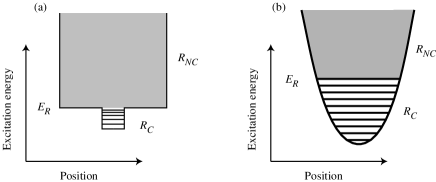
FIG. 1.: The condensate and non-condensate bands for (a) an ideal trap and (b) a harmonic trap.

FIG. 2.: Transitions in terms of quasiparticles

FIG. 3.: Condensate growth as given by the growth equation for (a) and (b) Sodium. Scattering lengths are $5.71\,{\rm nm}$ and $2.75\,{\rm nm}$, respectively.

REFERENCES

- [1] C.W. Gardiner and P. Zoller Phys. Rev. A (1997)
- [2] D. Jaksch, C.W. Gardiner and P. Zoller Phys. Rev. A (1997)
- [3] M. Anderson, J.R. Ensher, M.R. Matthews, C.E. Wieman and E.A. Cornell, Science 269, 198 (1995).
- [4] K.B. Davis, M-O.Mewes. M.R. Andrews. N.J. van Druten, D.S. Durfee, D.M. Kurn, and W. Ketterle, Phys. Rev. Lett. 75, 3969 (1995).
- [5] C.C. Bradley, C.A. Sackett, J.J. Tollet, and R. Hulet, Phys. Rev. Lett. 75, 1687 (1995).
- [6] D. J. Heinzen et al.; see http://storm.ph.utexas.edu/dept/research/heinzen/bose.html
- [7] Lene Hau et al.; see BEC HomePage,http://amo.phy.gasou.edu/bec.html/
- [8] B. Anderson and M. Kasevich; see BEC HomePage, http://amo.phy.gasou.edu/bec.html/
- [9] N.N. Bogoliubov, J.Phys. (USSR), 11, 23, (1947); reprinted in D. Pines, The Many Body Problem, Benjamin N.Y. (1962);
- [10] A. L. Fetter, Ann. Phys. (N.Y.) 70, 67, (1972); Phys. Rev. A 53, 4246 (1996)
- [11] M. Lewenstein and L. You, Phys. Rev. A 53, 909 (1996); L. You, W. Hoston, M. Lewenstein, and K. Huang, preprint; M. Lewenstein, L. You, Phys. Rev. Lett. 77, 3489, (1996)
- [12] V.L. Ginzburg and L.P. Pitaevskii, Zh. Eksp. Teor.Fiz. 34, 1240 (1958) [Sov. Phys. JETP 7, 858 (1958)]; E.P. Gross, J. Math. Phys. 4, 195 (1963); M. Edwards, R.J. Dodd, C. Clarke and K. Burnett, Journal of Research of the National Institute of Standards of Standards and Technology 101, 553, (1996); P. Ruprecht, M.J. Holland K. Burnett, and M. Edwards, Phys. Rev. A 51, 4704 (1995); M. Edwards and K. Burnett., Phys. Rev. A 51, 1382 (1995); S.A. Morgan, R. Ballagh and K. Burnett, Phys. Rev. A, to appear; M. Edwards, R. J. Dodd, C. W. Clark, P. A. Ruprecht, K. Burnett, Phys. Rev. A 53, R1950 (1996); Mark Edwards, P. A. Ruprecht, K. Burnett, R. J. Dodd, and Charles W. Clark, Phys. Rev. Lett., Phys. Rev. Lett. 77, Aug (1996); G. Baym and C.J. Pethick, Phys. Rev. Lett. 76, 6 (1996); S. Stringari, Phys. Rev. Lett. 76, 1405 (1996); S. Stringari, Phys. Rev. Lett 76,2360 (1996); L.You and M. Holland, Phys. Rev. A 53,1 (1996);
- [13] D. Jaksch, C. W. Gardiner, P. Zoller and K. Gheri, “Quantum Kinetic Theory IV; Phase diffusion in a Bose-Einstein Condensate”, In preparation
- [14] C.W. Gardiner and P. Zoller, “Quantum Kinetic Theory V; Coupled Master Equations for a Bose-Einstein Condensate Interacting with a Non-condensed Vapor”, In preparation
- [15] L.W. Nordheim, Proc. Roy. Soc. A, 119, 689 (1928); F. Bloch, Z. Phys. 52, 555, (1928); (Initial derivations of the Uehling Uhlenbeck equation); S. Kikuchi and L. Nordheim, Z. Phys. 60, 652 (1930); (More rigorous derivation of the Uehling Uhlenbeck equation); E. A. Uehling and G.E. Uhlenbeck, Phys. Rev. 43, 552 (1933) (Application of the Uehling Uhlenbeck equation to transport phenomena in quantum gases.) L. P. Kadanoff and G. Baym, Quantum statistical mechanics : Green’s function methods in equilibrium and nonequilibrium (Addison-Wesley, 1962). See also J. Ross and J.G. Kirkwood, J. Chem. Phys. 22, 1094 (1954) for a more recent derivation, and references to other contemporary work.
- [16] M. Davis, R.J. Ballagh, C.W. Gardiner and P. Zoller, “Quantum Kinetic Theory VI; The Growth of a Condensate from an Evaporatively cooled vapor.
- [17] A.A. Abrikosov, L.P. Gorkov and I.E. Dzyaloshinski, Methods of Quantum Field Theory in Statistical Physics, Dover NY (1963); E.M. Lifshitz and L.P. Pitaevskii, Statistical Physics Part 2, Landau and Lifshitz Course of Theoretical Physics Vol. 9 (Pergamon Press, Oxford 1980)
- [18] C.W. Gardiner, Phys. Rev. A 56, 1414 (1997); see also R. Dum, Y. Castin, preprint.
- [19] M. Girardeau and R. Arnowitt, Phys. Rev. 113,755 (1959)
- [20] M. Girardeau, Comment on “Particle-number-conserving Bogoliubov method which demonstrates the validity of the time dependent Gross-Pitaevskii equation for a highly condensed Bose gas”, submitted to Physical Review.
- [21] M. Lewenstein, L. You, Phys. Rev. Lett. 77, 3489, (1996)
- [22] S. Morgan, S. Choi, K. Burnett and M. Edwards, “Nonlinear Mixing of Quasiparticles in an Inhomogeneous Bose Condensate”, Oxford University preprint
- [23] J. Javanainen, Phys. Rev. A 5, 3722, (1996)
- [24] C.W. Gardiner, Handbook of Stochastic Methods, Springer (Berlin 1983, 1996)
- [25] N.G. van Kampen, Stochastic Processes in Physics and Chemistry, North Holland (Amsterdam 1982)
- [26] C.W. Gardiner, P. Zoller, R.J. Ballagh and M.J. Davis, Phys. Rev. Lett. 79, 1793 (1997).
- [27] C.W. Gardiner, Quantum Noise, Springer, (Berlin 1991)
- [28] D.F. Walls and G.J. Milburn, Quantum Optics (Springer, Berlin, 1994)
- [29] H. Haken, Laser Theory, (Springer-Verlag, Berlin, 1984)
- [30] Yu. M. Kagan, B. V. Svistunov and G.V. Shlyapnikov, Sov. Phys JETP 75, 387 (1992);Yu. Kagan and B.V. Svistunov, JETP 78, 187 (1994).
- [31] Bose-Einstein Condensation, edited by A. Griffin, D. W. Snoke, and S. Stringari (Cambridge University Press, Cambridge, 1995).
- [32] H.T.C. Stoof, Phys. Rev. Lett. 66, 3148 (1991); Phys. Rev. A 49, 3824 (1994).
- [33] D.V. Semikoz and I.I. Tkachev, Phys. Rev. Lett. 74, 3093 (1995).
- [34] J. Anglin, Phys. Rev. Lett. 79, 6 (1997)
- [35] A.J. Leggett, “Broken Gauge Symmetry in a Bose Condensate”, Article in [31]
- [36] A.J. Leggett and F. Sols, Found. Phys. 21, 353, (1984)
- [37] A. Griffin, Excitations in a Bose-Condensed Liquid, Cambridge University Press, (Cambridge 1993)
- [38] H. M. Wiseman and M. J. Collett, Phys. Lett. A 202, 246 (1995); R. J. C. Spreeuw, T. Pfau, U. Janicke, and M. Wilkens, Europhys. Lett. 32, 469 (1995); M. Olshanii, Y. Castin, and J. Dalibard, in Proceedings of the XII Conference on Lasers Spectroscopy, edited by M. Inguscio, M. Allegrini, and A. Sasso (World Scientific, Singapore, 1995); A. M. Guzmán, M. Moore and P. Meystre, Phys. Rev. A53, 977 (1996); H. M. Wiseman, A-M. Martins and D. F. Walls, Quantum Semiclassic. Opt. 8, 737 (1996); M. Holland et al., Phys. Rev. A 54, R1757 (1996); G. M. Moy, J. J. Hope, and C. M. Savage, Phys. Rev. A 55, 977 (1996); M.-O. Mewes et al., Phys. Rev. Lett. 77, 988 (1996); H. M. Wiseman, Phys. Rev. A 56, 2068 (1997)
- [39] J. Javanainen and S.M. Yoo, Phys. Rev. Lett 76, 161 (1996)
- [40] J. I. Cirac et al., Phys. Rev. A 54, R3714 (1996)
- [41] K. Molmer, Phys. Rev. A 55, 3195 (1997)
- [42] Y. Castin and J. Dalibard, Phys. Rev. A 55, 4330, (1997)
- [43] M. Abramowitz and I. Stegun, Handbook of Mathematical Functions,National Bureau of Standards, (Washington 1964)