[

Systematic Vertex Corrections through Iterative Solution of Hedin’s Equations beyond the $GW$ Approximation

Abstract

We present a general procedure for obtaining progressively more accurate functional expressions for the electron self-energy by iterative solution of Hedin’s coupled equations. The iterative process starting from Hartree theory, which gives rise to the $GW$ approximation, is continued further, and an explicit formula for the vertex function from the second full cycle is given. Calculated excitation energies for a Hubbard Hamiltonian demonstrate the convergence of the iterative process and provide further strong justification for the $GW$ approximation.

]

Much of the modern theory of many-body effects in the electronic structure of solids relies on a closed set of coupled integral equations known as Hedin’s equations [3], which connect the Green’s function $G$ of a system of interacting electrons with the self-energy operator $\Sigma$, the polarization propagator $P$, the dynamically screened Coulomb interaction $W$, and a vertex function $\Gamma$. Simultaneously solving Hedin’s equations for a specified external potential in principle yields the exact Green’s function and quasiparticle excitation spectrum without the need of actually calculating the many-electron wavefunction. Unfortunately, however, the relation between the quantities is not just purely numerical but involves nontrivial functional derivatives, so that an automated numerical solution is not feasible and approximate functional expressions with simpler dependences have to be considered instead. Most calculations of quasiparticle excitations in real materials employ the $GW$ approximation [3], which uses intermediate operators from the first cycle of an iterative solution of Hedin’s equations starting from Hartree theory as a zeroth order approximation. The $GW$ approximation neglects diagrammatic vertex corrections both in the polarization propagator and the self-energy. Its theoretical foundation lies in the assumption that sufficient convergence has been reached after the initial cycle, but rigorous evidence has so far been prevented by the inherent mathematical difficulties associated with a continuation of the iterative process. Some corroboration stems from the surprisingly good agreement with experimental spectra for a wide range of semiconductors [4, 5] and simple metals [6], while more recent studies of transition metals and their oxides highlighted deficiencies in the calculated spectra that clearly indicate a lack of convergence for materials with strong electronic correlation [7]. The $GW$ approximation has since often been reinterpreted as the first order term in an expansion of the exact self-energy in terms of the screened Coulomb interaction, and considerable effort has been spent to include second order contributions. However, such attempts have failed to produce a general improvement in numerical accuracy due to far-reaching cancellation between the additional terms [8]. In this Letter, we return to the original spirit of solving Hedin’s equations iteratively and present a scheme that generates progressively accurate functional expressions at arbitrary levels of iteration. Starting from Hartree theory, we obtain an explicit formula for the vertex function from the second iterative cycle, which mixes certain diagrams of different orders in the screened interaction. As exemplified for a Hubbard Hamiltonian, this approach indeed yields convergent excitation energies beyond the $GW$ approximation.

In our notation, the initial zeroth order self-energy and corresponding Green’s function are labelled $\Sigma^{(0)}$ and $G^{(0)}$, respectively. The sequence in which the operators are obtained during the first iterative cycle then starts with $\Gamma^{(1)}$, followed by $P^{(1)}$, $W^{(1)}$, $\Sigma^{(1)}$, and finally $G^{(1)}$. For two reasons the principal mathematical difficulty in continuing this process towards convergence lies in the calculation of the vertex function. First, it is defined only implicitly through the Bethe-Salpeter equation

$$\Gamma^{(n+1)}(1,2;3) = \delta(1,2)\delta(1,3)+\int\!\!\frac{\delta\Sigma^{(n)}(1,2)}{\delta G^{(n)}(4,5)}G^{(n)}(4,6)$$ (2)

$$\times G^{(n)}(7,5)\Gamma^{(n+1)}(6,7;3)\,d(4,5,6,7)$$

with the labels 1,2,… each denoting a set of position, time, and spin variables. While integral equations for other operators are readily solved by matrix inversion in Fourier space, the convolutions in (2) cannot easily be disentangled, so that the computational expense is prohibitive. Second, it contains the functional derivative $\delta\Sigma^{(n)}/\delta G^{(n)}$, which is nontrivial because the Green’s function $G^{(n)}$ is not explicitly contained in $\Sigma^{(n)}$ but only calculated from it by means of Dyson’s equation

$$G^{(n)}(8,9) = G^{(0)}(8,9)+\int\!\!G^{(0)}(8,1)$$ (4)

$$\times\Delta\Sigma^{(n)}(1,2)G^{(n)}(2,9)\,d(1,2),$$

where $\Delta\Sigma^{(n)}=\Sigma^{(n)}-\Sigma^{(0)}$. A numerical treatment of the vertex function becomes feasible only if the functional derivative is evaluated analytically, and if (2) can be solved explicitly for $\Gamma^{(n+1)}$. In the following we present a transformation that satisfies both requirements.

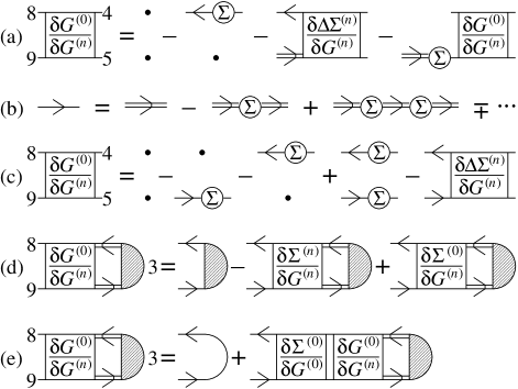
FIG. 1.: The diagrammatic series (a) for $\delta G^{(0)}/\delta G^{(n)}$ can be summed using an expansion of Dyson’s equation in the form (b) and has the explicit solution (c). By adding the first two terms on the right-hand side of (d) and applying the chain rule to the third, we obtain an integral equation (e) that can be solved by relation to the Bethe-Salpeter equation for $n=0$. Single and double line arrows indicate the Green’s functions $G^{(0)}$ and $G^{(n)}$, respectively, the encircled $\Sigma$ represents the self-energy correction $\Delta\Sigma^{(n)}=\Sigma^{(n)}-\Sigma^{(0)}$ and the shaded semicircle the vertex function $\Gamma^{(n+1)}$. Functional derivatives are labelled explicitly.

All operators relevant in this context contain as their basic building block the zeroth order Green’s function $G^{(0)}$. We therefore start by applying the chain rule

$$\frac{\delta\Sigma^{(n)}(1,2)}{\delta G^{(n)}(4,5)}=\int\!\!\frac{\delta\Sigma^{(n)}(1,2)}{\delta G^{(0)}(8,9)}\frac{\delta G^{(0)}(8,9)}{\delta G^{(n)}(4,5)}\,d(8,9).$$ (5)

The first functional derivative can in principle be evaluated at any level of iteration, so we focus on the second term. We perform the derivative of (4) with respect to $G^{(n)}$, which yields an integral equation for the four-point operator $\delta G^{(0)}/\delta G^{(n)}$ as shown in diagrammatic form in Fig. 1(a). This series can be summed using an expansion of Dyson’s equation in terms of $G^{(n)}$ with alternating signs [Fig. 1(b)]. The explicit solution is given in Fig. 1(c). Employing Dyson’s equation once more, we can write this relation more concisely as

$$\int\!\!\frac{\delta G^{(0)}(8,9)}{\delta G^{(n)}(4,5)}G^{(n)}(4,6)G^{(n)}(7,5)\,d(4,5)$$ (6)

$$= G^{(0)}(8,6)G^{(0)}(7,9)-\int\!\!G^{(0)}(8,1)G^{(0)}(2,9)$$ (8)

$$\times\frac{\delta\Delta\Sigma^{(n)}(1,2)}{\delta G^{(n)}(4,5)}G^{(n)}(4,6)G^{(n)}(7,5)\,d(1,2,4,5),$$

which still contains functional derivatives of the self-energies. Next we resubstitute $\Delta\Sigma^{(n)}=\Sigma^{(n)}-\Sigma^{(0)}$ and perform the integral with the vertex function $\Gamma^{(n+1)}$ as required by the Bethe-Salpeter equation. These two steps yield the equation shown diagrammatically in Fig. 1(d). We simplify the sum of the first two terms on the right-hand side using the relation (2) and rewrite the functional derivative in the third by applying the chain rule

$$\frac{\delta\Sigma^{(0)}(1,2)}{\delta G^{(n)}(4,5)}=\int\!\!\frac{\delta\Sigma^{(0)}(1,2)}{\delta G^{(0)}(8,9)}\frac{\delta G^{(0)}(8,9)}{\delta G^{(n)}(4,5)}\,d(8,9).$$ (9)

In this way we finally obtain the integral equation shown in Fig. 1(e), which is closely related to the Bethe-Salpeter equation for $n=0$. By comparison, we find

$$\int\!\!G^{(0)}(8,6)G^{(0)}(7,9)\Gamma^{(1)}(6,7;3)\,d(6,7)$$ (10)

$$= \int\!\!\frac{\delta G^{(0)}(8,9)}{\delta G^{(n)}(4,5)}G^{(n)}(4,6)G^{(n)}(7,5)\Gamma^{(n+1)}(6,7;3)$$ (12)

$$\times\,d(4,5,6,7).$$

We can now use this identity to sum the diagrammatic series in (2) and rewrite it in the alternative form

$$\Gamma^{(n+1)}(1,2;3) = \delta(1,2)\delta(1,3)+\int\!\!\frac{\delta\Sigma^{(n)}(1,2)}{\delta G^{(0)}(4,5)}G^{(0)}(4,6)$$ (14)

$$\times G^{(0)}(7,5)\Gamma^{(1)}(6,7;3)\,d(4,5,6,7).$$

This expression is remarkably similar to the original integral equation, except that all operators but $\Sigma^{(n)}$ on the right-hand side are replaced by their lowest order equivalents. While successive iterations dress each propagator with new sets of diagrams, the identity (10) indicates far-reaching cancellation between the expansion terms from individual propagators, yielding a much simpler expression for the vertex corrections than originally anticipated. The emergence of propagators from the lowest iterative cycle reduces the numerical expense substantially, as in practice mean-field theories are used as a zeroth order approximation. In this case $G^{(0)}$ contains no satellite spectrum but only a set of robust quasiparticle excitations. The transformation also satisfies our requirements for a numerical treatment by giving an explicit definition for the vertex function and expressing the functional derivative in a way that can be evaluated at higher orders. In the self-consistency limit $n\to\infty$, (14) implies a relation between the exact self-energy and vertex function.

In condensed matter physics, iteration conventionally starts from Hartree theory as a zeroth order approximation, so that $\Sigma^{(0)}=0$ and $G^{(0)}=G^{\rm H}$. Due to the vanishing self-energy the functional derivative in (2) is identically zero, yielding a trivial vertex function. The subsequent iteration generates the $GW$ approximation

$$P^{(1)}(1,2) = -iG^{(0)}(1,2)G^{(0)}(2,1)$$ (15)

$$W^{(1)}(1,2) = v(1,2)+\int\!\!W^{(1)}(1,3)$$ (17)

$$\times P^{(1)}(3,4)v(4,2)\,d(3,4)$$

$$\Sigma^{(1)}(1,2) = iG^{(0)}(1,2)W^{(1)}(1^{+},2),$$ (18)

where in the last equation 1⁺ implies that a positive infinitesimal is added to the time variable. $v$ is the bare Coulomb interaction. At this level the self-energy is modelled as the product of the Green’s function $G^{(0)}$ and the screened interaction $W^{(1)}$ in the random phase approximation (RPA). The functional form is reminiscent of the Fock potential, but the electronic exchange includes dynamic screening and so reaches beyond the limits of mean-field theories. Using this definition of the self-energy, it is easy to verify that its derivative with respect to the zeroth order Green’s function is given by

$$\frac{\delta\Sigma^{(1)}(1,2)}{\delta G^{(0)}(4,5)} = i\delta(1,4)\delta(2,5)W^{(1)}(1,2)$$ (21)

$$+G^{(0)}(1,2)\left[W^{(1)}(1,5)W^{(1)}(4,2)\right.$$

$$+\left.W^{(1)}(1,4)W^{(1)}(5,2)\right]G^{(0)}(5,4).$$

The corresponding vertex function $\Gamma^{(2)}$ that underlies the second iterative cycle is shown in diagrammatic form in Fig. 2. This finite set of vertex corrections is distinct from that obtained through expansion by orders of the screened interaction in that it comprises selected terms which are of zeroth, first, and second order in $W^{(1)}$.

FIG. 2.: Vertex correction $\Gamma^{(2)}$ to the $GW$ self-energy from the second iterative cycle of Hedin’s equations. Single line arrows and wiggly lines represent the zeroth order Green’s function $G^{(0)}$ and the screened Coulomb interaction $W^{(1)}$ in the random phase approximation, respectively.

Although the self-energy (18) was obtained by iteration starting from Hartree theory, in practice it is more often evaluated using a zeroth order Green’s function $G^{(0)}=G^{\rm DFT}$ from a previous density-functional calculation with $\Sigma^{(0)}=V^{\rm XC}$ equal to the exchange-correlation potential. Although this substitution violates the original spirit of the iterative scheme, physical arguments suggest only a small deviation to the propagators properly derived from density-functional theory as a zeroth order approximation [4]. Since the form of $\Sigma^{(1)}$ remains identical to that considered before, its derivative is still given by (21). The nontrivial first order vertex $\Gamma^{(1)}$ required to evaluate (14) was derived in Ref. [9] and indeed found to have insignificant numerical impact on the band gap of silicon. It is probably also negligible in the second iteration of such a calculation, so that the expression shown in Fig. 2 may still be used for $\Gamma^{(2)}$.

In the following we will supplement our discussion with the numerical investigation of a system of strongly correlated electrons that explores the effects of the vertex correction $\Gamma^{(2)}$. As the evaluation of higher order diagrams for real materials would demand computational resources beyond the scope of the present study, we consider a two-dimensional square array of 3$\times$3 atoms described by the Hubbard Hamiltonian

$${\cal H}=\sum_{{\bf R},\sigma}\epsilon_{\bf R}\hat{n}_{{\bf R}\sigma}-t\sum_{\langle{\bf R},{\bf R}^{\prime}\rangle,\sigma}c^{\dagger}_{{\bf R}\sigma}c_{{\bf R}^{\prime}\sigma}+U\sum_{\bf R}\hat{n}_{{\bf R}\uparrow}\hat{n}_{{\bf R}\downarrow}.$$ (22)

The model captures the essential physical features of materials with strong electronic correlation such as the transition metals, which are known to be inadequately described in the $GW$ approximation [7], but is simple enough to allow the calculation of full optical spectra rather than just individual matrix elements as in Refs. [8, 9]. Here, $c^{\dagger}_{{\bf R}\sigma}$ and $c_{{\bf R}\sigma}$ are the creation and annihilation operators for an electron at site ${\bf R}$ with spin $\sigma$, and we define $\hat{n}_{{\bf R}\sigma}=c^{\dagger}_{{\bf R}\sigma}c_{{\bf R}\sigma}$. The notation $\langle{\bf R},{\bf R}^{\prime}\rangle$ implies a sum over nearest neighbors only. This model was introduced in Ref. [10] to compare variations of the $GW$ approximation, and its performance within the first iterative cycle of Hedin’s equations is thus well understood. The single band of the cluster can accomodate up to 18 electrons; we consider a system of 16 electrons. The high fractional band filling resembles that of the $d$ orbitals in the late transition metals. Although we use open boundary conditions, the on-site energies $\epsilon_{\bf R}$ are chosen in such a way as to yield uniform occupation numbers in the Hartree approximation, as expected in infinite systems. For reference, the on-site energy is $2t$ for corner sites, $t$ on edge sites, and $0$ in the center of the cluster. We use medium interaction $U=4t$ and set $t=1$.

In Fig. 3 we compare the exact screened interaction $W$ with its RPA counterpart from the first iteration of Hedin’s equations, in which the polarization propagator takes the form (15), and with the second iteration. Here

$$P^{(2)}(1,2)=-i\int\!\!G^{(1)}(2,3)G^{(1)}(4,2)\Gamma^{(2)}(3,4;1)\,d(3,4).$$ (23)

As in Ref. [10], $G^{(1)}$ was obtained from a shifted zeroth order Green’s function in order to avoid problems with differing chemical potentials in the perturbation series. The figure shows the diagonal matrix element for the central site of the cluster, which because of the chosen geometry corresponds most closely to the screening in extended systems. Other matrix elements exhibit similar behavior, and the displayed curves are thus representative. For comparison, we also show results from an expansion of the polarization propagator beyond the RPA to first order in $W^{(1)}$. This approach is qualitatively distinct in that only the vertex function becomes dressed, while in the iterative scheme both $\Gamma$ and the internal propagators $G$ in (23) are simultaneously updated.

FIG. 3.: The exact screened interaction compared to the RPA, an expansion of the polarization to first order in $W$, and the second iteration of Hedin’s equations. The latter yields more accurate plasmon energies and a qualitatively correct satellite spectrum. Inset: The shift in plasmon energies is due to the explicit vertex function and remains when the diagrams are evaluated with $G^{(0)}$ rather than $G^{(1)}$, while the satellite peaks result from internal dressed propagators.

The exact screening is dominated by a pair of strong plasmon peaks at 3 and just under 6 eV, but three satellites at higher energy can be identified. While qualitatively acceptable, the RPA as a first approximation ignores the satellite spectrum and places the plasmons too high by about 1 eV. The latter deficiency is somewhat improved by the further expansion of the polarization propagator, but the description of the satellites remains poor and is not even qualitatively correct. This is in line with previous observations of far-reaching cancellation between the additional terms [8].

In comparison, the second iteration is more effective in shifting the plasmon energies, particularly for the lower peak, and also yields a better low-frequency limit for the static dielectric function. Furthermore, we observe the emergence of a satellite spectrum that is in good agreement with the exact curve concerning the number and position of features. Their exaggerated spectral weight can be traced to the satellites in the $GW$ Green’s function, which for this model are overestimated by a similar factor [10]. To isolate the effect of the vertex function, we have also evaluated (23) using $G^{(0)}$ rather than $G^{(1)}$. The resultant dielectric function, displayed in the inset in Fig. 3, retains the full shift in plasmon energies but no satellites, which are due to the internal dressed propagators. Incidentally, the graph also shows part of the apparent plasmon spectral weight to have moved across the real axis. This incorrect analytic structure is an unfortunate but common consequence of nontrivial vertex corrections and due to the occurrence of higher order poles in $P^{(2)}$. The same effect is well documented for the expansion in terms of the screened Coulomb interaction [11], where it is also observed in the present calculation. However, we have confirmed that the integral of the spectral function $-{\rm Im}W^{(2)}(\omega)/\pi$ over the positive half-axis is correctly greater than zero for all diagonal matrix elements, and as intervals of negative spectral weight are few and embedded between features with correct analytic behavior, they do not dominate convolutions in the later course of the iteration.

In summary, we have presented a scheme for the systematic construction of vertex corrections by iterative solution of Hedin’s coupled equations, and we have given explicit formulae for the propagators beyond the $GW$ approximation. Numerical results for a model of strongly correlated electrons indicate that this method not only yields improved excitation energies but is also more powerful than a comparable expansion by orders of the screened Coulomb interaction, in particular by generating a superior satellite spectrum. On a fundamental level, these findings provide the first direct evidence of convergence of the iterative approach and thus give further theoretical justification for the $GW$ approximation.

This work was supported by the Engineering and Physical Sciences Research Council. One of the authors (A.S.) acknowledges additional funding from the Deutscher Akademischer Austauschdienst under its HSP III scheme, the Studienstiftung des deutschen Volkes, the Gottlieb Daimler- und Karl Benz-Stiftung, and Pembroke College Cambridge.

REFERENCES

- [1] Electronic address: as10031@phy.cam.ac.uk
- [2] Electronic address: rwg3@york.ac.uk
- [3] L. Hedin, Phys. Rev. 139, A796 (1965).
- [4] M. S. Hybertsen and S. G. Louie, Phys. Rev. Lett. 55, 1418 (1985); Phys. Rev. B 34, 5390 (1986).
- [5] R. W. Godby, M. Schlüter, and L. J. Sham, Phys. Rev. Lett. 56, 2415 (1986); Phys. Rev. B 35, 4170 (1987); 37, 10 159 (1988).
- [6] J. E. Northrup, M. S. Hybertsen, and S. G. Louie, Phys. Rev. Lett. 59, 819 (1987); Phys. Rev. B 39, 8198 (1989).
- [7] F. Aryasetiawan, Phys. Rev. B 46, 13 051 (1992); Phys. Rev. Lett. 74, 3221 (1995).
- [8] P. A. Bobbert and W. van Haeringen, Phys. Rev. B 49, 10 326 (1994).
- [9] R. Del Sole, L. Reining, and R. W. Godby, Phys. Rev. B 49, 8024 (1994).
- [10] C. Verdozzi, R. W. Godby, and S. Holloway, Phys. Rev. Lett. 74, 2327 (1995).
- [11] P. Minnhagen, J. Phys. C 7, 3013 (1974); 8, 1533 (1975).