NTUA 67/97

OUTP-97-58P

cond-mat/9710288

Gauge-theory approach to planar doped antiferromagnets and external magnetic fields^†

K. Farakos

National Technical University of Athens, Physics Department, Zografou Campus GR-157 73, Athens, Greece,

and
N.E. Mavromatos^∗
University of Oxford, Department of (Theoretical) Physics, 1 Keble Road OX1 3NP, Oxford, U.K.

Abstract
A review is given of a relativistic non-Abelian gauge theory approach to the physics of spin-charge separation in doped quantum antiferromagnetic planar systems, proposed recently by the authors. Emphasis is put on the effects of constant external magnetic fields on excitations about the superconducting state in the model. The electrically-charged Dirac fermions (holons), describing excitations about specific points on the fermi surface, e.g. those corresponding to the nodes of a $d$-wave superconducting gap in high-$T_{c}$ cuprates, condense, resulting in the opening of a Kosterlitz-Thouless-like gap (KT) at such nodes. In the presence of strong external magnetic fields at the surface regions of the planar superconductor, in the direction perpendicular to the superconducting planes, these KT gaps appear to be enhanced. Our preliminary analysis, based on analytic Scwhinger-Dyson treatments, seems to indicate that for an even number of Dirac fermion species, required in our model as a result of gauging a particle-hole $SU(2)$ symmetry, Parity or Time Reversal violation does not necessarily occurs. Based on these considerations, we argue that recent experimental findings, concerning thermal conductivity plateaux of quasiparticles in planar high-$T_{c}$ cuprates in strong external magnetic fields, may indicate the presence of such KT gaps, caused by charged Dirac-fermion excitations in these materials, as suggested in the above model.

October 1997

^† Based on Invited talk by N.E.M. at the ‘5th Chia Workshop on Common Trends in Particle and Condensed Matter Physics’, Conference Center, Grand-Hotel Chia-Laguna, Chia (Sardegna), Italy, 1-11 September 1997.

^(∗) P.P.A.R.C. Advanced Fellow.

1 Introduction

Gauge symmetry breaking without an elementary Higgs particle, which proceeds via the dynamical formation of fermion condensates, has been a fascinating idea, which however had been tried rather inconclusively, so far, in attempts to understand either chiral symmetry breaking in four-dimensional QCD via a new strong interaction (technicolour) [1], or in the breaking of a local gauge symmetry through the formation of pair condensates in non-singlet channels [2]. In all such scenaria the basic idea is that there exists an energy scale at which the gauge coupling becomes strong enough so as to favour the formation of non-zero fermion condensates $<{\bar{f}}f^{\prime}>$ which are not invariant under the global or local symmetry in question. It is the purpose of this talk to point out that similar scenaria of dynamical gauge symmetry breaking in three-dimensional gauge theories [3] lead to interesting and unconventional superconducting properties of the theory after coupling to electromagnetism [4], and therefore may be of interest to condensed matter community, especially in connection with the high-temperature superconductors.

In a recent publication [5] we have argued that the doped large-$U$ Hubbard (antiferromagnetic) models possess a hidden local non-Abelian $SU(2)\times U_{S}(1)$ phase symmetry related to spin interactions. This symmetry was discovered using an appropriate ‘particle-hole symmetric formalism’ for the electron operators [6], and employing a generalised slave-fermion ansatz for spin-charge separation [7], which allows intersublattice hopping for holons, and hence spin flip . The spin-charge separation may be physically interpreted as implying an effective ‘substructure’ of the electrons due to the many body interactions in the medium. This sort of idea, originating from Anderson’s RVB theory of spinons and holons [7], was also pursued recently by Laughlin, although from a (formally at least) different perspective [9].

The effective long wavelength model of such a statistical system is remarkably similar to a three-dimensional gauge model of particle physics proposed in ref. [3] as a toy example for chiral symmetry breaking in QCD. In that work, it has been argued that dynamical generation of a fermion mass gap due to the $U_{S}(1)$ subgroup of $SU(2)\times U_{S}(1)$ breaks the $SU(2)$ subgroup down to a $\sigma_{3}-U(1)$ group, where $\sigma_{3}$ is the $2\times 2$ Pauli matrix. From the particle-theory view point this is a Higgs mechanism without an elementary Higgs excitation. The analysis carries over to the condensed-matter case, if one associates the mass gap to the holon condensate [5]. The resulting effective theory of the light degrees of freedom is then similar to the continuum limit of [4] describing unconventional parity-conserving superconductivity. Parity conservation is a result of the existence of an even number of fermion species, due to the underlying $SU(2)$ particle-hole spin symmetry [5, 4]. Energetics in such systems prevent the dynamical generation of a parity violating gap [10, 11].

The effect of external magnetic fields on the state of the condensate is of extreme interest, in view of recent experiments with high-$T_{c}$ cuprates pertaining to the thermal conductivity of quasiparticle (QP) excitations in the superconducting state [12]. QP thermal conductivity plateaux in a high-magnetic-field phase of these materials indicate [12] the opening of a gap for strong magnetic fields, depending on the intensity of the external field, when the latter is applied perpendicularly to the cuprate planes. As we shall argue in this talk, the phenomenon appears to be generic for systems of charged Dirac fermions in external magnetic fields, in the sense that strong enough magnetic fields are capable of inducing spontaneous formation of neutral condensates, whose magnitude scales with the magnetic field strength [13, 14, 15]. Such gaps disappear at critical temperatures proportional to the size of the gap. Despite the time-reversal breaking by the magnetic field source, there is no evidence in such systems for parity violating gaps if there is an even number of fermionic flavours, as is the case of the model of ref. [5]. However this issue is still not quite settled, and deserves further non-perturbative studies, for reasons that we shall discuss at the end of the talk. In this latter respect we should mention the recent interpretation of refs. [16, 17] about the experimental findings of ref. [12]. According to those scenaria, the high-magnetic field phase of the cuprates, is characterized by a transition of the superconducting state to a parity- and time-reversal- broken state, proposed by Laughlin some time ago [18]. In view of the results presented here, however, we shall argue that this appears not to be necessarily the case in the presence of an even number of fermion species, as in the model of ref. [5, 4]. This would allow a smooth connection of the high-magnetic-field phase gap with the zero-field superconducting gap of the model of ref. [4, 5].

It is important to notice that the experimenal indication on the opening of a gap in ref. [12] at the nodes of the $d$-wave superconducting gap, at least in the high-magnetic field phase, will be argued to imply an experimental test of the model proposed in ref. [4] and [5], involving Dirac fermions to describe excitations about specific points, such as the gap nodes, of the fermi surface of doped $t-j$ models. This is due to the fact that Dirac fermion condensation can be triggered by strong magnetic fields [13], in a Scwhinger-Dyson treatment of the relativistic field theory proposed in ref. [5], and in ref. [4]. Such a gap reduces to the superconducting gap of ref. [4] in the limit of vanishing external fields, provided that the gap-inducing statistical gauge interactions (due to the spin-spin interactions of the holons) is strong enough. A rather preliminary account of these considerations will be given below. More detailed investigations will be the subject of forthcoming work [19]. The important point in the opening of this gap is that due to the planar character of the holon excitations in these model, the opening of a gap, in the absence of a magnetic field, occurs in the Kosterlitz-Thouless mode [20, 4], i.e. occurs without implying the existence of a local order parameter, as a result of strong phase fluctuations. Hence the $d$-wave character of the superconducting state is preserved at the nodes, despite the opening of the gap there. Unfortunately at present, as far as we understand, the experiments cannot reach the weak (vanishing) magnetic field region, which could be a good testing ground for the above ideas.

2 Low-Energy Limit of Doped Planar Antiferromagnets about specific points on the Fermi Surface

We would like to start our discussion by considering the low-energy limit of doped antiferromagnetic planar systems with specific points on their fermi surface (e.g. nodes, or points where a d-wave gap vanishes, etc). Such systems might be of relevance to the physics of high-temperature superconductors, since recently it is believed that high-temperature superconductivity in cuprates is highly anisotropic and the gap symmetry is $d$-wave [21], with the gap vanishing along lines of nodes on the Fermi surface.

We shall be very brief in our discussion here. For more details we refer the reader to ref. [5] and references therein. The model considered in [5] was the strong-U Hubbard model, describing doped antiferromegnets with the constraint of no more than one elelctron per lattice site. The key suggestion in ref. [5], which lead to the non-abelian gauge symmetry structure for the doped antiferromagnet, was the slave-fermion spin-charge separation ansatz for physical electron operators at each lattice site $i$ [5]:

$$\chi_{\alpha\beta,i}\equiv\left(\begin{array}[]{cc}c_{1}\qquad c_{2}\\ c_{2}^{\dagger}\qquad-c_{1}^{\dagger}\end{array}\right)_{i}\equiv{\widehat{\psi}}_{\alpha\gamma,i}{\widehat{z}}_{\gamma\beta,i}=\left(\begin{array}[]{cc}\psi_{1}\qquad\psi_{2}\\ -\psi_{2}^{\dagger}\qquad\psi_{1}^{\dagger}\end{array}\right)_{i}~{}\left(\begin{array}[]{cc}z_{1}\qquad-{\overline{z}}_{2}\\ z_{2}\qquad{\overline{z}}_{1}\end{array}\right)_{i}$$ (1)

where $c_{\alpha}$, $\alpha=1,2$ are electron anihilation operators, the Grassmann variables $\psi_{i}$, $i=1,2$ play the rôle of holon excitations, while the bosonic fields $z_{i},i=1,2,$ represent magnon excitations [7]. The ansatz (1) has spin-electric-charge separation, since only the fields $\psi_{i}$ carry electric charge. This ansatz characterizes the proposal of ref. [5] for the dynamics underlying doped antiferromagnets. In this context, the holon fields ${\widehat{\psi}}_{\alpha\beta}$ may be viewed as substructures of the physical electron $\chi_{\alpha\beta}$ [9], in close analogy to the ‘quarks’ of $QCD$.

As argued in ref. [5] the ansatz is characterised by the following local phase (gauge) symmetry structure:

$$G=SU(2)\times U_{S}(1)\times U_{E}(1)$$ (2)

The local SU(2) symmetry is discovered if one defines the transformation properties of the ${\widehat{z}}_{\alpha\beta}$ and ${\widehat{\psi}}^{\dagger}_{\alpha\beta}$ fields to be given by left multiplication with the $SU(2)$ matrices, and pertains to the spin degrees of freedom. The local $U_{S}(1)$ ‘statistical’ phase symmetry, which allows fractional statistics of the spin and charge excitations. This is an exclusive feature of the three dimensional geometry, and is similar in spirit to the bosonization technique of the spin-charge separation ansatz of ref. [22], and allows the alternative possibility of representing the holes as slave bosons and the spin excitations as fermions. Finally the $U_{E}(1)$ symmetry is due to the electric charge of the holons.

The pertinent long-wavelength gauge model, describing the low-energy dynamics of the large-U Hubbard antiferromagnet, in the spin-charge separation phase (1), assumes the form [5]:

$$H_{HF}=\sum_{<ij>}tr\left[(8/J)\Delta^{\dagger}_{ij}\Delta_{ji}+K(-t_{ij}(1+\sigma_{3})+\Delta_{ij}){\widehat{\psi}}_{j}V_{ji}U_{ji}{\widehat{\psi}}_{i}^{\dagger}\right]+$$ (3)

$$\sum_{<ij>}tr\left[K{\overline{\widehat{z}}}_{i}V_{ij}U_{ij}{\widehat{z}}_{j}\right]+h.c.$$

where $J$ is the Heisenberg antiferromagnetic interaction, $K$ is a normalization constant, and $\Delta_{ij}$ is a Hubbard-Stratonovich field that linearizes four-electron interaction terms in the original Hubbard model, and $U_{ij}$,$V_{ij}$ are the link variables for the $U_{S}(1)$ and $SU(2)$ groups respectively. The conventional lattice gauge theory form of the action (3) is derived upon freezing the fluctuations of the $\Delta_{ij}$ field [5], and integrating out the magnon fields, $z$, in the path integral. This latter operation yields appropriate Maxwell kinetic terms for the link variables $V_{ij}$, $U_{ij}$, in a low-energy derivative expansion  [23, 24]. On the lattice such kinetic terms are given by plaquette terms of the form [5]:

$$\sum_{p}\left[\beta_{SU(2)}(1-TrV_{p})+\beta_{U_{S}(1)}(1-TrU_{p})\right]$$ (4)

where $p$ denotes sum over plaquettes of the lattice, and $\beta_{U_{S}(1)}\equiv\beta_{1}$, $\beta_{SU(2)}\equiv\beta_{2}=4\beta_{1}$ are the dimensionless (in units of the lattice spacing) inverse square couplings of the $U_{S}(1)$ and $SU(2)$ groups, respectively [5]. The above relation between the $\beta_{i}$’s is due to the specific form of the $z$-dependent terms in (3), which results in the same induced couplings $g_{SU(2)}^{2}=g_{U_{S}(1)}^{2}$. Moreover, there is a non-trivial connection of the gauge group couplings to $K$ [5]:

$$K\propto g_{SU(2)}^{2}=g_{U_{S}(1)}^{2}\propto J\eta$$ (5)

with $\eta$ the doping concentration in the sample [5, 25]. To cast the symmetry structure in a form that is familiar to particle physicists, one may change representation of the $SU(2)$ group, and instead of working with $2\times 2$ matrices in (1), one may use a representation in which the fermionic matrices ${\widehat{\psi}}_{\alpha\beta}$ are represented as two-component (Dirac) spinors in ‘colour’ space:

$${\tilde{\Psi}}_{1,i}^{\dagger}=\left(\psi_{1}~{}~{}-\psi_{2}^{\dagger}\right)_{i},~{}~{}~{}~{}{\tilde{\Psi}}_{2,i}^{\dagger}=\left(\psi_{2}~{}~{}\psi_{1}^{\dagger}\right)_{i},~{}~{}~{}~{}~{}i={\rm Lattice~{}site}$$ (6)

In this representation the two-component spinors ${\tilde{\Psi}}$ (6) will act as Dirac spinors, and the $\gamma$-matrix (space-time) structure will be spanned by the irreducible $2\times 2$ representation. By assuming a background $U_{S}(1)$ field of flux $\pi$ per lattice plaquette [4], and considering quantum fluctuations around this background for the $U_{S}(1)$ gauge field, one can show that there is a Dirac-like structure in the fermion spectrum describing the excitation about a node in the fermi surface [26, 27, 4, 25]. This leads to a conventional Lattice gauge theory form for the effective low-enenrgy Hamilonian of the large-$U$, doped Hubbard model [5]. Remarkably, this lattice gauge theory has the same form as (8). The constant $K$ of (8) can then be identified with $K$ in (3).

In the above context, a strongly coupled $U_{S}(1)$ group can dynamically generate a mass gap in the holon spectrum [11, 4, 29, 30, 31], which breaks the $SU(2)$ local symmetry down to its Abelian subgroup generated by the $\sigma_{3}$ matrix [3, 5]. From the view point of the statistical model (3), the breaking of the $SU(2)$ symmetry down to its Abelian $\sigma_{3}$ subgroup may be interpreted as restricting the holon hopping effectively to a single sublattice, since the intrasublattice hopping is suppressed by the mass of the gauge bosons. In a low-energy effective theory of the massless degrees of freedom this reproduces the results of ref. [4, 28], derived under a large-spin approximation for the antiferromagnet, $S\rightarrow\infty$, which is not necessary in the present approach.

The (naive continuum limit of) low-energy theory about such nodes of the fermi surface of the planar antiferromegnt, then, reads:

$${\cal L}_{2}\equiv=-\frac{1}{4}(F_{\mu\nu})^{2}-\frac{1}{4}({\cal G}_{\mu\nu})^{2}+{\overline{\Psi}}D_{\mu}\gamma_{\mu}\Psi$$ (7)

where now $D_{\mu}=\partial_{\mu}-ig_{1}a_{\mu}^{S}-ig_{2}\sigma^{a}B_{a,\mu}-\frac{e}{c}A_{\mu}$, $B_{\mu}^{a}$ is the gauge potential of the local (‘spin’) $SU(2)$ group, and ${\cal G}_{\mu\nu}$ is the corresponding field strength. The fermions $\Psi$ are viewed as two-component spinors. Once we gauged the $SU(2)$ group, the colour structure is up and above the space-time Dirac structure, and in two-component notation the $SU(2)$ group is generated by the familiar $2\times 2$ Pauli matrices $\sigma^{a}$, $a=1,2,3$. In this way, the fermion condensate ${\cal A}_{3}$ can be generated dynamically by means of a strongly-coupled $U_{S}(1)$. In this context, energetics prohibits the generation of a parity-violating gauge invariant $SU(2)$ term [10], and so a parity-conserving mass term necessarily breaks [3] the $SU(2)$ group down to a $\sigma_{3}-U(1)$ sector [4], generated by the $\sigma_{3}$ Pauli matrix in two-component notation.

The above symmetry breaking patterns may be proven analytically [3] on the lattice, in the strong $U_{S}(1)$ limit, $\beta_{1}\rightarrow 0$. The lattice lagrangian, corresponding to the continuum lagrangian (7), assumes the form:

$$S=\frac{1}{2}K\sum_{i,\mu}[{\overline{\Psi}}_{i}(-\gamma_{\mu})U_{i,\mu}V_{i,\mu}\Psi_{i+\mu}+$$ (8)

$${\overline{\Psi}}_{i+\mu}(\gamma_{\mu})U^{\dagger}_{i,\mu}V^{\dagger}_{i,\mu}\Psi_{i}]$$

$$+\beta_{1}\sum_{p}(1-trU_{p})+\beta_{2}\sum_{p}(1-trV_{p})$$

where $\mu=0,1,2$, $U_{i,\mu}=exp(i\theta_{i,\mu})$ represents the statistical $U_{S}(1)$ gauge field, $V_{i,\mu}=exp(i\sigma^{a}B_{a})$ is the $SU(2)$ gauge field, The fermions $\Psi$ are taken to be two-component (Wilson) spinors, in both Dirac and colour spaces [3, 5].

In the strong-coupling limit, $\beta_{1}=0$ the field $U_{S}(1)$ field may be integrated out analytically in the path integral with the result  [3]:

$$Z=\int dVd{\overline{\Psi}}d\Psi exp(-S_{eff})$$ (9)

where

$$S_{eff}=\beta_{2}\sum_{p}(1-trV_{p})-\sum_{i,\mu}{\rm ln}I^{tr}_{0}(2\sqrt{y_{i\mu}})$$ (10)

$$y_{i\mu}=-\frac{K^{2}}{4}tr[M^{(i)}(-\gamma_{\mu})V_{i\mu}M^{(i+\mu)}(\gamma_{\mu})V_{i\mu}^{\dagger}]$$

where and

$$M^{(i)}_{ab,\alpha\beta}\equiv\Psi_{i,b,\beta}{\overline{\Psi}}_{i,a,\alpha},~{}~{}a,b={\rm colour},~{}\alpha,\beta={\rm Dirac},~{}i={\rm lattice~{}site}$$ (11)

are the meson states, and ${\rm ln}I^{tr}_{0}$ denotes the logarithm of the zeroth order Modified Bessel function [32], truncated to an order determined by the number of the Grassmann (fermionic) degrees of freedom in the problem [33]. In our case, due to the $SU(2)$ and spin quantum numbers of the lattice spinors $\Psi$, one should retain terms in $-{\rm ln}I^{tr}_{0}$ up to ${\cal O}(y^{4})$:

$$-{\rm ln}I^{tr}_{0}(2\sqrt{y_{i\mu}})=-y_{i\mu}+\frac{1}{4}y^{2}_{i\mu}-\frac{1}{9}y_{i\mu}^{3}+\frac{11}{192}y_{i\mu}^{4}$$ (12)

The above expression is an exact result, irrespectively of the magnitude of $y_{i\mu}$.

The low-energy (long-wavelength) effective action is written as a path-integral in terms of gauge and meson fields, $Z=\int[dVdM]exp(-S_{eff}+\sum_{i}tr{\rm ln}M^{(i)})$, where the meson-dependent term comes from the Jacobian in passing from fermion integrals to meson ones [33]. To identify the symmetry-breaking patterns of the gauge theory (12) one may concentrate on the lowest-order terms in $y_{i\mu}$, which will yield the gauge boson masses. Higher-order terms will describe interactions. Symmetry-breaking patterns for $SU(2)$ will emerge out of a non zero VEV for the meson matrices $M^{(i)}$. This is confirmed by a detailed analysis presented in refs. [3, 5], where we refer the interested reader.

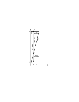
Figure 1: Phase diagram for the $SU(2)\times U_{S}(1)$ gauge theory. The critical line separates the phase of (dynamically) broken $SU(2)$ symmetry from the unbroken phase. Its shape is conjectural at this stage, in particular with respect to the order of magnitude of $\beta_{2}^{c}$. The shaded region has been analysed in ref. [3]. The dashed line represents a probable critical line in the case of the statistical model of ref. [5]. The straight line indicates the specific relation of the coupling constants in that model.

In ref. [5] a phase diagram was conjectured, which is depicted in fig. 1. The diagram indicates the existence of a ‘critical line’ in coupling constant space, seprating the phases of broken from unbroken $SU(2)$ gauge symmetry. In gauge models describing low-energy effective theories of realistic systems, the various couplings depend on the doping concentration in the sample [4], and so various regions of the phase diagram are reached by varying the doping concentration [5]. It is of interest for what follows to concentrate briefly on the line $\beta_{2}=0$ of the phase diagram. The existence of a critical $U_{S}(1)$ coupling above which dynamical mass generation for fermion occurs has been confirmed both in Scwhinger-Dyson (SD) (large flavour number $N$) [11, 4, 31] and lattice [29, 30] treatments. For instance, in large-$N$ SD treatments, the dynamically generated fermion gap in a theory with an even number of fermion flavours $N$, is parity conserving, and is given by:

$$m_{s}=\alpha{\rm exp}\left(-\frac{2\pi}{\sqrt{\frac{32}{\pi^{2}N}-1}}\right)$$ (13)

where $\alpha\equiv g_{s}^{2}/4\pi$, with $g_{s}$ the dimensionful coupling (dimensions of $\sqrt{{\rm mass}}$) of a (2+1)-dimensional gauge theory and $N$ is the number of (four-component) fermion flavours. For dynamical mass to occur $N$ must be less than $32/\pi^{2}$. For such a $N=O(1)$ (13) implies that $m_{s}<<\alpha$, and thus dynamical mass generation is an infrared (low-energy) phenomenon. For instance for $N=1$ (one four component spinor) one gets $m_{s}\simeq 0.015\alpha$.

The above analysis treated the flavour number as a fixed number. According to ref. [34], however, the non-trivial infrared dynamics of gauge theories in three dimensions induces a Wilsonian-type renormalization-group slow ‘running’ of the effective flavour number with the momentum scale. This behaviour is obtained by integrating out field modes in quantum loop diagrams with momenta below an infrared cut-off. Such a procedure, when combined with an appropriate analysis of the renormalization-improved Schwinger-Dyson equations, yields an ‘asymptotically-free’, slow running, $N(p/\alpha)$, whose increase towards low momentum scales is cut-off at a finite value $N^{*}$, at the low momentum scales $p<<\alpha$ appropriate for dynamical mass generation. It is $N^{*}$ that should enter the gap formula (13), which thus may lead to a significant increase in the gap magnitude, since $N^{*}$ is smaller than the bare $N$, which is reached only [34] for ultraviolet momentum scales $p>>\alpha$. These considerations should be born in mind when one makes attempts to connect the above results with realistic situations concerning high-temperature superconductors. For instance, the above-mentioned non-trivial infrared structure may be responsible for a non-fermi liquid behaviour of the materials in their normal phase, where no dynamical mass generation occurs [34].

At finite temperatures the gap disappears at a critical temperature $T_{c}$ which is proportional to the size of the gap at zero temperature [4]:

$$k_{B}T_{c}\simeq\frac{2}{n}m_{s}(T=0)$$ (14)

where $k_{B}$ is Boltzmann’s constant, and the number $n$ is of order ${\cal O}(6)-{\cal O}(10)$. The ambiguity in this number is due to the approximations employed in his computation. In ref. [4], where only the instantaneous approximation for the statistical SD photon propagator has been considered, $n={\cal O}(10)$. However, going beyond the instantaneous approximation reduced this number to about ${\cal O}(6)$ [35].

3 Superconducting Properties

As the next topic of our generic analysis of three-dimensional gauge models we would like to discuss the superconducting consequences of the above dynamical breaking patterns of the $SU(2)$ group. Superconductivity is obtained upon coupling the system to external elelctromagnetic potentials, which leads to the presence of an additional gauge-symmetry, $U_{E}(1)$, that of ordinary electromagnetism.

Figure 2: Anomalous one-loop Feynman matrix element, leading to a Kosterlitz-Thouless-like breaking of the electromagnetic $U_{E}(1)$ symmetry, and thus superconductivity, once a fermion mass gap opens up. The wavy line represents the $SU(2)$ gauge boson $B_{\mu}^{3}$, which remains massless, while the blob denotes an insertion of the fermion-number current $J_{\mu}={\overline{\Psi}}\gamma_{\mu}\Psi$. Continuous lines represent fermions.

Upon the opening of a mass gap in the fermion (hole) spectrum, one obtains a non-trivial result for the following Feynman matrix element: ${\cal S}^{a}=<B^{a}_{\mu}|J_{\nu}|0>,~{}a=1,2,3$, with $J_{\mu}={\overline{\Psi}}\gamma_{\mu}\Psi$, the fermion-number current. Due to the colour-group structure, only the massless $B^{3}_{\mu}$ gauge boson of the $SU(2)$ group, corresponding to the $\sigma_{3}$ generator in two-component notation, contributes to the matrix element. The non-trivial result for the matrix element ${\cal S}^{3}$ arises from an anomalous one-loop graph, depicted in figure 2, and it is given by [20, 4]:

$${\cal S}^{3}=<B^{3}_{\mu}|J_{\nu}|0>=({\rm sgn}{M})\epsilon_{\mu\nu\rho}\frac{p_{\rho}}{\sqrt{p_{0}}}$$ (15)

where $M$ is the parity-conserving fermion mass (holon condensate), generated dynamically by the $U_{S}(1)$ group. As with the other Adler-Bell-Jackiw anomalous graphs in gauge theories, the one-loop result (15) is exact and receives no contributions from higher loops [20].

This unconventional symmetry breaking (15), does not have a local order parameter [20, 4], since the latter is inflicted by strong phase fluctuations, thereby resembling the Kosterlitz-Thouless mode of symmetry breaking. The massless Gauge Boson $B_{\mu}^{3}$ of the unbroken $\sigma_{3}-U(1)$ subgroup of $SU(2)$ is responsible for the appearance of a massless pole in the electric current-current correlator [4], which is the characteristic feature of any superconducting theory. As discussed in ref. [4], all the standard properties of a superconductor, such as the Meissner effect, infinite conductivity, flux quantization, London action etc. are recovered in such a case. The field $B^{3}_{\mu}$, or rather its dual $\phi$ defined by $\partial_{\mu}\phi\equiv\epsilon_{\mu\nu\rho}\partial_{\nu}B^{3}_{\rho}$, can be identified with the Goldstone Boson of the broken $U_{em}(1)$ (electromagnetic) symmetry [4].

It is important to notice that the absense of a local order parameter of the above mechanism implies that, upon interpreting the phenomenon as being associated with the opening of a Kosterlitz-Thouless gap at the nodes of the original $d$-wave superconducting gap of the cuprate, the opening of such gap does not affect the $d$-wave nature of the state.

4 Effects of an external magnetic field

In this section we shall discuss the effects of an external magnetic field in charged excitations about the superconducting state. Due to the Meissner effect, the bulk of the superconductor is shielded off from external magnetic fields. However, in the surface region the magnetic field penetrates the superconductor. It is in such regions that the discussion below refers to.

The formalism we shall follow is essentially due to Schwinger [36], who was actually the first to compute exactly the fermion propagator in the presence of a constant external magnetic field. This formalism has been applied recently to discuss the effect of external fields in inducing fermion condensates [13, 14, 15], the latter being defined as the coincidence limit of the configuration space Dirac propagator in the presence of the external field.

The result of such analyses was that, in the context of gauge theories, like quantum electrodynamics in three and four dimensions, strong external magnetic fields are capable of inducing fermion condensates proportional to some power of the external field intensity. At finite temperatures the condensate disappears at a critical temperature proportional to the induced gap at zero temperatures. In particular, for four-dimensional QED, the gap was proportional to the square root of the magnetic field strength, and consequently the transition temperature. Such features, especially the transition temperature dependence on the gap, seem to characterize the experiment of ref. [12] on the behaviour of the thermal conductivity in the presence of magnetic fields.

What we shall argue in this section is that, if we apply the above formalism to the model of ref. [5], a similar dependence on the magnetic field strength in the high-field phase is obtained for the induced dynamical gap. What is important to notice is that in that model the gap seems to be enhanced by the presence of the strong magnetic field, given that the same set of Schwinger-Dyson equations, used to study the dynamical opening of a gap in the absence of magnetic fields in the superconducting phase of the model of ref. [5, 4], is also used in the presence of background external fields in the surface regions of the superconductor (where the magnetic field penetrates the sample), and the limit to the vanishing field phase seems to be obtained smoothly, at least formally. There are some questions regarding the existence of a critical magnetic field which might induce a transition, but we shall discuss this point later, as at present we cannot perform complete analytic computations in the model of ref. [5, 4].

We start our discussion by presenting a general discussion on the induction of a Dirac fermion condensate in three-dimensional systems in the presence of magnetic fields. The magnetic field can always be considered as truly four dimensional [4], but the charged Dirac fermions (holons) will be considered as genuinely three dimensional. When we discuss dynamical opening of a mass gap, the three-dimensional Schwinger-Dyson equations will be obtained by naive dimensional reduction of four-dimensional ones.

Let one consider a system of an even number of Dirac fermions (like the one considered in the previous section (7) in the presence of an external magnetic field $B$. For the time being we assume that we are already in the superconducting phase of the model, due to the statistical $U_{S}(1)$ interactions, which implies that the fermions acquire a parity conserving mass $+m,-m$ in two-component notation. Our point is to examine the effect of the externally applied magnetic field. This means that from now on we may ignore the statistical interactions in the model (7), and replace the effective action with that of two species of (2+1)-dimensional free Dirac fermions $\Psi_{1,2}$ in the presence of an external gauge potential

$$A_{\mu}^{ext}=-Bx_{2}\delta_{\mu 1}$$ (16)

The Lagrangian is:

$$L=\frac{1}{2}{\overline{\Psi}}(i\gamma^{\mu}(\partial_{\mu}-ieA_{\mu}^{ext})-m)\Psi$$ (17)

where $m$ is a parity conserving bare fermion mass, and the $\gamma$-matrices belong to the reducible $4\times 4$ representation, appropriate for an even number of fermion species formalism [11, 4, 5].

This problem has been studied in ref. [13], and below we sketch the derivation for the benefit of the non-expert readers. The induced fermion condensate is given by the coincidence limit of the fermion propagator

$$<0|{\overline{\Psi}}\Psi|0>=-Lim_{x\rightarrow y}trS(x,y)$$ (18)

$${\rm where}~{}~{}S(x,y)=<0|T{\overline{\Psi}(x)}\Psi(y)|0>$$

Following the proper time formalism of Schwinger [36], the propagator $S(x,y)$ in the presence of a constant external magnetic field can be calculated exactly [13]:

$$S(x,y)={\rm exp}\left(ie\int_{x}^{y}A^{ext}_{\mu}dz^{\mu}\right){\tilde{S}}(x-y)$$

$${\tilde{S}}(x)=\int_{0}^{\infty}\frac{ds}{8(\pi s)^{3/2}}{\rm exp}[-i\left(\frac{\pi}{4}+sm^{2}\right)]\times{\rm exp}[-\frac{i}{4s}x_{\nu}C^{\nu\mu}x_{\mu}]$$

$$\times[\left(m+\frac{1}{2s}\gamma^{\mu}C_{\mu\nu}x^{\nu}-\frac{e}{2}\gamma^{\mu}F_{\mu\nu}^{ext}x^{\nu}\right)\times\left(esB{\rm cot}(eBs)-\frac{es}{2}\gamma^{\mu}\gamma^{\nu}F_{\mu\nu}^{ext}\right)]$$ (20)

where $F_{\mu\nu}^{ext}$ is the Maxwell tensor corresponding to the external background gauge potential (16), and $C_{\mu\nu}=\eta^{\mu\nu}+([F^{ext}]^{2})^{\mu\nu}[1-eBs{\rm cot}(eBs)]/B^{2}$, and the line integral is calculated along a straight line. A useful expression, to be used in the following, is the Fourier transform in Euclidean space of ${\tilde{S}}(x-y)$, ${\tilde{S}}_{E}(k)$ [13]:

$${\tilde{S}}_{E}(k)=-i\int_{0}^{\infty}ds{\rm exp}[-s(m^{2}+k_{0}^{2}+{\underline{k}}^{2}\frac{tanh(eBs)}{eBs}]$$ (21)

$$\times\{[-k_{\mu}\gamma^{\mu}+m-i(k_{2}\gamma_{1}-k_{1}\gamma_{2})tanh(eBs)]\times[1-i\gamma_{1}\gamma_{2}tanh(eBs)]\}$$

A straightforward calculation, then, yields in (2+1)-dimensional space times the following result for the magnetic-field induced condensate in the limit where the bare mass $m\rightarrow 0$ [13]:

$$<0|{\overline{\Psi}}\Psi|0>=-\frac{i}{(2\pi)^{3}}\int d^{3}ktr{\tilde{S}}_{E}(k)$$ (22)

$$=-Lim_{\Lambda\rightarrow\infty}Lim_{m\rightarrow 0}\frac{4m}{(2\pi)^{3}}\int d^{3}k\int_{1/\Lambda^{2}}^{\infty}ds{\rm exp}[-s(m^{2}+k_{0}^{2}+{\underline{k}}^{2}\frac{tanh(eBs)}{eBs})]$$

$$=-Lim_{\Lambda\rightarrow\infty}Lim_{m\rightarrow 0}\frac{m}{2\pi^{3/2}}[\pi^{1/2}|eB|\frac{1}{m}+{\cal O}(\frac{1}{\Lambda})]=-\frac{|eB|}{2\pi}$$

thereby implying that in three dmensional gauge theories a strong magnetic field (such that $|eB|$ is much larger than any other mass scale in the problem), may induce a fermion gap. Notice an important difference from the corresponding four-dimensional problem, where the corresponding fermion condensate reads:

$$<{\overline{\Psi}}\Psi>\sim-|eB|\frac{m}{4\pi^{2}}({\rm ln}\frac{\Lambda^{2}}{m^{2}}+{\cal O}(m^{0}))\rightarrow 0,\qquad;m\rightarrow 0$$ (23)

and tend to zero as the bare mass $m\rightarrow 0$ , for a fixed (ultraviolet ) scale $\Lambda$. However, even in four-dimensional theories, quantum dynamics of the electromagnetic field may drastically change the situation if treated non-perturbatively [13, 15]. We shall come back to this point, and the comparison with the three dimensional theories, later in the section.

There is an elegant physical interpretation of this phenomenon, which is associated with the infrared physics in the presence of strong magnetic fields. According to ref. [13], the problem is connected to the energy spectrum of Dirac fermions in the presence of strong external fields. For the four component fermions the energy spectrum is given by the Landau levels:

$$E_{0}=\pm m$$ (24)

$$E_{n}=\pm\sqrt{m^{2}+2|eB|n}\qquad n\geq 1.$$

The density of states with energies $\pm m$ is $|eB|/2\pi$, whilst for $n\geq 1$ is $|eB|/\pi$, i.e. the condensate (22) equals the density of states at the lowest Landau level. More precisely, the propagator ${\tilde{S}}_{E}(k)$ can be decomposed over Landau poles [13]:

$${\tilde{S}}_{E}(k)=-i{\rm exp}\left(-\frac{{\underline{k}}_{vertical}^{2}}{|eB|}\right)\sum_{n=0}^{\infty}(-1)^{n}\frac{D_{n}}{k_{0}^{2}+m^{2}+2|eB|n}$$ (25)

$$D_{n}(eB,k)=(m-k_{0}\gamma_{0})[(1-i\gamma_{1}\gamma_{2}{\rm sgn}(eB))L_{n}^{0}(2\frac{{\underline{k}}_{vertical}^{2}}{|eB|})$$

$$-(1+i\gamma_{1}\gamma_{2}{\rm sgn}(eB))L_{n-1}^{0}(2\frac{{\underline{k}}_{vertical}^{2}}{|eB|})]$$

$$+4(k_{1}\gamma_{1}+k_{2}\gamma_{2})L_{n-1}^{1}(2\frac{{\underline{k}}_{vertical}^{2}}{|eB|})$$

where ${\underline{k}}_{vertical}$ denotes momentum components in a direction perpendicular to that of the applied field, and $L_{n}^{a}$ are Laguerre polynomials, with $L_{-n}^{a}=0,n>0$. In the limit $m<<|eB|$, the condensate appears due to the lowest Landau level:

$$<0|{\overline{\Psi}}\Psi|0>\simeq-\frac{m}{2\pi^{3}}\int d^{3}k\frac{{\rm exp}(-{\underline{k}}_{vertical}^{2}/|eB|)}{k_{0}^{2}+m^{2}}=-\frac{|eB|}{2\pi}$$ (26)

The above consideration can be made more precise to the more realistic case of the model (7), where one examines the effects of a strong external magnetic field on the dynamical mass generation for fermions due to the statistical $U_{S}(1)$ interaction. In four dimensional Abelian gauge theories, due to (23), the quantum dynamics of the Abelian gauge field is the dominant one. However, as mentioned above in three dimensions this may not be the case, since free three-dimensional fermions in an external field may condense for strong enough fields (22). In the three-dimensional case, of the model of ref. [5] then, the rôle of the bare mass $m$ in (22) may be played by the dynamically-generated mass due to the statistical $U_{S}(1)$ interactions, in which case the holons are driven to a new enhanced gap

$$m_{B}^{cl}=\sqrt{|<{\overline{\Psi}}\Psi>|}\sim\sqrt{|eB|}$$ (27)

under the influence of a strong magnetic field. We stress again that the above relation (27) is striclty valid in three dimensional gauge theories.

A finite-temperature $T$ (Matsubara) analysis can be performed by compactifying the time direction in (26), which results in a discrete spectrum for the energies $k_{0}\rightarrow\omega_{n}=2\pi(n+\frac{1}{2})T$. In the small mass $m<<\sqrt{eB}$ regime, the finite-temperature condensate becomes:

$$<0|{\overline{\Psi}}\Psi|0>_{T}\simeq-\frac{mT|eB|}{\pi}\sum_{n=-\infty}^{\infty}\frac{1}{4\pi^{2}T^{2}(n+\frac{1}{2})^{2}+m^{2}}=-\frac{|eB|}{2\pi}{\rm tanh}\frac{m}{2T}$$ (28)

thereby implying the absence of the condensate for any finite tmperature if the bare infrared cut-off mass $m\rightarrow 0$.

What we shall do next is to examine the effects of the quantum dynamics of the $U_{S}(1)$ field in the model (7) on the gap (27). We shall argue, following analyses [13, 15], that such quantum effects are capable of generating dynamically a small $m<<\sqrt{eB}$, which then leads to an enahnaced gap (28), under the influence of a strong (external) magnetic field. In this approach, the critical temperature coincides with the critical temperature at which the quantum corrections $m$ disappear.

In order to get an estimate of the quantum corrections, and their dependence on the magnetic field intensity, we shall follow a rather cavalier approach and, instead of solving a three-dimensional Schwinger-Dyson equation from first principles (see figure 3), we shall use results from corresponding treatments in four dimensions [13], and dimensionally reduce them.

Figure 3: The Schwinger-Dyson equation for the fermion self-energy. The curly line indicates the $U_{S}(1)$ statistical photon. Straight lines denote fermions in the presence of the external magnetic field. Blobs indicate quantum corrections (loops), which are ignored in the ladder approximation. Quantum dynamics of the electromagnetic field has been suppressed.

In three dimensions the rôle of the quantum fluctuations of the $U_{S}(1)$ gauge field becomes non-trivial due to the non-trivial infrared physics [34] (as compared to the momentum scale $\sqrt{|eB}|$). For simplicity below we shall concentrate on the area of the phase diagram of fig. 1 where the $SU(2)$ coupling constant vanishes, $\beta_{2}\rightarrow\infty$, since its presence will not alter qualitatively the results. Dynamical mass generation in the presence of an external field, due to quantum dynamics for the gauge field, has been studied in four-dimensional models in refs. [13, 15]. For our condensed-matter related problem we shall assume that the electromagnetic field is genuinly four-dimensional projected on the Cu-O planes [4]. This implies that the three-dimensional gauge theory (7) may be viewed as being obtained by appropriate dimensional reduction of a four-dimensional theory. We shall implement dimensional reduction at the level of the non-perturbative gap equations that describe dynamical mass generation, in order to study the effects of the quantum dynamics of the statistical gauge field $U_{S}(1)$ on the mass gap (27).

There are two equivalent formalisms one can follow in studies of dynamical mass generation, that of Bethe-Salpeter equation [13], and that of Scwhinger-Dyson equations [15]. Both make use of the expression (25) for the fermion propagator in external fields. The statistical $U_{S}(1)$ gauge interactions in the model (7) can be treated as usual, either in large-N expansions [11, 4] or in the weak coupling regime by summing up ladder graphs.

In the following we shall be interested in the regime where the three-dimensional coupling constant $\alpha=g_{s}^{2}/4\pi$ of the $U_{S}(1)$ interactions in the model (7), which has dimensions of mass in (2+1)-dimensions, is much weaker than $\sqrt{|eB|}$:

$$\alpha\equiv g_{s}^{2}/4\pi<<|eB|^{1/2}$$ (29)

Note that in the limit of the external field $B\rightarrow 0$, a situation which is met in the bulk of a superconductor due to the Meissner effect, the dynamical mass generation due to the $U_{S}(1)$ interactions is an infrared phenomenon, which occurs only for coupling constants relatively strong as compared to the dynamically generated mass [11] (c.f. (13)). What we shall show below is that in the presence of a strong external magnetic field, there is an enhancement of this dynamical mass in such a way that the mass in the high-field phase, the dynamically generated fermion mass $m_{B}$ is much bigger than $m_{s}$:

$$m_{s}<<\alpha=g_{s}^{2}/4\pi<<m_{B}<<|eB|^{1/2}$$ (30)

From the point of view of a strong field, then, this implies that the statistical coupling may be relatively weak, but still dynamical generation occurs, i.e. the strong magnetic field catalyses chiral symmetry breaking [13]. From our three-dimensional point of view this mass $m_{B}$ should be viewed as a quantum correction to the magnetically-induced mass gap $m_{B}^{cl}$ (27). Below we shall verify, as a consistency check of the approach, that $m_{B}^{cl}>>m_{B}$.

To get a qualitative (preliminary) description of the above phenomenon we shall dimensionally reduce the gap equations of refs. [13, 15] . The gap equations are derived for relatively weak couplings (strong magnetic fields), so that only the lowest Landau level pole enters the expression (25) for the fermion propagator ${\tilde{S}}_{E}(k)$. Adopting easily the situation of ref. [13, 15] to our case of the model (7) one gets, in the strong-field limit, the pertinent gap equation after dimensional reduction to (2+1)-dimensions .

The fact that chiral symmetry breaking is catalyzed in that work by strong magnetic fields for momentum scales $p\leq m_{B}<<\sqrt{|eB|}$, implies that the ladder approximation for the gauge bosons may prove sufficient at scales $p\geq\alpha$, since the $U(1)$ interactions appear relatively weak at such scales. This is also a valid assumption for the model (7), due to (30). In this respect, it should be pointed out that the running of the effective flavour number in three dimensions, discussed in ref. [34], also supports the above point of view, due to the asymptotic freedom (with increasing momentum scales) of the effective coupling $e_{s}^{2}=N^{-1}(p)\alpha$ of the statistical $U_{S}(1)$ interactions in the model. Moreover, the quenched approximation for fermions will also be assumed, which from our point of view will be sufficient to yield an estimate of the corrections to (27) due to the quantum dynamics of the $U_{S}(1)$ gauge field.

With these in mind, a straightforward analysis, based on that of ref. [13, 15] extended easily to the case of the model (7), yields the following expression for the dimensionally-reduced gap equation:

$$1\simeq\frac{\alpha}{\pi}\int_{-\infty}^{+\infty}\frac{dk}{k^{2}+m_{B}^{2}}\int_{0}^{\infty}dx{\rm exp}\left(-\lambda^{2}x/2\right)\frac{1}{k^{2}+x}$$ (31)

where $\lambda=|eB|^{-1/2}$ is the magnetic length, and $m_{B}$ is the dynamically generated (parity-conserving ) gap in two dimensions, obtained by dimensional reduction of the four-dimensional gap equation. In the above expression $\alpha\propto g_{s}^{2}$ is the dimensionful (dimensions of mass) fine structure constant of the statistical $U_{S}(1)$ interactions of the (2+1)-dimensional model (7), which is assumed to satisfy (30). The case $\lambda<<1$ can be studied analytically by approximating the gap equation (31) as follows:

$$m_{B}=2\alpha\int_{0}^{\infty}dx\frac{e^{-x^{2}}}{\frac{m_{B}}{\sqrt{2|eB|}}+x}\sim 2\alpha{\rm ln}[\frac{\sqrt{2|eB|}}{m_{B}}]\qquad m_{B}<<\sqrt{|eB|}$$ (32)

which results in the following $\sqrt{B}$-dependent gap in the high-field phase:

$$m_{B}\simeq\delta\sqrt{|2eB|}{\rm exp}[-\frac{m_{B}}{2\alpha}]$$ (33)

where $\delta={\cal O}(1)$. This result is in agreement with our initial assumption (30), thereby verifying the consistency of the approach. A more accurate analysis involves a numerical evaluation of the integral of the right-hand-side of the relation (31). Defining dimensionless variables $M\equiv m_{B}/\alpha$, $K\equiv\sqrt{2|eB|}/\alpha$, one obtains a set of data points from the numerical evaluation of the integral (31), which then is fitted by the approximate function for large $K>>M>1$:

$$m_{B}/\alpha=C{\rm ln}[\sqrt{2|eB|}/2\alpha]$$ (34)

The data and the fitting curve are presented in figure 4. From this one finds $C\simeq 1.42$.

Figure 4: Graphic solution of (31). Data points and fitting curve of the form (34). The fit indicates the value $C\simeq 1.42$.

It is understood that the analysis above, should be combined, for weak $\alpha$, with the result (27). So, qualitatively, the effects of an external magnetic field at zero temperature may be summarized by the enhancement of the fermion mass gap in the form:

$$m_{B}^{tot}=m_{B}^{cl}+m_{B}\sim\sqrt{\frac{|2eB|}{4\pi}}+1.42\alpha{\rm ln}[\sqrt{2|eB|}/2\alpha]$$ (35)

To get a rough estimate of the critical temperature at which the quantum corrections $m_{B}$, and according to our previous discussion the induced gap itself (28), disappear, it suffices to concentrate on the finite-temperature formalism of the above-described dynamically-generated gap due to the $U_{S}(1)$ interactions. A finite-temperature $T\neq 0$ (Matsubara) analysis of the Schwinger-Dyson equation may be performed by dimensional reduction of the corresponding four-dimensional finite-temperature gap equation obtained by Gusynin and Shovkovy in ref. [13]. The finite-temperature mass gap $m_{B}(T)$ satisfies the equation (in units where $k_{B}=1$):

$$1=2\alpha T\sum_{n=-\infty}^{+\infty}\int_{0}^{\infty}dxe^{-\lambda^{2}x/2}\frac{1}{\omega_{n}^{2}+m^{2}_{B}(T)}\frac{1}{(\omega_{n}-\omega_{0})^{2}+x}$$ (36)

where $\omega_{n}=2\pi(n+\frac{1}{2})T$. Due to thermal fluctuations the induced gap disappears at a critical temperature $T_{c}$, $m_{B}(T_{c})=0$. We are interested in determining a relation between $T_{c}$ and the externally applied magnetic field.

Figure 5: Numerical evaluation of the ingtegral (37), which determines $n^{\prime}$ in (39). Two curves are shown, corresponding to two different values of the lower limit of the integral. For the lower curve, corresponding to the value $y_{min}=0.001$ for the infrared cut-off, the fit indicates the average value $n^{\prime}\simeq 0.65$.

The critical temperature $T_{c}$ is determined by the gap equation (36), by setting $m(T_{c})=0$ and performing the summation over the frequencies. After appropriate rescaling of the integration variables, the result is:

$$1=\frac{\alpha}{2\pi T_{c}}\int_{0}^{\infty}dy{\rm exp}[-\frac{(2\pi T_{c})^{2}}{2|eB|}y]\frac{1}{(\frac{1}{4}+y)^{2}}[\pi(\frac{1}{4}+y)+coth(\pi\sqrt{y})\frac{\frac{1}{4}-y}{\sqrt{y}}]$$ (37)

Assuming $T_{c}<<\sqrt{2|eB|}$, one observes that the integrand is heavily damped for $x>2|eB|/(2\pi T_{c})^{2}$, so that the integration is effectively cut-off from above at $x\simeq 2|eB|/(2\pi T_{c})^{2}$. The dominant contributions to the integrand of (37) come from the $coth(\pi\sqrt{y})$-dependent term in the infrared regime, $y\rightarrow 0$, and are of logarithmic divergent type. A physical way of regulating such divergences is by cutting off the $\left([{\rm momentum}/2\pi T_{c}]^{2}\equiv y\right)$-integration in the infrared region by  $y_{min}=(\alpha/(2\pi T_{c}))^{2}<<1$ we can estimate the result of the integration to be:

$$\frac{2\pi T_{c}}{\alpha}\simeq C^{\prime}{\rm ln}\left(\frac{\sqrt{2|eB|}}{\alpha}\right)\qquad;\qquad C^{\prime}={\cal O}[1]$$ (38)

which is a consistent solution of the mass gap equation under the approximations we have made. In a more accurate treatment, the integral (37) can be performed numerically and is depicted in figure 5, notice that $t\equiv 2\pi T_{c}/\alpha$ and $K\equiv\sqrt{2|eB|}/\alpha$. For the lower curve, corresponding to the value $y_{min}=0.001$ for the infrared cut-off, we can deduce, from figure 5, that $C^{\prime}\simeq 5.1$. Then, from (34),(38), the following ‘empirical’ relation emerges (in units where $k_{B}=1$):

$$T_{c}\simeq n^{\prime}m_{B}(T=0)\qquad m_{B}=E(T=0)/2,~{}\alpha<<\sqrt{|eB|}$$ (39)

with $n^{\prime}\simeq 0.65$, and $E(T=0)$ the energy gap at $T=0$.

5 Conclusions and Outlook: preliminary comparison with Experiment

Some ‘phenomenology’ will help us understand better the physics involved in the above phenomenon. First we note that, due to the relativistic nature of the holon excitations about the nodes of the d-wave gap [4, 5], there is an ‘effective velocity of light’ in the problem, which coincides with the Fermi velocity for holes $v_{F}\sim 5\times 10^{-4}c$. Above we have worked in units of $\hbar v_{F}=1$, so the electric charge, $e$, is actually $e/c$, where $e$ is the physical electron charge, and $c$ is the light velocity. The magnetic length of the problem is therefore $(eB/c)^{-1/2}$ in units of $\hbar v_{F}$ or $ev_{F}B/\hbar v_{F}c=eB/\hbar c$ in SI units. This implies that the expressions for the gap should be multiplied by a factor $\hbar v_{F}\sim 5\times 10^{-4}$, in order to be expressed in $eV$. This will be understood in what follows.

Let us first remark that for magnetic field of order ${\cal O}(1)-{\cal O}(10)$ Tesla, which is the order of magnitude used in the experiment of ref. [12], and it is below the critical field that destroys superconductivity in the materials, the classical dynamics of the external electromagnetic field seems to indicate the formation of a gap (27) of order:

$$m_{B}^{cl}\sim 0.5\times\times 11.44\sqrt{|B|/10^{4}~{}{\rm Gauss}}~{}{\rm meV} \sim 18~{}{\rm meV}\qquad B=10~{}{\rm Tesla}$$ (40)

$$\sim 5.8~{}{\rm meV}\qquad B=1~{}{\rm Tesla}$$

Let us next estimate the size of the corrections, $m_{B}$, due to the quantum dynamics of the $U_{S}(1)$ field. In the model of ref. [5] the $U_{S}(1)$ coupling, $g_{s}$, is supposed to be of the same order as the $SU(2)$ coupling which is due to the effective spin-spin interactions of the Heisenberg antiferromagnetic exchange, $J$. A reasonable estimate will be therefore to take the fine structure constant of the $U_{S}(1)$ interactions, $\alpha=g_{s}^{2}/4\pi\hbar v_{F}$ of order $\eta J\simeq 0.01{\rm eV}$, for a typical (maximum) value of the doping concentration $\eta\sim 10\%$, which gives an upper bound on $\alpha\sim{\cal O}[10]{\em meV}$. In the absence of an external magnetic field, this coupling is relatively strong for $N=1$ four-component spinors to produce a superconducting gap (13) of order $0.15$ meV. This gap occurs at the nodes of the $d$-wave gap and the absence of a local order parameter [4], as reviewed in section 3, preserves the $d$-wave superconducting state. With a small gap of this size, the finite temperature analysis (14) indicates a transition temperature to a non-superconducting state of $T_{c}\simeq{\cal O}(0.1K)$, so this gap (at the nodes of the $d$-wave gap) would have disappeared at much lower temperatures, than the standard $T_{c}\simeq 100K$ of the high-$T_{c}$ cuprates. However, as mentioned previously, the effective non-trivial running [34] number entering the gap formula (13) may lead to a siginificant enhancement of the superconducting gap, and therefore of the respective critical temperature.

The phenomenon (34), discussed above, implies an enhancement of the gap by external magnetic fields in (surface) regions of the superconductor, where the external magnetic field can penetrate due to the Meissner effect. For instance, for magnetic fields of order ${\cal O}[10]$ Tesla the gap may be enhanced up to: $m_{B}(B=10~{}{\rm Tesla})\simeq 0.35\alpha\simeq 3.5meV$, which is smaller than the classical result (27), thereby justifying, to some extent, the ladder approximation, and the smallness of the quantum corrections assumed in the above calculations. This leads to a transition temperature (39) of ${\cal O}(30)$ K.

It is understood that such numbers should only be viewed as indicative, since technically the above analysis is valid only for magnetic fields $B\rightarrow\infty$. More elaborate, analytic or lattice, treatments are therefore necessary before definite conclusions are reached. Moreover, due to the Meissner effect the magnetic field is not uniformly distributed in space, something which according to the above analysis might lead to spatial anisotropies of the proposed gap $m_{B}$. The above estimates, however, appear to be reasonable enough to encourage further studies.

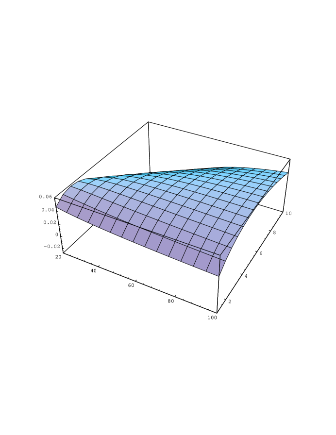
Figure 6: 3D Plot of $\frac{\alpha}{2\pi}{\rm ln}[\sqrt{2x}/\alpha]/\sqrt{2x}$. versus $(x,\alpha)$. The front horizontal axis denotes $x$. For the value of $\alpha=5$ the ratio remains almost fixed at $\sim 0.06$ (variation less than $5\%$ ), over the range of $x\sim 40-100$.

Let us now compare the above-described situation with the pertinent experimental results of ref. [12], so as to get a better feeling on the physical meaning of the above results. In that work the authors find that, for strong enough magnetic fields of ${\cal O}[1]-{\cal O}[10]$ Tesla, there are plateaux in the thermal conductivity of quasiparticle excitations about the $d$-wave state (in particular about the nodes of the d-wave superconducting gap). Such plateux are interpeted as an indication of the opening of a new gap, induced by the magnetic fields at the nodes. The authors find that the plateaux disappear at a critical temperature that depends on the magnetic field intensity, and in particular they report the empirical relation:

$$T^{exp}_{c}\propto\sqrt{|eB|}$$ (41)

for the dependence of the observed critical temperature with the external magnetic field strength. Such a dependence is not obtained in our treatment of three-dimensional relativistic fermions in a strong external magnetic field. In our analysis above, the result (38) for the critical temperature in the model of [5] was mainly due to the quantum dynamics of the $U_{S}(1)$ gauge field, and exhibits only a logarithmic dependence on the magnetic field strength. Notice that in four space-time dimensions the analogous relation indeed exhibits a $\sqrt{B}$ dependence [13]

$$T_{c}^{(4)}\sim\sqrt{|eB|}{\rm exp}[-\sqrt{\frac{\pi}{\alpha^{(4)}}}]\sim n^{\prime\prime}m_{B}^{(4)}(T=0)$$ (42)

where $n^{\prime\prime}\sim{\cal O}[1]$, $m_{B}(T=0)$ is the zero-temperature induced gap in (3+1) dimensions, and $\alpha^{(4)}$ is the four-dimensional Q.E.D. fine-structure constant, which, unlike three dimensions, is dimensionless.

From this, one would be tempted to conclude that the charged quasiparticle excitations that play a role in the phenomenon of [12] might be genuinely four-dimensional. However, due to the small value of the $Q.E.D.$ fine-structure constant $\alpha^{(4)}=1/137$ in four dimensions, the result (42) would lead to unobservably small $T_{c}$. Does this, therefore, mean, that our model of relativistic three-dimensional fermions fails completely the experimental results of [12]?

We shall argue below that the answer to this question is no, at least for the time being. Indeed, by carefully looking at the experimental data, we observe  that for the range of the magnetic field intensitites in the experiments of ref. [12] the available data cannot exclude the presence of Dirac fermions (holons) about the nodes of the d-wave gap, predicted by the model of [5], which lead to a condensate (34) with a logarithmic dependence on the magnetic field. This is mainly due to the fact that in this model one has an extra dimensionful scale $\alpha$, which may be viewed as an adjustable phenomenological parameter at this stage. For the regime of parameters relevant to the experimental data of [12], in particular for magnetic fields of order $B=1-10~{}{\rm Tesla}$, the functions $\frac{\alpha}{2\pi}{\rm ln}(\sqrt{2|eB|}/\alpha)$ and $\sqrt{2|eB|}$, which determine the critical temperature in (38) and (41), respectively, exhibit similar variations with the magnetic field $B$, provided that $\alpha\sim 5~{}{\rm meV}$. Indeed, as can be easily deduced by plotting their ratio (figure 6), for $\alpha={\cal O}(5)$ meV and $\hbar v_{F}11.55\sqrt{eB}$ of order ${\cal O}(\sqrt{40})-{\cal O}(\sqrt{400})$ meV, i.e. $B={\cal O}(1)-{\cal O}(10)$ Tesla, one finds that $\frac{\alpha}{2\pi}{\rm ln}(\sqrt{2|eB|}/\alpha)\simeq 0.06\sqrt{2eB}$ (in units of $\hbar v_{F}=1$ with $\alpha$, $\sqrt{|eB|}$, expressed in meV), with deviation of order $5-10\%$. This means that, without significant error, one can express the critical temperature (38) in the model of ref. [5] for the magnetically-induced condensate also in the form (41), with

$$T_{c}\simeq 0.9\hbar v_{F}\sqrt{|eB|}=0.45\sqrt{|eB|}~{}{\rm meV},\quad B={\cal O}(1)-{\cal O}(10)~{}{\rm Tesla},\quad\alpha={\cal O}(5)~{}{\rm meV}$$ (43)

ranging from $5.4$ K for $B\sim 1$ Tesla, to $17.4$ K for $B\sim 10$ Tesla. Such values are in agreement with the experimental findings of [12] for the above range of the magnetic fields. Notice also that the value of $\alpha\sim 5$ meV, for which the above analysis is valid, is in agreement with the generic features (5) of the model of ref. [5], and also with the Schwinger-Dyson (preliminary) analysis made above, as it is smaller than the magnetic length $\sqrt{2|eB|}$. Thus, one may fit most of the available experimental data on $T_{c}$ using our relation (38). We consider this as evidence in favour of the relevance of our gauge model to the physics of high-temperature superconductivity. It is the low-magnetic-field regime, where at present there are not many data, which may lead to decisive conclusions about the validity of our model. Note, however, that in the low-magnetic field case the above preliminary analysis is not valid, and one has to resort to lattice simulations. This is in progress [19].

We next remark that, in our analysis above, the third dimension has been ignored completely. In realistic models, the layer structure of the materials could be mimicked by viewing the system periodic along the third spatial dimension, with period equal to the interlayer distance, estimated to be of order $100$ Angstrom in the high-temperature cuprates. Formally, this would imply a Fourier series expansion of the corresponding (four-dimensional) gap equations along the third direction. This might yield (c.f. (42)) a $\sqrt{B}$ dependence for the induced gap [13], even for the quantum corrections to (27), and hence one could recover (41). However, any conclusions would be premature at this stage.

It is clear from the above discussion that a complete analysis of the three dimensional systems, both analytic (Schwinger-Dyson) and via lattice simulations, is required before any definite conclusions are drawn. Although there are encouraging preliminary results, however, many issues, like the behaviour of the system under weak magnetic fields, the connection with the zero-field case, the very existence of a critical field (phase transition), below which the gap is purely due to the $U_{S}(1)$ statistical interactions for strong coupling, etc., still remain unanswered. The study of such effects requires detailed analyses and proper lattice simulations, which are in progress [19]. Moreover, more input from experiment, such as data on the gap at the low-magnetic-field (or even zero-field ) phase, is required to provide sufficient tests of the predictions made by the model of ref. [5] in connection with the above issues.

Nevertheless, what becomes an important lesson from the above, admittedly crude, analysis is the fact that in the above model for high-$T_{c}$ dynamics there is an even number of fermion flavours [5, 4], and hence the induced self-consistent gap for those fermions, which opens up as a result of the influence of the strong external magnetic field, is not necessarily parity violating. A parity conserving, self-consistent, solution to the induced gap equation (38) has been found. However, at this stage, we are not in a definite position to exclude the possibility that a strong magnetic field induces a parity and time-reversal violating mass gap. This is the scenario suggested in ref. [17], as a possible explanation of the experimental results of ref. [12]. The presence of the external magnetic field is definitely an external source, violating time-reversal symmetry (and parity), and it is known that such sources may induce parity violating condensates in certain cases, provided they are strong enough [37]. Therefore, although in the above scenario we have found no evidence for such a phenomenon, however, a complete analysis at an effective potential level, including parity-violating dynamical condensates, along the lines of ref. [11, 10], is still lacking. This will be the topic of future work [19].

Acknowledgements

N.E.M would like to thank the organisers of the 5th Chia Workshop on Common Trends in Condensed Matter and Particle Physics, for the invitation, and for providing a thought-stimulating atmosphere during the meeting. He would also like to thank R.B. Laughlin, for explaining his ideas on a possible interpretation of the results of ref. [12] in terms of a magnetically-induced transition to a Parity- and Time-Reversal- violating ground state. The authors would like to thank I. Aitchison, B. Georgalas, G. Koutsoumbas, G. Semenoff and P. Wiegmann for discussions, and the CERN Theory division for hospitality during the last stages of this work. K.F. wishes to acknowledge partial financial support from PENED 95 Program, No. 1170, of the Greek General Secretariat of Research and Technology.

Note Added

• A. We would like to point out that an independent study of $QED_{3}$ in external magnetic fields has been made by Shpagin [38], who has performed a Schwinger-Dyson zero-temperature analysis including loops. For large magnetic fields, our analysis, based on dimensional reduction of a ladder four-dimensional theory, agrees essentially with his, as far as the logarithmic dependence of the dynamical mass $m_{B}$ on the magnetic field is concerned. From his precise analysis, however,one can also get information on subleading corrections to $m_{B}$ of the form

  $$-\alpha\left(\frac{1}{1+{\cal O}(\alpha/\sqrt{eB})}\left(1-\frac{1}{{\cal O}[{\rm ln}(\sqrt{eB}/\alpha)]}\right){\rm ln}[{\rm ln}(\sqrt{eB}/\alpha)]\right)$$

  Notice also that, as shown in ref. [38], the photon vacuum polarization is suppressed for strong magnetic fields by terms $\alpha/\sqrt{eB}$, thereby justifying the ladder approximation used in our qualitative analysis in this work. We thank V. Gusynin and V. Miransky for pointing out this reference to us, and for a useful discussion.

• B. An important aspect of the superconducting model of ref. [5], described above, was the appearance of a second superconducting phase, due to the opening of a gap at the nodes of a $d$-wave gap. This gap was caused by two species of relativistic fermions, which acquired dynamically a parity-conserving mass (13), disappearing at a temperature (14). Due to the relativistic nature of the problem this gap is of $s$-wave type. As discussed in section 5, for values of the dimensionful coupling constant $\alpha\sim{\cal O}(10)$ meV, consistent with the microscopic scenario [5] for magnetic superconductivity of the model (7), one obtains a transition temperature of order of a few hundreds of mK, which leads to a second superconducting phase. This phase appears to be in addition to the d-wave high-$T_{c}$ superconductivity, with $T_{c}={\cal O}(100)$ K, which is due to the bulk of the fermi surface for holons in the model.

  This result, which, from the point of view of the present work, pertains to the zero (or weak) external magnetic field case, may be related to the recent experimental findings of ref. [39]. These authors report on a low-temperature superconducting phase in Ni-doped BiSrCaCuO high-temperature cuprate, with $T_{c}\simeq 200$ mK. Note that the standard (d-wave) high-$T_{c}$ superconducting phase for this material has $T_{c}\simeq 77$ K. This second superconducting phase is discovered by looking at the thermal conductivity of quasiparticles, as in the experiment of ref. [12] , and was related in [39] to the opening of a gap at the nodes of the $d$-wave gap. The fact that the transition is observed after doping with Ni magnetic impurities may be suggestive of the fact that a small magnetic field is responsible for triggering the phenomenon, which from our point of view here would be similar to the magnetic catalysis phenomenon of chiral symmetry breaking, discussed above. In the paper of ref. [39] a suggestion was made, following ref. [17], that this transition signals time-reversal breaking by the condensate, which, under the influence of the magnetic field, changes its state from the one described by an order parameter $d$ to that described by a complex Time-reversal violating order parameter $d+id$. An experimental signature of such a state would be edge currents [17, 40].

  However, as we mentioned in the text, time-reversal violation may not be necessary to explain the phenomenon. Indeed, the presence of magnetic impurities in Ni-doped BiSrCaCuO may admit an alternative interpretation, which matches our theoretical analysis in section 2, namely, such impurities provide an environment that results in a strong magnetic pairing attraction among the (relativistic) fermion (holon) excitations at the nodes [5, 4]. This is supported by the fact that the order of magnitude of the transition (14) agrees with the order of magnitude observed in ref. [39]. Of course, above a critical Ni-doping concentration, supoerconductivity will be destroyed, a feature which also seems to characterise the model fo ref. [5].

  In either case, the result is the opening of a small $s$-wave Kosterlitz- Thouless (KT) gap at the nodes of the $d$-wave gap. A strong external magnetic field, then, may enhance this gap, as explained above, without inducing parity or time-reversal violation. Moreover, the smooth character of the specific-heat curves, measured in the experiment of [39] in connection with the order of the second phase transition, calls for comparison with the Kosterlitz-Thouless nature of the superconducting gap in the model of refs. [5, 4]. It will be interesting to explore further the rôle of relativistic fermion superconductivity, and the effect of magnetic fields in the context of our microscopic statistical models [5], by computing the thermal conductivity of quasiparticles, and discussing the rôle of magnetic impurities, vortices etc in such a context. These will be left for future work.

References

- [1] S. Weinberg, Phys. Rev. D13 (1976), 974; ibid D19 (1979), 1277; L. Susskind, Phys. Rev. D20 (1979), 2619.
- [2] S. Raby, S. Dimopoulos and L. Susskind, Nucl. Phys. B169 (1980), 373.
- [3] K. Farakos, G. Koutsoumbas and G. Zoupanos, Phys. Lett. B249 (1990), 101.
- [4] N. Dorey and N. E. Mavromatos, Phys. Lett. B250 (1990), 107; Nucl. Phys. B386 (1992), 614; For a comprehensive review of this approach see: N. Mavromatos, Nucl. Phys. B (Proc. Suppl.) 33C (1993), 145.
- [5] K. Farakos and N.E. Mavromatos, preprint OUTP-96-65P, NTUA-57/96, cond-mat/9611072, to appear in Phys. Rev. B; preprint OUTP-97-36P, NTUA-65/97, hep-lat/9707027, to appear in Mod. Phys. Lett. A.
- [6] I. Affleck, Z. Zou, T. Hsu and P.W. Anderson, Phys. Rev. B39 (1989), 11538.
- [7] P. W. Anderson, Science 235 (1987), 1196.
- [8] P.B. Wiegmann, Progr. Theor. Phys. Suppl. 107 (1992), 243; X.G. Wen and P.A. Lee, Phys. Rev. Lett. 76 (1996), 503.
- [9] R.B. Laughlin, Proc. 4th Chia meeting on Common Trends in Condensed Matter and Particle Physics, Chia-Laguna (Italy), September 1994.
- [10] C. Vafa and E. Witten, Comm. Math. Phys. 95 (1984), 257.
- [11] R. D. Pisarski, Phys. Rev. D29 (1984), 2423; T. W. Appelquist, M. Bowick, D. Karabali and L. C. R. Wijewardhana, Phys. Rev. D33 (1986), 3704. T. W. Appelquist, D. Nash and L. C. R. Wijewardhana, Phys. Rev. Lett. 60 (1988), 2575.
- [12] K. Krishana et. al., Science 277 (1997), 83.
- [13] V.P. Gusynin, V.A. Miransky and I.A. Shovkovy, Phys. Rev. D52 (1995), 4718; Nucl. Phys. B462 (1996), 249; V.P. Gusynin and I.A. Shovkovy, Phys. Rev. D56 (1997), 5156; V.P. Gusynin, hep-ph/9709339.
- [14] D.K. Hong, Y. Kim and S-J. Sin, Phys. Rev. D 54 (1996), 7879.
- [15] D-S. Lee, C.N. Leung and Y.J. Ng, Phys. Rev. D55 (1997), 6504.
- [16] P.W. Anderson and F.D.M. Haldane, as quoted in ref. [12].
- [17] R.B. Laughlin, preprint cond-mat/9709004, also talk at this meeting.
- [18] R.B. Laughlin, Physica C 234 (1994), 280.
- [19] K. Farakos, G. Koutsoumbas and N.E. Mavromatos, in preparation.
- [20] A. Kovner and B. Rosenstein, Phys. Rev. B42 (1990), 4748; the absence of a local order parameter in the gauge symmetry breaking patterns of (2+1)-dimensional QED is reminiscent of, although not identical to, the ‘topological order/disorder transition’ in planar systems proposed by J. Kosterlitz and D. Thouless, J. Phys. C6 (1973), 1181.
- [21] C.C. Tsuei et al., Phys. Rev. Lett. 73 (1994), 593; K.A. Moler et al., Phys. Rev. Lett. 73 (1994), 2744; D.A. Bonn et al., ibid. 68 (1992), 2390.
- [22] J. Froehlich and P. Marchetti, Phys. Rev. B46 (1992), 6535; J. Froehlich, T. Kerler and and P. Marchetti, Nucl. Phys. B374 (1992), 511.
- [23] I. J. R. Aitchison and N. E. Mavromatos, Phys. Rev. B39 (1989), 6544.
- [24] A. M. Polyakov, ‘Gauge Fields and Strings’ (Harwood 1987); S. Deser and A. N. Redlich, Phys. Rev. Lett. 61 (1989), 1541.
- [25] N. Dorey and N. E. Mavromatos, Phys. Rev. B44 (1991), 5286.
- [26] C. Burden and A.N. Burkitt, Europhys. Lett. 3 (1987), 545.
- [27] I. Affleck and J. B. Marston, Phys. Rev. B39 (1988), 3774; ibid. B39 (1989), 11538.
- [28] R. Shankar, Phys. Rev. Lett. 63 (1989), 203; Nucl. Phys. B330 (1990), 433.
- [29] E. Dagotto, A. Kocic and J.B. Kogut, Phys. Rev. Lett. 62 (1989), 1083; Nucl. Phys. B334 (1990), 279.
- [30] K. Farakos and G. Koutsoumbas, Phys. Lett. B178 (1986), 260.
- [31] P. Maris, Phys. Rev. D54 (1996), 4049.
- [32] M. Abramowitz and I. Stegun, Handbook of Mathematical Functions (Dover Publications, New York 1965).
- [33] N. Kawamoto and J. Smit, Nucl. Phys. B192 (1981), 100; I. Montvay and G. Münster, Quantum Fields on a Lattice (Cambridge Monographs on Mathematical Physics, 1994).
- [34] I.J.R. Aitchison and N.E. Mavromatos, Phys. Rev. B53 (1996), 9321; G. Amelino-Camelia, I.J.R. Aitchison, M. Klein-Kreisler, N.E. Mavromatos and D. Mc. Neill, Phys. Rev. B56 (1997), in press; I.J.R. Aitchsion, N.E. Mavromatos and D. Mc. Neill, Phys. Lett. B402 (1997), 154.
- [35] I.J.R. Aitchison, Z. Phys. C67 (1995), 303; D. Lee, Oxford U. preprint OUTP-56-P (1997), to appear.
- [36] J. Schwinger, Phys. Rev. 82 (1951), 664.
- [37] J. Ambjorn, K. Farakos and M. Shaposhnikov, Nucl. Phys. B393 (1993), 633.
- [38] A.V. Shpagin, preprint hep-ph/9611412.
- [39] R. Movshovich et al., preprint cond-mat/9709061.
- [40] G.E. Volovik, preprint cond-mat/9709084.