Abstract

By exact computer enumeration and combinatorial methods, we have calculated the designability of proteins in a simple lattice H-P model for the protein folding problem. We show that if the strength of the non-additive part of the interaction potential becomes larger than a critical value, the degree of designability of structures will depend on the parameters of potential. We also show that the existence of a unique ground state is highly sensitive to mutation in certain sites.
PACS: 82.20.Wt, 36.20.-r, 36.20.Ey, 82.20.Db.

I. Introduction

Biologically active proteins fold into a native compact structure despite the huge number of possible configurations [1]. Though the mechanism of protein folding is not fully understood, it has been known since the re-folding experiments of Anfinsen [2] that globular proteins fold in the absence of any catalytic biomolecules. From this fact, it has been established that for proteins,the three dimensional folded structure is the minimum free energy structure, and, the information coded in the amino-acid sequence is sufficient to determine the native structure [3]. The compactness of this unique native state is largely due to the existence of an optimal amount of hydrophobic amino-acid residues [4], since these biological objects are usually designed to work in water [5]. The relation between the primary one dimensional sequence and the final compact three dimensional structure is the task of the protein folding problem.

In addition to the paradoxical problem of kinetics and time scales of the folding process [6], there is another mystery. If proteins are made randomly by amino acids, the number of all possible such proteins with typical length of $100$, is far larger than the number of proteins which actually occur in nature. One hypothesis is that the naturally selected sequences are special because they are coded for structures that have unique and stable native states, allowing for easy folding. Thus a central question of protein evolution is how mutational change in the amino acid sequence leads to changes in the structure and stability.

Some efforts have been made in order to study the stability of proteins against mutation by searching the two dimensional configuration space [7, 8]. One simple model used in these studies is the H-P model [9]. In this model there are only two types of chain monomers, hydrophobic (H) and polar (P). Every H-H contact between topological neighbours is assigned a negative contact energy, and other contact interactions are set to zero.

Recently Li et al. [10], have looked at this problem in three dimensions. Calculating the energy of all possible 27-mers in all compact three dimensional configuration, they have found that, there are a few structures, into which a high number of sequences uniquely fold. This structures were named ”highly designable” and the number of sequences which fold into each state was named its ”designability”. In their H-P model, they choose the contact energy between H and P monomers by some physical arguments [10, 11]. Other significant points of their work are: a) Only a few percent of sequences have unique ground state; b) There is a jump in energy gap for these highly designable structures. Thus the highly designable structures are more stable against mutation and thermal fluctuation.

Dill and Chan [12] have argued that many of the phenomena observed in proteins can be adequately understood in terms of the H-P model, but according to the work of Pande et al. [13] the designability of a conformation does depend on the nature of interactions between monomers. May be any interaction leads to some highly designable structures, but different interactions yield different patterns.

In our work we study this problem for an additive potential. We will show that there are some highly designable structures for this potential, but the low designable structures will disappear because of degeneracy of ground state. We will show that there is a ladder structure for energy levels for this form of potential. We then add a non-additive part to the energy, then the ground state degeneracy of low designable structures will be removed. We show there is a critical value for non-additive part of potential, where below this critical value the patterns of highly designable structures are fixed, but above this critical value the designability of structures is sensitive to the value of non-additive part of the potential. We show that the sequences which fold to highly designable structure are sensitive to mutation of some sites.

An additive potential has the following advantages:

a) It allows us to prepare a very fast algorithm which is then possible to run on a PC.

b) It enables us to solve and study some parts of the problem by combinatorial methods.

c) It gives a clear picture for designability.

d) A ladder spectrum for the energy levels results, thus it arms us to study the problem for non-additive potentials.

II. The Model

We consider an H-P lattice model [9]. In this model only non-sequential nearest neighbours interact. Because the native structures of proteins are compact with the H type monomers sitting in the core, the effective potentials which are usually used, all of the forces are attractive (negative values for potential) and the strength of the force between H-H monomers is greater than others. We can write the general form of the potential in an arbitrary energy scale as:

$$E_{\bf PP}=0,\hskip 28.45274ptE_{\bf HP}=-1,\hskip 28.45274ptE_{\bf HH}=-2-\gamma.$$ (1)

The most usual choice of H-P model potential corresponds to the limit $\gamma\gg 1$ [7, 8, 9, 12], however physical arguments are consistent with a smaller value for $\gamma$, for instance $\gamma=0.3$ was used by Li et al. [10]. They have calculated the energy of all of $2^{27}$ sequences in $103,346$ compact configuration for a $27$-sites cube, by a huge enumeration.

In the case $\gamma=0$, we have an additive potential. If we let ${\bf H}=-1$, and ${\bf P}=0$, we can rewrite the potential in the form,

$$E_{\sigma_{i}\sigma_{j}}=\sigma_{i}+\sigma_{j}.$$ (2)

Following Li et al. [10], we consider only compact structures of sequences with length 27, occupying all sites of a $3\times 3\times 3$ cube [14]. There are $103,346$ compact configurations which are not related to each other by rotation and reflection symmetries. Let us call the set of all compact structures, the structure space.

A protein of length $N$ may be shown by an $N$-component vector

$$|\sigma\rangle=|\sigma_{i_{1}},\sigma_{i_{2}},\dots,\sigma_{i_{N}}\rangle,$$ (3)

where $i_{n}=1,2$ refers to P and H residues. Thus the number of such $N$-component vectors for proteins with length $27$ is $2^{27}$. Let us call the set of $|\sigma\rangle$, the sequence space.

Because of the additive form of the potential, we can write the energy of a given $|\sigma\rangle$ in any spatial configuration as,

$$E=\sum_{i=1}^{27}p_{i}\sigma_{i},$$ (4)

where $p_{i}$’s are the number of non-sequential neighbours of the $i$th monomer, or by introducing the neighbourhood vector $|P\rangle$,

$$E=\langle\sigma|P\rangle.$$ (5)

The vector $|P\rangle$ has 27 components and at $i$th component has the number of neighbours of the $i$th monomer. Due to the shape of $|P\rangle$ the type of neighbours is not relevant and all we have to do is count the non-sequential neighbours. This gives us an additional symmetry for the energy that is different from spatial symmetries. For example any of the sites in a two dimensional $5\times 5$ square for two spatial configurations which are shown in figs. 1a and 1b, have equal neighbours, but the labels of their neighbours are not the same. Visualisation of the same effect in 3 dimensions is a bit harder, but it dose exist.

The space of all $3$ dimensional structures has $103,347$ members for all compact full filled structures in a $3\times 3\times 3$ cube. Due to this additional symmetry this space is divided into $6291$ subspaces, where all members of each subspace have the same $|P\rangle$. Let the number of members of a subspace be, $N_{d}$. The range of $N_{d}$ is from $1$ to $96$. Fig. 2, shows that the frequency of large values of $N_{d}$, is low. Interestingly there are a lot of $|P\rangle$’s which only point to one structure.

FIG. 1.: The number of neighbours for corresponding sites in these two configuration are the same, but the neighbours are not, for instance, site 18 in (a) is the neighbour of 5, but they are not adjacent in (b).

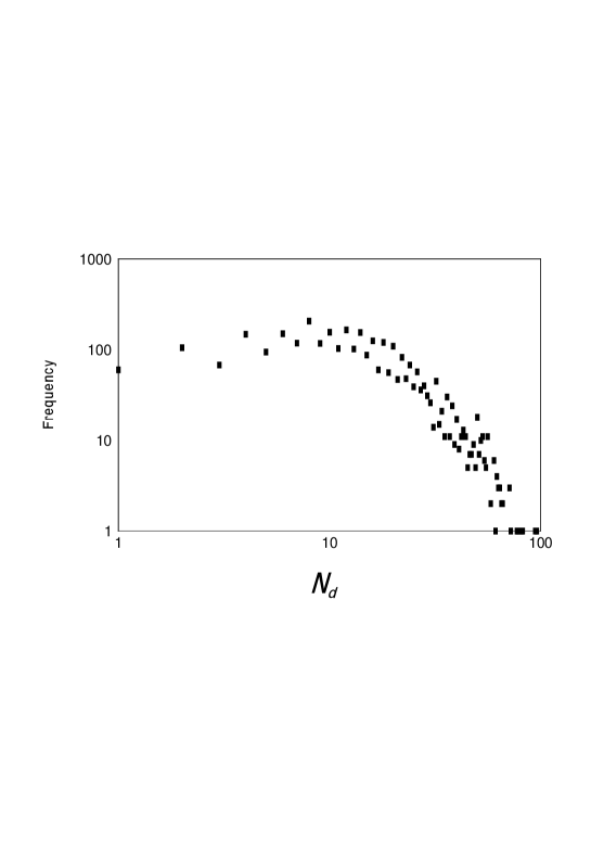
FIG. 2.: Histogram of $N_{d}$ for members of structure space. It is interesting that there are some $P$ sets with $N_{d}=1$.

We have calculated the energy of all $2^{27}$ $|\sigma\rangle$ on all $|P\rangle$. We find the degeneracy of ground state in structure space. One can see the distribution of number of ground state degeneracies $g$, for all of $2^{27}$ sequences in fig. 3. There are only a few sequences which have non-degenerate ground state, this corresponds to the $8.47\%$ of sequences at $g=1$. If energy of one sequence is minimised in a $|P\rangle$ with $N_{d}$ greater than one it has degenerate ground state. According to definition of designability, such sequences should not be considered. The distribution of $N_{s}$ is presented for $\gamma=0$ in fig. 4. Comparing this figure with fig. 2 of Li et al. [10], we observe that there is no similarity. This suggests that designability ($N_{s}$), is sensitive to the value of $\gamma$, which is $\gamma=0$ in our work, whereas Li et al. chose $\gamma=0.3$. However as we shall see later, the fact that at $\gamma=0$, we have an additive potential plays an important role. In fact a small value of $\gamma$ radically change the picture.

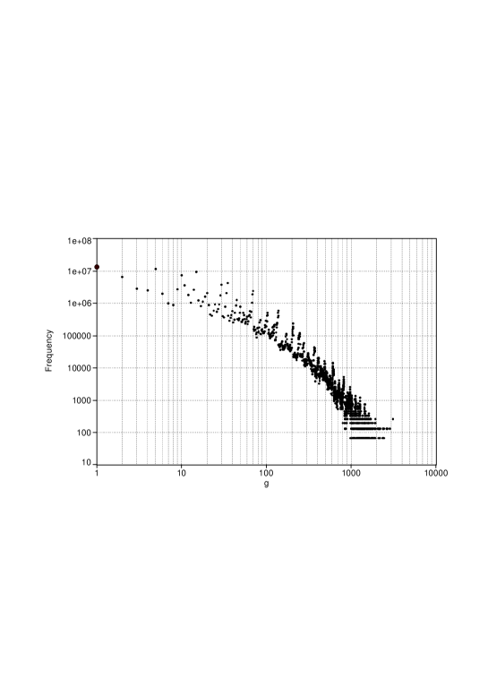
FIG. 3.: Histogram of degeneracy of ground state. The sequences which have non-degenerate ground state, correspond only to $g=1$, in this diagram.

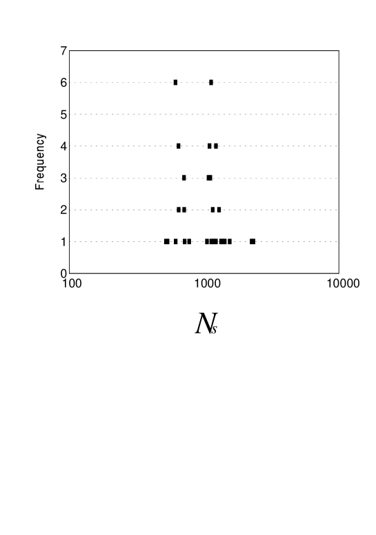
FIG. 4.: Histogram of $N_{s}$ for additive potential.

If we consider all of sequences which have non-degenerate ground state in structure space, we get a new picture for designability. This means that we calculate the designability of all $|P\rangle$’s, and not only those with $N_{d}=1$. This is contrast to $N_{s}$ which had only $N_{d}=1$.

To recognise this difference, we show designability of structures, by $N^{\prime}_{s}$. Fig. 5 shows the distribution of $N^{\prime}_{s}$. Many of points in this fig. 5 are related to some $|P\rangle$’s with $N_{d}\neq 1$. We shall use this picture to express the nature of the energy gap in the case $\gamma\neq 0$ in section V.

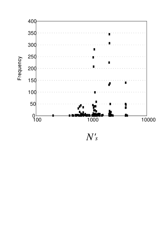
FIG. 5.: Histogram of $N_{s}^{\prime}$ for additive potential. Note that many of points in this diagram correspond to some $|P\rangle$’s which point to more than one spatial configuration.

In our enumeration we have calculated the energy of any sequence in all $6291$ $|P\rangle$’s, but in fig. 5 , we show the results for $3153$ $|P\rangle$’s which are not related to each other by reverse labelling. We can not reduce the structure space according to this symmetry before enumeration. Reverse labelling for a nonsymmetric sequence gives two different configurations which may have different energies.

III. Energy levels

The number of non-sequential neighbours is related to type of site. A $3\times 3\times 3$ cube has 8 corner sites $(C)$, 12 link sites $(L)$, 6 face sites $(F)$, and one centre site $(O)$ (fig. 6). $C$ sites have three neighbours, where two of them are connected by sequential links and there is only one non-sequential neighbour. Similarly $L$, $F$ and $O$ sites have 2, 3 and 4 non-sequential neighbours respectively. We must add 1 to these numbers for two ends of chain.

FIG. 6.: A $3\times 3\times 3$ cube has 8 corner sites, 12 link sites, 6 face sites and 1 centre site.

This sites are divided in two classes, $\{C,F\}$ and $\{L,O\}$. In a self avoiding walk in this cube, we must jump in any step from one set to other. The first set has 14 members and the second has 13. Thus a walk passes through $C$ and $F$ sites in odd steps, and through $L$ and $O$ sites in even steps. In other words, the odd components of $|P\rangle$ are 1 or 3, and even components are 2 or 4, (except the 1st and 27th components which are like even components). Thus,

$$|P\rangle=|p_{1},\dots,p_{27}\rangle,$$ (6)

where,

$$p_{i}=\left\{\begin{array}[]{llr}1,3&\ \ \ \ \ {\rm odd}&\ i^{\prime}s;\\ 2,4&\ \ \ \ \ {\rm even}&\ i^{\prime}s.\\ \end{array}\right.$$ (7)

Therefore the energy for a sequence $\sigma_{\alpha}$ in a structure $P_{\mu}$ is

$$E_{\alpha\mu} = \langle\sigma_{\alpha}|P_{\mu}\rangle$$ (8)

$$= \sum_{i\in{\rm odd}}(p_{\mu i}-1)\sigma_{\alpha i}+\sum_{i\in{\rm even}}(p_{\mu i}-2)\sigma_{\alpha i}+\sum_{i\in{\rm odd}}\sigma_{\alpha i}+2\sum_{i\in{\rm even}}\sigma_{\alpha i}.$$ (9)

By introducing the new binary variable $x$ the above can be rewritten as,

$$E_{\alpha\mu}=\sum_{i=1}^{27}2x_{\mu i}\sigma_{\alpha i}+\sum_{i\in{\rm odd}}\sigma_{\alpha i}+2\sum_{i\in{\rm even}}\sigma_{\alpha i},$$ (10)

where,

$$x_{i}=\left\{\begin{array}[]{llr}0&\ \ \ \ \ p_{i}=1\ {\rm or}\ 2;\\ 1&\ \ \ \ \ p_{i}=3\ {\rm or}\ 4.\\ \end{array}\right.$$ (11)

Two last terms in eq. (10) are independent of $|X\rangle$ or $|P\rangle$, thus they result in a constant, which can be ignored when comparing energies of a sequence in different configurations. The first term in eq. (10) is an integer times two, thus it results in a ladder energy spectrum with gaps of 2. Therefore the energy gap for all of structures is the same, and there is no difference between low designable and high designable structures.

IV. Combinatorial Approach

Our aim is to find the $N^{\prime}_{s}$ for any spatial configuration, determined by a vector $|P\rangle$. Because $|X\rangle$ has a simpler structure, than $|P\rangle$, we shall use $|X\rangle$ instead of $|P\rangle$. Any vector $|X\rangle$, has seven $1$’s and twenty $0$’s. One of the $1$’s is in the even sites, and the others are in odd sites. Energy could be calculated by performing a “logical and” of two binary numbers ($|\sigma\rangle$ and $|X\rangle$). For example, a typical $|P\rangle$ is,

To recognise odd and even components of the vectors, we show them in the above form, writing the even sites below. The vector $|X\rangle$ corresponding to the above $|P\rangle$ is,

On the other hand $|\sigma\rangle$’s have a similar form:

Where we show P monomers by numerical equivalence of them. Recall that numeric equivalence for H monomers is $-1$. Energy of any sequence in any spatial configuration is calculated by inner product of its $|\sigma\rangle$ to corresponding $|X\rangle$. For the above $|\sigma\rangle$ and $|X\rangle$ the energy is $5{\bf H}$. This value is related to exact value of energy according to eq.(10) by a factor of two and two sequence dependent additional terms, since we are interested in the ground state and the energy gap of a sequence, the sequence dependent term may be ignored, as structure determines these quantities alone.

By construction any $|X\rangle$ has six $1$’s in odd sites, and one $1$ in even sites. If we don’t consider any other constraint for $|X\rangle$, we obtain an upper limit for number of $|X\rangle$’s.

$$n={14\choose 6}\times{13\choose 1}=39039.$$ (12)

This is far larger than the number of possible $|X\rangle$’s which we have obtained by enumeration, that is $6291$. The fact that all 39039 possible configuration don’t exist points to extra constraints which are yet to be discussed. If all 39039 of $|X\rangle$’s were to exist each of them would have to be unique ground state of only one sequence, thus removing all interest! To see this, it is enough to insert an H into $|X\rangle$ where ever one finds a 1, and P for zeros. Indeed absence of some of these vectors in real world makes some of the other more preferable in nature.

The connectivity of a self avoiding walk, further constraints the $|X\rangle$. For example to pass through centre site, the walk has to pass through two face sites. This means that the only $1$ (corresponding to centre site) in even sites must be sandwiched between two $1$’s in odd sites (face sites). This constraint reduces the number of possible $|X\rangle$’s. Two $1$’s in odd sites are fixed by even $1$, and only 12 sites remain for four other $1$’s. Then there are,

$$n={12\choose 4}\times{13\choose 1}=6435,$$ (13)

vectors. This number is still larger than exact number of $|X\rangle$s by $144$. Although due to our enumeration we know these $144$ vectors, we can not find the complex constraints which prune them out, and we shall continue our calculation as though these 144 vectors were correct. Of course the values are different from exact enumeration, however it can be seen that this difference is not too large, and it may be considered as an approximation to the exact solution. Also we aid a computer enumeration including the extra 144 vectors and have compared the results with the combinatorial calculation. This has served as a check on our code.

We now proceed to calculate $N^{\prime}_{s}$ for the following example:

First let us introduce some new parameters and notations. We will show the energy of a $|\sigma\rangle$ in an $|X\rangle$ as:

$$E=E(a,b,c)=(a+b+c)H,$$ (14)

where $a,b$ and $c$ are related to energy parts which come from centre ($1$ in lower row), faces which are connected to centre, and energy of other parts, respectively. For example energy of following $|\sigma\rangle$:

in $|X_{0}\rangle$, is $E(0,2,3)=5{\bf H}$.

Besides, we name the number of pairs of $1$’s in the upper row of $|X\rangle$ as $z$ and the number of $1$’s in two ends of vectors as $y$. For $|X_{0}\rangle$, $z=2$, and $y=1$.

Now we try to count the number of all polymers which have their energy minimised in $|X_{0}\rangle$ and, there is no other $|X\rangle$ with energy equal to ground state for them. To do this we discuss all possible cases.

i: $E(1,2,4)$

Such polymers have at least seven H sites corresponding to $1$’s of $X_{0}$. These polymers have minimum possible energy, thus $X_{0}$ is a minimum energy configuration for them. But it must be checked whether it is a unique ground state or not. First consider polymers which in addition to these seven H’s have another H monomer in their upper row sites,

The energy of this sequence in following $|X\rangle$ is $7{\bf H}$ too.

Then the ground state of polymers which have additional H monomers in corresponding to upper row $0$’s of $X_{0}$, is degenerate, and they don’t count in $N^{\prime}_{s}$ of $X_{0}$. The above discussion is independent of value of $a$ and $b$ in $E(a,b,4)$, and degrees of freedom to choose sites for H monomers is limited to lower row sites.

For the $|X\rangle$ with $z\neq 1$ (like $X_{0}$) polymers can not have H monomers in the lower sites between two upper row $1$’s. For example, the following sequence,

has energy $7{\bf H}$ in following $|X\rangle$ too.

Then the contribution of polymers with $E(1,2,4)$ in $N^{\prime}_{s}$ is:

$$N^{\prime}_{s}({\bf i})=2^{12-(z-1)}=2^{13-z}$$ (15)

ii: $E(0,2,4)$

In this case if $z>1$ (such as $X_{0}$) the ground state is degenerate. It can be seen that any sequence with energy $E=(0,2,4)$ in $X_{0}$ state has the same energy in $X_{2}$ state. In the case $z=1$, only the sites in lower row by condition that they are not a neighbour of corresponding upper $1$’s of $X$, have freedom to be an H or P monomer. There are $2\times 6-z-y$ sites which don’t have this freedom in lower row. Then,

$$N^{\prime}_{s}({\bf ii})=\left\{\begin{array}[]{ll}2^{2-y}&\ \ \ \ \ z=1\\ 0&\ \ \ \ \ z>1\\ \end{array}\right.$$ (16)

iii: $E(1,0,4)$

In this case there is only one sequence with nondegenerate ground state. For our example, $X_{0}$, this sequence is,

In the above sequence changing any P monomer to H type, will cause the ground state to becomes degenerate. Then,

$$N^{\prime}_{s}({\bf iii})=1$$ (17)

iv: $E(1,1,4)$

For this case $b$ is $1$, and if this $1$ comes from right or left neighbour of lower $1$, it has different solutions. Then we introduce new parameters ($z_{R}$, $y_{R}$) and ($z_{L}$, $y_{L}$), which are similar to old $z$ and $y$, when right or left neighbour $1$ of lower $1$ will be omitted. For $X_{0}$ we have $z_{R}=0$, $z_{L}=1$ and $y_{R}=y_{L}=y=1$. By introducing this new parameters this case is very similar to case ii, and the difference comes from number of corresponding $1$’s in upper row (five instead six), and no restriction in value of $z$. Then,

$$N^{\prime}_{s}({\bf iv})=2^{3+z_{R}+y_{R}}+2^{3+z_{L}+y_{L}}.$$ (18)

v: Other cases

All of the other cases for ground state energy are degenerate, and need not be considered.

With this analysis it is possible to find $N^{\prime}_{s}$ for any $|X\rangle$. For our $X_{0}$ example it is,

$$N^{\prime}_{s}({\bf i}) = 2^{11}$$ (19)

$$N^{\prime}_{s}({\bf ii}) = 0$$ (20)

$$N^{\prime}_{s}({\bf iii}) = 1$$ (21)

$$N^{\prime}_{s}({\bf iv}) = 2^{4}+2^{5},$$ (22)

that gives,

$$N^{\prime}_{s}(X_{0})=2097$$ (23)

In this way all of the values of $N^{\prime}_{s}$’s can be calculated. Had the $144$ additional structures been taken out, the calculation of $N^{\prime}_{s}$ for the problem would correspond to enumeration exactly. However taking these structures out is too complex and would have to be done case by case. Besides of the value of $N^{\prime}_{s}$, this calculation shows that the sequences whit non-degenerate ground state have between 4 to 6 H type monomers in face sites and no one in corner sites. Indeed in our model the stability of polymers is very sensitive to mutation in corner sites.

V. Nonadditive potentials

In the case $\gamma\neq 0$ the potential is non-additive. In this case we can write the energy of $\alpha$th sequence in $\mu$th spatial configuration as:

$$E_{\alpha\mu}=\langle\sigma_{\alpha}|P_{\mu}\rangle-{\textstyle\frac{1}{2}}\gamma\langle\sigma_{\alpha}|M_{\mu}|\sigma_{\alpha}\rangle.$$ (24)

Where $\sigma$ and $P$ are the sequence and neighbourhood vectors, that introduced in previous sections. $M$ is the adjacency matrix for this configuration.

$$M_{ij}=\left\{\begin{array}[]{llr}1&\ \ \ \ \ {\rm if\ the}\ i{\rm th\ and}\ j{\rm th\ monomers\ are\ adjacent;}\\ 0&\ \ \ \ \ {\rm otherwise}.\\ \end{array}\right.$$ (25)

Any $|P\rangle$ has $N_{d}$ different $M$-matrices. The first term in eq. (24) was calculated in the case $\gamma=0$, and we need calculate only the last part. The aim of our calculation is to find the ground state. In any compact configuration in a $3\times 3\times 3$ cube, there are $28$ non-sequential neighbour pairs. Thus the contribution of the last term in energy is less than $28\gamma$. We have shown that energy spectrum for the previous case has a ladder structure with energy gap equal to $2$. In this case these split to some sublevels (fig. 7). Then if we choose $\gamma<\frac{2}{28}$ the levels are separate. Of course this is a lower estimation for $\gamma$. In the next section we will obtain a better estimate for lower and upper limits of the critical value of $\gamma$.

FIG. 7.: Energy levels of additive potential split to sublevels for non-additive potential.

From the result of the additive potential we have a subset $P$ in the space of all spatial configurations which gives the minimum energy to folding. This $P$ subset has $N_{d}$ members which all of them have the same $|P\rangle$. For small $\gamma$’s the ground state and the first excited state are between these $N_{d}$ structures, and it is not necessary to calculate the energy for all of $103,346$ spatial structures for any sequence,except for sequences which their ground state is in structures with $N_{d}=1$. For The $N_{d}=1$ structures the value of $N_{s}$ does not change, and it is not necessary to run the program. The first excited state of these sequences are in an other $P$ subset. Thus to find the energy gap for them the program must be run over all of the $103,346$ structures. We have calculated this energy spectrum, and have found the new $N_{s}$ for all $103,346$ structures. We show the results for $51,704$ configuration which are unrelated by reverse labelling symmetry in fig. 8. We have found the energy gap for first excited state for all sequences. You can see the diagram of mean of energy gap vs. $N_{s}$ in fig. 9. This figure shows that highly designable structures which are related to $P$ subsets with one member.

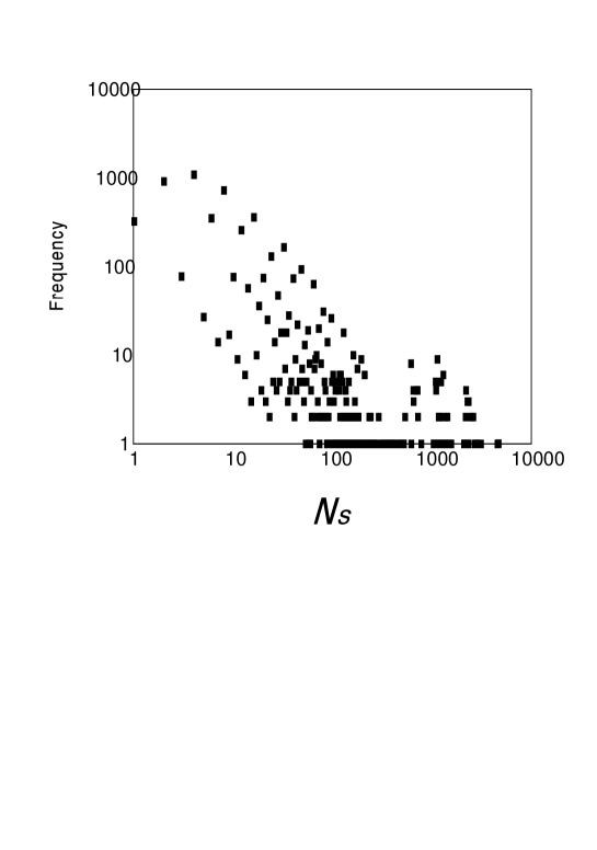
FIG. 8.: Histogram of $N_{s}$ for non-additive potential.

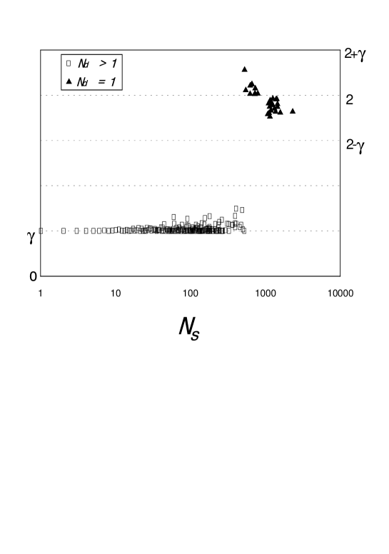
FIG. 9.: The mean of energy gap vs. $N_{s}$. There is a jump in energy gap for highly designable structures. All of these highly designable structures have $N_{d}=1$.

In this enumeration we have calculated the energy spectrum for all of the sequences which have nondegenerate ground state for the additive potential. We had removed some of the sequences because of degeneracy of ground state in additive potential case. It is possible that this degeneracy will be removed by the non-additive part of the potential, and some of the sequences have unique ground state for non-additive potential. But the energy gap for these sequences is of order of $\gamma$, and if we consider them it causes a shift in horizontal axes to bigger $N_{s}$ and bring down the points nearer to $\gamma$ value in vertical direction in fig. 9. These make this figure more similar to results of Li et al. [10]. In their work the energy gap for low designable structures are of order of $\gamma$ ( they choose $\gamma=0.3$) also.

VI. Estimation of $\gamma_{c}$

The energy levels for the additive potential have a ladder structure, as it had been proven in previous sections. The energy gaps between the levels is $2$ in our arbitrary energy unit.

In the case of $\gamma\neq 0$ the energy has two parts (eq. 24). The first part comes from additive part of potential and does not change. Second part comes from non-additive part of potential, and is equal to number of H-H non-sequential neighbours in spatial configuration. Because this non-additive part, the energy spectrum is changed, and any level is splited to some sublevels (fig. 7).

If contribution of the second part to energy is less than $2$, for all structures, the ground state and excited state of any polymer is between $|P\rangle$ partners of its ground state for additive potential , except for $|P\rangle$ with $N_{d}=1$, where there is only ground state.

Let $\delta e_{0}$ be the difference of ground state energies of additive and non-additive potentials, and $\delta e_{1}$ be difference energy of first excited state in the case of $\gamma=0$ with minimum of new energies for the sequence in the structures corresponding to these excited states (there is no uniqueness constraint for excited states). If $\delta e_{0}-\delta e_{1}<2$ the ground state doesn’t change and the values of $N_{s}$ for structures that we presented in past section don’t change. By increasing $\gamma$, the absolute values of $\delta e_{0}$ and $\delta e_{1}$ increase.

To find the difference between $\delta e_{0}$ and $\delta e_{1}$ one have to calculate the difference in H-H contacts in ground state structure and maximum of H-H contacts in excited level structures.

This difference has two sources. Because the energy levels in the case $\gamma=0$ are separated by 2, then difference of them comes from replacing a H monomer from $O$ site to an $L$ site, or from an $F$ site to a $C$ site. Both of them cause increasing in energy by 2. But it is possible that these replacing decrease the energy by $2\gamma$. For example consider one $F$ site with no H neighbour will go to one $C$ site with two non-sequential H neighbours (this monomer must be an end residue). then this gives an upper limit for $\gamma_{c}$, that is $1$.

The other source for increasing the H-H contacts, comes from replacing H monomers in $L$ and $F$ sites by the same type sites. These changes only are relevant in the case $\gamma\neq 0$. The maximum of increasing in H-H contacts because these replacing are $6\gamma$, related to the sequences which have 4 H monomers in the $F$ sites and 5 to 7 in $L$ sites in their ground state structures. Thus the lower limit for $\gamma_{c}$ is $\frac{2}{2+6}=0.25$. Therefore,

$$0.25<\gamma_{c}<1.$$ (26)

This shows that there is a non zero value for $\gamma_{c}$, which for $\gamma$ less than it, the ground state structure of sequences doesn’t change. Indeed $\gamma_{c}$ distinguishes two phases. If $\gamma<\gamma_{c}$, the degree of designability of structures is independent of $\gamma$, and the change in value of $\gamma$ only changes the energy gaps. On the other hand for $\gamma>\gamma_{c}$, the designability of structures becomes sensitive to the value of $\gamma$, and the patterns of highly designable structures will be changed if the potential changes.

If the designability is the answer of “why has the nature selected a small fraction of possible configurations for folded states?”, the above discussion shows that this selection is potential independent if $\gamma<\gamma_{c}$, and sensitive to inter monomers interactions if $\gamma>\gamma_{c}$.

Acknowledgements

We would like to thank J. Davoudi for motivating the problem, R. Golestanian and S. Saber for helpful comments, and S. Rouhani for helpful comments throughout the work and reading the manuscript.

REFERENCES

- [1] L. Stryer, Biochemistry, (W.H. Freeman and Company, San Francisco, 1988); Protein Folding, T.E. Creighton ed., (W.H. Freeman and Company, New York, 1992).
- [2] C.B. Anfinsen, E.Haber, M.sela, and F.H. White, Pros. Natl. Acad. Sci. USA 47, 1309 (1961).
- [3] C.B. Anfinsen, Science 181, 223, (1973).
- [4] K.A. Dill, S. Bromberg, K. Yue, K.M. Fiebig, D.P. Yee, P.D. Thomas, and H.S. Chan, Protein Science 4, 561 (1995).
- [5] T. Garel, H. orland, E. pitard, “Protein folding and Heteropolymers”, Spin Glasses and Random Fields, A.P. Young, ed., World scientific.
- [6] C. Levinthal, J. Chem. Phys. 65, 44 (1968).
- [7] H.F. Lau, and K.A. Dill, Pros. Natl. Acad. Sci. USA 87, 638 (1990).
- [8] H.S. Chan, K.A. Dill, J. Chem. Phys. 95, 3775 (1991).
- [9] H.S. Chan, K.A. Dill, J. Chem. Phys. 90, 492 (1989); H.S. Chan, K.A. Dill, D. Shottle, “Statistical Mechanics and Protein Folding”, Prinston Lectures on Biophysics, W. Bialek ed., (World Scientific, 1992).
- [10] H. Li, R. Helling, C. Tang, N. Wingreen , Science 273, 666 (1996).
- [11] H. Li, C. Tang, N. Wingreen , Phys. Rev. lett. 79, 765 (1997).
- [12] K.A. Dill, Biochemistry 29, 7133, (1990); H.S. Chan, and K.A. Dill , Pros. Natl. Acad. Sci. USA 87, 6388, (1990).
- [13] V.S. Pande, A.YU. Grosberg, T. Tanaka, J. Chem. Phys. 103, 9482 (1995).
- [14] E. Shakhnovich, and A. Gutin, J. Chem. Phys. 93, 5967 (1990).