Abstract

Mixed atomistic and continuum methods offer the possibility of carrying out simulations of material properties at both larger length scales and longer times than direct atomistic calculations. The quasi-continuum method links atomistic and continuum models through the device of the finite element method which permits a reduction of the full set of atomistic degrees of freedom. The present paper gives a full description of the quasicontinuum method, with special reference to the ways in which the method may be used to model crystals with more than a single grain. The formulation is validated in terms of a series of calculations on grain boundary structure and energetics. The method is then illustrated in terms of the motion of a stepped twin boundary where a critical stress for the boundary motion is calculated and nanoindentation into a solid containing a subsurface grain boundary to study the interaction of dislocations with grain boundaries.

Keywords: dislocations(A), grain boundaries(A), constitutive behaviour(B), finite elements(C)

1 Introduction

A longstanding ambition in the modeling of materials has been that of rationalizing and predicting the observed mechanical properties of materials on the basis of an understanding of their constituent defects. The advent of ever more powerful computers alternatives has ushered in the possibility of carrying out rudimentary calculations of this type directly on the basis of full atomistic simulations. However, an alternative class of models has sought to exploit atomistic insights without abandoning altogether the powerful resources that are associated with continuum theories. One such approach is the quasicontinuum method (Tadmor, Ortiz and Phillips, 1996) which links the kinematic constraints, and attendant degree of freedom reduction offered by the finite element method, to total energies predicated entirely on atomistic analysis.

The push to develop models of defect interactions has come from experimental observations on ever-smaller length scales. Recent micromechanical observations routinely explore problems in which small numbers of defects are responsible for the mechanical properties of interest (see, for example, Gerberich, Nelson, Lilleodden, Anderson and Wyrobek, 1996). The experimental advent of nanomechanics as ushered in by a host of high resolution microscopies such as high-resolution TEM and atomic scale resolution surface probes such as the STM and the AFM has led to theoretical demands as well. One of the theoretical responses to this challenge has been the attempt to build simulation tools that allow for the analysis of multiple length scales simultaneously. Before turning to the quasicontinuum method itself, we mention two examples that are antecedents to the approach advocated here.

The broad class of models known as cohesive zone models have as their aim the incorporation of constitutive nonlinearity to account either for the “core” material at a crack tip (Barenblatt 1962) or at a dislocation core (Peierls 1940). One of the significant outcomes of these calculations that is especially noteworthy for the present purpose is the fact that the incorporation of the constitutive nonlinearity introduced by the cohesive zone eliminates (or at least ameliorates) the singularities that are inherited from an analysis predicated purely on the basis of linear elasticity. A recent advance in cohesive zone technology has been the exploitation of cohesive zone elastic potentials calculated using density functional calculations (Xu, Argon and Ortiz, 1995), in the study of dislocation nucleation near a crack tip. As will be more evident below, the quasicontinuum method takes its cue from the cohesive zone approach in that it is noted that constitutive nonlinearity, especially as dictated by an underlying atomistic analysis, that gives this approach its power.

An alternative class of models that is built around the same insights as those associated with cohesive zone approaches are those that effect a linkage between two different spatial regions, one of which explicitly treats each and every atomic degree of freedom with its requisite nonlinearity and a second of which is treated either by traditional linear elasticity or its discrete analog (Kohlhoff, Gumbsch and Fischmeister (1991), Thomson, Zhou, Carlsson and Tewary (1992)). Such methods necessitate the management of boundary conditions that permit the matching of the two regions. However, the logic that stands behind such methods is nearly identical to that advocated here. The assertion is that in the immediate vicinity of the defect, it is essential to have a sufficient level of resolution as to capture the sometimes complex local atomic rearrangements that characterize them. On the other hand, the contention is that far away from the defect, there is no reason to doubt the efficacy of continuum mechanics. In their present incarnations, these mixed methods have the difficulty in that each problem must be treated on a case by case basis with the boundary between the fully atomistic region and the rest of space designed a priori. The quasicontinuum method to be described below is founded on the basis of adaptive strategies in which, in the course of the calculation, the region of full atomistic resolution can vary in response to the evolution of both loading and defects.

The present paper is written with two clear objectives. First, it is our aim to generalize the earlier statements of the quasicontinuum method so as to allow for the treatment of problems involving more than one grain. It is well known that a range of phenomenology in the mechanics of materials including Hall-Petch type phenomena, grain boundary sliding and Nabarro-Herring creep, trace their existence to the presence of grain boundaries. The formulation as described in an earlier paper (Tadmor, Ortiz and Phillips, 1996) was noncommittal with respect to the question of how one might incorporate grain boundaries as a synthetic element of the material’s microstructure and it is a key aim of the present work to remove that ambiguity.

The second objective of the present paper is to provide the logical foundation for the generalization of the method to a number of different contexts. Work to further extend the quasicontinuum method is presently in progress in a number of different areas, all of which rest upon the foundations laid here. One of the key extensions is to make the method fully three dimensional, which allows for the realistic simulation of phenomena such as dislocation junction formation and dislocation nucleation. An additional area of development concerns the need to explicitly evaluate the dynamical trajectories undertaken in a given process at finite temperature. In particular, we see the quasicontinuum method as a possible meeting point for molecular dynamics and continuum thermodynamics. Finally, to allow for the treatment of alloys and even elemental materials such as silicon, the method has required generalization to situations in which the crystallography is characterized by the presence of more than one atom per unit cell. Although these topics will not be described in the present paper explicitly, preliminary efforts have been forged in all of these directions, all of which have been built around the ideas that are set forth here.

The organization of the remainder of the paper is as follows. Section 2 presents an overview of the quasicontinuum method. The detailed description of the individual components of the methodology may be found in Section 3. This will be followed in section 4 by a discussion of validation of the method, with full atomistic calculations serving as the benchmark for success with particular reference to the use of quasicontinuum calculations for the study of grain boundary structure and energetics. Sections 5 and 6 complete the description with applications that exploit the capacity of the method to examine deformation problems involving more than a single grain.

2 Overview

In this section, we undertake a description of the quasicontinuum method, with special attention drawn to the subtleties that attended the generalization to problems involving more than one grain. As discussed in the introduction, one of the fundamental precepts around which the quasicontinuum method was built was the idea that direct atomistic simulation has both strengths and weaknesses. The clear advantage of the atomistic perspective is that such calculations are capable of providing the requisite resolution to account for the highly nonlinear and sometimes counterintuitive atomic arrangements that are found in the defect core. Indeed, it has been found that in some circumstances such atomic level details are the source of known macroscopic anomalies in the material’s behavior (Christian 1983). On the other hand, the weakness of the atomistic approach is the huge number of redundant degrees of freedom away from such defects. The quasicontinuum method attempts to incorporate both of these insights by allowing for full atomic scale resolution near defect cores while exploiting a coarser description further away.

We begin with an overview of the conceptual elements of the quasicontinuum method as described in Tadmor, Ortiz and Phillips (1996). The key idea is that of kinematic slavery in which by virtue of the finite element method (FEM), the positions of the majority of atoms are entirely constrained and determined only by the displacements of the nodes tied to the element of which they are a part. Once the geometric disposition of the body is established, the problem becomes one of determining the total energy. From a traditional continuum mechanics viewpoint, such as that offered by the linear theory of elasticity, the total energy may be computed on the basis of a phenomenological constitutive law such as Hooke’s law. The aim in Tadmor, Ortiz, Phillips (1996), by way of contrast, has been to use atomistic calculations to inform the energetic statement of the continuum mechanics variational principle. This step offers the constitutive nonlinearity alluded to above, and allows naturally for the emergence of lattice defects such as dislocations.

We now give a formal description of the formulation of the quasicontinuum method generalized to account for the presence of multiple grains, restricting attention to those problems in which the undeformed state of the body is polycrystalline. We take the view that the body whose disposition is of interest should be thought of as a collection of a possibly huge number, $N$, of atoms. In fig. 1, we show the body which is imagined to be built up of a variety of different grains with Bravais lattice vectors schematically indicated. The presence of a crystalline reference configuration is exploited in the sense that for many regions of the crystal, it is unnecessary to save lists of atomic positions since they can be generated as needed by exploiting the crystalline reference state. A given atom in the reference configuration is specified by a triplet of integers ${\bf l}=(l_{1},l_{2},l_{3})$, and the grain to which it belongs. The position of the atom in the reference configuration is then given as,

$${\bf X}(l)=\sum_{a=1}^{3}l_{a}{\bf B}_{a}^{\mu}+{\bf R}^{\mu},$$ (1)

where ${\bf B}_{a}^{\mu}$ is the $a^{\mit th}$ Bravais lattice vector associated with grain $G_{\mu}$ and ${\bf R}^{\mu}$ is the position of a reference atom in grain $G_{\mu}$ which serves as the origin for the atoms in grain $G_{\mu}$.

Once the atomic positions have been given, from the standpoint of a strictly atomistic perspective, the total energy is given by the function

$$E_{tot}=E_{exact}({\bf x}_{1},{\bf x}_{2},{\bf x}_{3},...,{\bf x}_{N})=E_{exact}(\{{\bf x}_{i}\}),$$ (2)

where ${\bf x}_{i}$ is the deformed position of atom $i$. We adopt the convention that capital letters refer to the undeformed configuration while lower case letters refer to the deformed configuration. The energy function in eq. (2) depends explicitly upon each and every microscopic degree of freedom, and as it stands becomes intractable once the number of atoms exceeds one’s current computational capacity. The problem of determining the minimum of the potential energy is in the context noted above nothing more than a statement of conventional lattice statics. We will now proceed to construct the formulation of the method in a step-by-step fashion. We begin with the introduction of kinematic constraints which have the effect of reducing the number of degrees of freedom being accounted for by selecting a small subset of $R$ atoms from the total set of $N$ atoms. These atoms serve as “representative atoms”, and remain the only unconstrained degrees of freedom in the problem. A finite element mesh with nodes corresponding to the positions of the representative atoms is then defined. By virtue of finite element interpolation we may compute the total energy from the equation given above, but now with a substantial fraction of the atoms participating geometrically as nothing more than drones since their positions are entirely determined by the displacements of the adjacent nodes. Quantitatively, if $\alpha$ is an index over the representative atoms, then the interpolated position ${\bf x}_{i}^{int}$ of any other atom $i$ may be obtained by

$${\bf x}_{i}^{int}=\sum_{\alpha}N_{\alpha}({\bf X}_{i}){\bf x}_{\alpha},$$ (3)

where $N_{\alpha}({\bf X}_{i})$ is the finite element shape function centered around the representative atom $\alpha$ (which is also a FEM node) evaluated at the undeformed position ${\bf X}_{i}$ of atom $i$. In particular, we may write the total energy as

$$E_{tot}=E_{exact}({\bf x}_{1}^{int},{\bf x}_{2}^{int},...,{\bf x}_{N}^{int})=E_{exact}(\{{\bf x}_{i}^{int}\}).$$ (4)

At this stage not much has been gained since the computation of the total energy is still predicated upon a knowledge of all of the atomic positions, though now many of the atomic positions are constrained. We now make the additional assumption that the energy may be written in a form that is additively decomposed, such that

$$E_{tot}=\sum_{i=1}^{N}E_{i},$$ (5)

which presupposes the existence of well-defined site energies $E_{i}$, and is typical in many current atomistic formulations such as the embedded-atom method (EAM). The summation runs over all atoms in the solid. Because of this, the sum written above remains intractable in the sense that if we interest ourselves in computing the total energy, we are still obliged to visit each and every atom. The spirit of the problem that we are faced with is now identical to that of numerical quadrature, and what we require at this point is a scheme for approximating the sum given above by summing only over the representative atoms with appropriate weights selected so as to account for differences in element size and environment. In particular, we desire

$$E_{tot}\approx\sum_{\alpha=1}^{R}n_{\alpha}E_{\alpha}.$$ (6)

The crucial idea embodied in this equation surrounds the selection of some set of representative atoms, each of which are intended to characterize the energetics of some spatial neighborhood within the body as indicated by the weight $n_{\alpha}$. As yet, the statement of the problem is incomplete in that we have not yet specified how to determine the summation weights, $n_{\alpha}$. We treat the problem of the determination of $n_{\alpha}$ in a manner analogous to determination of quadrature weights in the approximate computation of definite integrals. In the present context the goal is to approximate a finite sum (“definite integral” on the lattice) by an appropriately chosen quadrature rule where the quadrature points are the sites of the representative atoms. Physically the quantity $n_{\alpha}$ may be interpreted as the “number of atoms represented” by the representative atom $\alpha$. The quadrature rule (eq. (6)) is designed such that in the limit in which the finite element mesh is refined all the way down to the atomic scale (a limit we denote as fully refined) each and every atomistic degree of freedom is accounted for, and the quadrature weights are unity (each representative atom represents only itself). On the other hand, in the far field regions where the fields are slowly varying, the quadrature weights reflect the volume of space (which is now proportional to the number of atoms) that is associated with the representative atom. The details of this procedure may be found in section 3.1.

The description given above describes the essence of the formulation as it is currently practiced. We now describe an additional energetic approximation that simplifies the energy calculations and also makes it possible to formulate boundary conditions which mimic those expected in an elastic continuum. The essential idea is motivated by fig. 2, which depicts the immediate neighborhood of a dislocation core. In particular, for this Lomer dislocation we note the characteristic geometric signature of the core, namely, the pentagonal group of atoms in the core region. We now focus our attention on the environments of two of the atoms in this figure, one (labeled $A$) in the immediate core region, and the other (labeled $B$) in the far field of the defect. It is evident that the environment of atom $A$ is nonuniform, and that each of the atoms in that neighborhood experiences a distinctly different environment. By way of contrast, atom $B$ has an environment that may be thought of as emerging from a uniform deformation, and each of the atoms in its vicinity sees a nearly identical geometry.

As a result of these geometric insights, we have found it convenient to compute the energy $E_{\alpha}$ from an atomistic perspective in two different ways, depending upon the nature of the atomic environment of the representative atom $\alpha$. Far from the defect core, we exploit the fact that the atomic environments are nearly uniform by making a local calculation of the energy in which it is assumed that the state of deformation is homogeneous and can be well-characterized by the local deformation gradient ${\bf F}$. To compute the total energy of such atoms, the Bravais lattice vectors of the deformed configuration ${\bf b}_{a}$ are obtained from those in the reference configuration ${\bf B}_{a}$ via ${\bf b}_{a}={\bf F}{\bf B}_{a}$. Once the Bravais lattice vectors are specified, this reduces the computation of the energy to a standard exercise in the practice of lattice statics.

On the other hand, in regions that suffer a state of deformation that is nonuniform, such as the core region around atom $A$ in fig. 2, the energy is computed by building a crystallite that reflects the deformed neighborhood from the interpolated displacement fields. The atomic positions of each and every atom are given exclusively by ${\bf x}={\bf X}+{\bf u}({\bf X})$, where the displacement field ${\bf u}$ is determined from finite element interpolation. This ensures that a fully nonlocal atomistic calculation is performed in regions of rapidly varying ${\bf F}$. An automatic criterion for determining whether to use the local or nonlocal rule to compute a representative atom’s energy based on the variation of deformation gradient in its vicinity will be presented in section 3.2. The distinction between local and nonlocal environments has the unfortunate side effect of introducing small spurious forces we refer to as “ghost” forces at the interface between the local and nonlocal regions. A correction for this problem is also discussed in section 3.2.

Once the total energy has been computed and we have settled both the kinematic and energetic bookkeeping, we are in a position to determine the energy minimizing displacement fields. As will be discussed below, there are a number of technical issues that surround the use of either conjugate gradient or Newton-Raphson techniques. Both of these techniques are predicated upon a knowledge of various derivatives of the total energy with respect to nodal displacements and are explained in section 3.3.

As noted in the introduction, one of the design criteria in the formulation of the method was that of having an adaptive capability that allowed for the targeting of particular regions for refinement in response to the emergence of rapidly varying displacement fields. For example, when simulating nanoindentation, the indentation process leads to the nucleation and subsequent propagation of dislocations into the bulk of the crystal. To capture the presence of the slip that is tied to these dislocations, it is necessary that the slip plane be refined all the way to the atomic scale. The adaption scheme to be described in section 3.4 allows for the natural emergence of such mesh refinement as an outcome of the deformation history.

The goal of the present section has been to elucidate the key conceptual elements involved in using the quasicontinuum method. However, as was noted above, certain features in the formulation involve subtleties demanding further attention. In the following sections, we undertake a more detailed analysis of some of those issues.

3 Details of the Methodology

3.1 Reduced Atomic Representation

In this section we discuss the selection of the representative atoms, and the construction of an expression of the total energy that depends only on the degrees of freedom of the representative atoms. We consider the undeformed body to be a crystalline solid, i.e., a collection of $N$ atoms, which occupy a region $B_{0}$ and may be arranged in many grains $G_{\mu}$ (see fig. 1). The undeformed position ${\bf X}_{i}$ of any atom $i$ is obtained from the coordinate of a reference atom and an associated set of Bravais lattice vectors that are specified for each grain as discussed earlier in (eq. (1)). The deformed configuration of the body is described by a displacement function ${\bf u}$ which depends on ${\bf X}$ and the deformed position of any atom $i$ can be obtained as

$${\bf x}_{i}={\bf X}_{i}+{\bf u}_{i},$$ (7)

where ${\bf u}_{i}={\bf u}({\bf X}_{i})$.

On loading the solid, the equilibrium configuration of the body is defined by the set of displacements ${\bf u}_{i}$ which minimizes the potential energy function

$$\Pi({\bf u})=E_{tot}({\bf u}_{1},...,{\bf u}_{N})-\sum_{i=1}^{N}{\bf f}_{i}\cdot{\bf u}_{i},$$ (8)

where $E_{tot}$ is the total energy of the system obtained from an atomistic formulation, ${\bf f}_{i}$ is the external force acting on the atom $i$ and ${\bf u}$ satisfies the essential boundary conditions of the problem. This is the well-known method of lattice statics (LS). Now, as stated earlier, we assume that $E_{tot}$ can be decomposed as a sum over the energies of individual atoms $E_{i}$, i.e.,

$$E_{tot}({\bf u}_{1},...,{\bf u}_{N})=\sum_{i=1}^{N}E_{i}({\bf u}_{1},...,{\bf u}_{N}),$$ (9)

and eq. (8) becomes

$$\Pi({\bf u})=\sum_{i=1}^{N}E_{i}({\bf u}_{1},...,{\bf u}_{N})-\sum_{i=1}^{N}{\bf f}_{i}\cdot{\bf u}_{i}.$$ (10)

Many of the conventional atomistic formulations (such as the embedded-atom method) admit such a decomposition, although it is not admissible in the more sophisticated density functional approach. For example, the embedded-atom method (Daw, Baskes 1986) provides that for a homonuclear material the energy at site $i$ is given by

$$E_{i}=\frac{1}{2}\sum_{j}\phi(r_{ij})+f(\rho_{i}),$$ (11)

where $r_{ij}$ is the distance from atom $i$ to the neighbor $j$, $\phi$ is a pairwise interaction, $\rho_{i}$ is the electron density at the site $i$ and $f(\rho)$ is the embedding energy. The potentials are assumed to have a cutoff radius of $r_{\rm cut}$, i.e., any atom interacts directly only with those atoms within a distance $r_{\rm cut}$ from it.

The variational principle associated with eq. (10) provides the solution ${\bf u}_{i}$ and may lead to nonlinear minimization problems with intractable numbers of degrees of freedom. This motivates the need to formulate approximation strategies that preserve the essential details of the problem while requiring fewer degrees of freedom. The first step in our approximation method is the selection of a subset of $R$ atoms ($R\ll N$) called representative atoms, to describe the kinematics and energetics of the body. To motivate the reasoning underlying this approach, we revisit fig. 2 discussed earlier where the atomic structure in the vicinity of a relaxed Lomer dislocation in fcc aluminum is presented. Two atoms have been highlighted along with their respective environments. Atom $A$ lies at the dislocation core itself, while atom $B$ is further away. In the region around atom $A$, the deformation fields are changing rapidly on the scale of atomic distances. The non-uniform nature of the deformation near the dislocation core implies that all atoms in that region experience completely different environments. At the same time, many of the atoms in the vicinity of atom $B$ experience environments nearly identical to that of atom $B$, and thus are nearly energetically equivalent to atom $B$. This conclusion naturally leads to the concept of representative atoms mentioned above. In this case, atom $B$ could well represent several of its neighbors, due to their similar environments, while all atoms near $A$ have to be chosen as representative atoms. Where the deformation gradients are large and quickly varying on the atomic scale more representative atoms will be selected, while further away fewer will be explicitly considered. Such a representation is presented in fig. 3a for the same dislocation core structure. We see that near the core region all atoms are represented, while further away, where the deformation is more homogeneous, the density of representative atoms is reduced.

The displacements {${\bf u}_{\alpha}$} of the representative atoms are the relevant degrees of freedom of the system. The next task is to construct an approximate energy function $\Pi_{h}$ that depends only on {${\bf u}_{\alpha}$}. To achieve this we first need a kinematic description of the body, i.e., we need a tool to describe the deformed positions of every atom in the body when the displacements of the representative atoms are known. This is achieved by the construction of a finite element mesh ($\Omega_{e},e=1...M$, where $M$ is the number of elements) with the representative atoms as nodes (cf. fig. 3b). The deformed position of any atom in the model is then obtained by interpolation using the finite element shape functions and the displacements of the representative atoms; the deformed configuration of the body may thus be completely described. We have chosen to use linear triangular finite elements (i.e., the deformation gradient is constant in each element), which are generated using the constrained Delaunay triangulation (Sloan 1993). This triangulation allows for the convenient treatment of non-convex, multiply connected regions.

The energy of the body is described by eq. (6), and requires a knowledge of $n_{\alpha}$. As explained above, these quantities may be thought of as quadrature weights for the summation on the discrete lattice. We now discuss the computation of $n_{\alpha}$. Let $g$ be a real valued function on the lattice with $g({\bf X}_{i})$ being its value at the site $i$. We define

$${\cal S}(g)=\sum_{i=1}^{N}g({\bf X}_{i}),$$ (12)

as the sum of $g$. If this sum is to be evaluated using the value of $g$ only at the representative atoms, $g({\bf X}_{\alpha})$, and a quadrature rule, we have

$${\cal S}_{h}(g)=\sum_{\alpha=1}^{R}n_{\alpha}g({\bf X}_{\alpha}).$$ (13)

The values of $n_{\alpha}$ may now be determined by insisting that

$${\cal S}(g_{\beta})={\cal S}_{h}(g_{\beta})$$ (14)

for some functions $g_{\beta}\;\;(\beta=1...R)$ chosen a priori, i.e., by insisting that the quadrature rule should sum the functions $g_{\beta}$ exactly. There are many possible choices of $g_{\beta}$, some of which we discuss below.

1. Voronoi characteristic functions: The function $g_{\beta}$ is chosen to be the characteristic function of the Voronoi cell $V_{\beta}$ (Okabe, Boots and Sugihara, 1992), associated with representative atom $\beta$,

   $$\chi^{V}_{\beta}({\bf X}_{i}) = 1,\;\;\forall\;{\bf X}_{i}\in V_{\beta}$$ (15)

   $$= 0,\;\;\mbox{otherwise}.$$

   Setting $g_{\beta}=\chi^{V}_{\beta}$ and applying the relation in eq. (14) we obtain $n_{\beta}$ to be

   $$n_{\beta}={\cal S}_{h}(\chi^{V}_{\beta})={\cal S}(\chi^{V}_{\beta}))=\sum_{i}\chi^{V}_{\beta}({\bf X}_{i}).$$ (16)

   It is easily seen that $n_{\alpha}$ admits a simple interpretation as the total number of atoms in the Voronoi cell of representative atom $\alpha$.

2. Patch characteristic functions: We define a patch ($P_{\beta}$) surrounding a representative atom/node $\beta$ as the polygon constructed by joining the centroids and midpoints of the edges of the elements incident on the representative atom. The function $g_{\beta}$ is chosen to be the characteristic function of the patch $P_{\beta}$ and it is now immediate that

   $$n_{\beta}={\cal S}(\chi^{P}_{\beta})=\sum_{i=1}^{N}\chi_{\beta}^{P}({\bf X}_{i})$$ (17)

   and again $n_{\beta}$ may be interpreted as the number of atoms contained in the patch $P_{\beta}$.

3. FE shape functions: Here we choose the function $g_{\beta}$ to be the finite element shape function $N_{\beta}$, and in a manner similar to the above two cases it follows that

   $$n_{\beta}={\cal S}(N_{\beta})=\sum_{i}N_{\beta}({\bf X}_{i}).$$ (18)

Some remarks are in order. First, note that in each case, the functions $g_{\beta}$ are chosen so that their value is unity at the representative atom $\beta$ and vanishes at all other representative atoms. Second, the first two alternatives require the explicit construction of a tessellation (either Voronoi cells or the patches). Third, all the alternatives provide the quadrature weight to be unity at a representative atom situated in a fully-refined region. It has been found that the results of the calculations are insensitive to the choice of the different schemes.

Armed with the values of $n_{\alpha}$ and eq. (6) the approximate energy function $\Pi_{h}$ may be written as

$$\Pi_{h}({\bf u})=\sum_{\alpha=1}^{R}n_{\alpha}E_{\alpha}({\bf u}_{1},...,{\bf u}_{R})-\sum_{\alpha=1}^{R}n_{\alpha}\bar{{\bf f}}_{\alpha}\cdot{\bf u}_{\alpha},$$ (19)

where $\bar{{\bf f}}$ is the average force on representative atom $\alpha$, and the subscript $h$ refers to the approximation introduced by the finite element partitioning. In the event that one chooses all the atoms in the model the energy in eq. (19) reduces to the exact function of eq. (10) and one recovers lattice statics.

3.2 Computation of Representative Atom Energies

The energy of any representative atom may be computed by creating a list of its neighbors (we call such a list the representative crystallite), and obtaining the deformed positions of these neighbor atoms using the finite element interpolation. This approach will require the explicit neighbor list computation of each of the representative atoms and proves to be very time consuming. A more efficient strategy can be formulated as follows. Consider the atom $B$ in fig. 2. This atom experiences only a slowly varying deformation, and its energy can be well approximated by that computed using the local deformation gradients and the Cauchy-Born rule (Ericksen 1984 and references therein) which states that the atoms in a deformed crystal will move to positions dictated by the existing gradients of displacements.

On the other hand, in the region around atom $A$, the deformation fields are changing rapidly on the scale of atomic distances. This observation suggests a division of the representative atoms into two classes (a) Nonlocal atoms whose energies are computed by an explicit consideration of all its neighbors and (b) Local atoms whose energies are computed from the local deformation gradients using the Cauchy-Born rule. The former type of representative atoms are essential to capture the atomistic nature of defect cores and interfaces while the latter represents the continuum limit and is used in regions of the solid undergoing only a near homogeneous deformation. It is emphasized that the local formulation is an approximation that provides for efficient computation.

We now discuss the criterion that decides if a given representative atom is to be treated as local or nonlocal. The representative crystallite of a representative atom experiences various deformation gradients arising from the different elements that surround it. A state of deformation near a representative atom is near homogeneous if the deformation gradients that it senses from the different elements are nearly equal. This can be characterized by the inequality

$$\max_{a,b;k}|\lambda^{a}_{k}-\lambda^{b}_{k}|<\epsilon_{L},$$ (20)

where $a$ and $b$ run over all elements that are within some radius $r_{s}$ of the representative atom discussed presently, $\lambda^{e}_{k}$ is the $k^{\mbox{th}}$ eigenvalue of the right stretch tensor ${\bf U}_{e}$ (see for example, Chadwick 1976) obtained from the deformation gradient ${\bf F}_{e}$ in element $e$, and $\epsilon_{L}$ is an empirically selected constant. This criterion implies that the error in the computation of the energy using the local deformation gradients when compared with a fully atomistic calculation of the energy is within a specified tolerance. Thus all atoms for which eq. (20) is satisfied are treated as local atoms while for the remaining atoms the nonlocal rule is used to compute the energy. In addition, any atom which is within $r_{s}$ of a surface or interface of interest is made nonlocal.

Using the above criterion, the total number of nonlocal atoms in the model is determined by two prescribed parameters, the tolerance on the eigenvalues, $\epsilon_{L}$, and the range of nonlocal influence, $r_{s}$. For correct surface and interfacial energy, atoms within $r_{\rm cut}$ of the interface must be nonlocal (i.e. $r_{s}=r_{\rm cut}$). For correct forces and stiffness (promising a correct relaxed configuration) each of these atoms must be embedded in a further $r_{\rm cut}$ radius of nonlocal atoms, bringing the total necessary nonlocal padding to $r_{s}=2r_{\rm cut}$. A lesser padding will result in less demanding computational models with fewer degrees of freedom at the expense of more approximate interfacial and defect core structures.

The total energy (eq. (19)) can now be separated into its local and nonlocal contributions,

$$\Pi_{h}({\bf u})=\sum_{\alpha=1}^{R_{L}}n_{\alpha}E_{\alpha}^{\mit loc}({\bf F}_{1},...,{\bf F}_{M})+\sum_{\beta=1}^{\mit R_{NL}}n_{\beta}E_{\beta}({\bf u}_{1},...,{\bf u}_{R})-\sum_{\alpha=1}^{R}n_{\alpha}\bar{{\bf f}}_{\alpha}\cdot{\bf u}_{\alpha},$$ (21)

where there are $R_{L}$ local atoms and $R_{NL}$ nonlocal atoms (such that $R_{L}+R_{NL}=R$).

The procedure used in the calculation of energies of the local atoms from the local gradients of deformation is taken up presently. Consider representative atom $\alpha$ experiencing near homogeneous deformation. If $n_{\alpha}^{e}$ denotes ${\cal S}(\chi(\Omega_{e})\cdot\psi_{\alpha})$, which may be interpreted as the number of atoms associated with the element $\Omega_{e}$ represented by the representative atom $\alpha$, then the energy $E_{\alpha}^{\mit loc}$ is approximated by

$$n_{\alpha}E_{\alpha}^{\mit loc}=\sum_{e=1}^{M}n_{\alpha}^{e}{{\cal E}}({\bf F}_{e}),\;\;\;\;n_{\alpha}=\sum_{e=1}^{M}n_{\alpha}^{e},$$ (22)

where ${\cal E}({\bf F})$ is the energy of a single atom experiencing a homogeneous deformation given by the deformation gradient tensor ${\bf F}$.

The nonlocal energy $E_{\beta}({\bf u}_{1},...,{\bf u}_{R})$ is computed as it would be in a standard atomistic calculation. The energy of atom $\beta$ is a function of the positions of all atoms falling inside its cutoff sphere for the given deformation. We assume there are $m_{\beta}$ such neighbors which occupy positions ${\bf X}^{j}_{\beta},j=1,2,...,m_{\beta}$ in the undeformed configuration. The deformed positions of these atoms relative to atom $\beta$ will be,

$${\bf r}^{j}_{\beta}={\bf X}^{j}_{\beta}+{\bf u}^{j}_{\beta}-{\bf X}_{\beta}-{\bf u}_{\beta},$$ (23)

where ${\bf X}_{\beta}$ and ${\bf u}_{\beta}$ are the coordinates and displacements at atom $\beta$ and ${\bf u}_{j}^{\beta}$ is the displacement interpolated to the site of neighbor $j$ of atom $\beta$ and is given by,

$${\bf u}^{j}_{\beta}=\sum_{\alpha=1}^{R}{\bf u}_{\alpha}N_{\alpha}({\bf X}^{j}_{\beta}),$$ (24)

where ${\bf u}_{\alpha}$ is the displacement at representative atom/node $\alpha$, $N_{\alpha}$ is the associated finite element interpolation function. Substituting eq. (22) into eq. (21) and specifically accounting for the dependence of $E_{\beta}$ on ${\bf r}^{j}_{\beta}$ we have,

$$\Pi_{h}({\bf u})=\sum_{\alpha=1}^{R_{L}}\sum_{e=1}^{M}n_{\alpha}^{e}{{\cal E}}({\bf F}_{e})+\sum_{\beta=1}^{\mit R_{NL}}n_{\beta}E_{\beta}({\bf r}^{1}_{\beta},...,{\bf r}^{m_{\beta}}_{\beta})-\sum_{\alpha=1}^{R}n_{\alpha}\bar{{\bf f}}_{\alpha}\cdot{\bf u}_{\alpha}.$$ (25)

The sums in the first expression of eq. (25) can be reversed so that,

$$\Pi_{h}({\bf u})=\sum_{e=1}^{M}\nu_{e}{{\cal E}}({\bf F}_{e})+\sum_{\beta=1}^{\mit R_{NL}}n_{\beta}E_{\beta}({\bf r}^{1}_{\beta},...,{\bf r}^{m_{\beta}}_{\beta})-\sum_{\alpha=1}^{R}n_{\alpha}\bar{{\bf f}}_{\alpha}\cdot{\bf u}_{\alpha},$$ (26)

where

$$\nu_{e}=\sum_{\alpha=1}^{R_{L}}n_{\alpha}^{e}$$ (27)

is the total number of atoms (associated with local representative atoms) falling in element $e$.

Although eq. (26) is a complete description of the approximate energy function, and represents a mathematically consistent formulation, it leads to noisy solutions in the presence of nonlocal representative atoms with weights exceeding unity. Expressed differently, solutions are smoother when nonlocal representative atoms are present only in the fully refined regions. The cause of this noise or error may be traced to the non-uniformity in the constrained kinematics due to a non uniform mesh (this effect has been noted by Tadmor, Ortiz and Phillips (1996) and detailed in Tadmor (1996)). The remedy for this problem is to fully refine the mesh around atoms that are treated nonlocally, and as a result the weights associated with the nonlocal atoms will be unity. The resulting approximate energy function eq. (26) reduces to

$$\Pi_{h}({\bf u})=\sum_{e=1}^{M}\nu_{e}{{\cal E}}({\bf F}_{e})+\sum_{\beta=1}^{\mit R_{NL}}E_{\beta}({\bf r}^{1}_{\beta},...,{\bf r}^{m_{\beta}}_{\beta})-\sum_{\alpha=1}^{R}n_{\alpha}\bar{{\bf f}}_{\alpha}\cdot{\bf u}_{\alpha},$$ (28)

In the type of configurations we have studied, nonlocal atoms tend to appear in groups we refer to as clumps, surrounded by local atoms. The local and nonlocal formulations are not completely compatible and, although there is no seam in the formulation of the energy function, non-physical forces arise on atoms in transition zones between local and nonlocal regions, even when the crystal is undeformed. To illustrate this point, consider a fully refined mesh as shown in fig. 4. The atoms represented by open circles are local atoms whereas the dark ones are nonlocal. The circle drawn around nonlocal atom $A$ represents its cutoff sphere. On the one hand, as local atom $B$ lies inside the sphere, its motion affects $A$ and $\partial E_{A}^{NL}/\partial{\bf u}_{B}\neq 0$, which corresponds to a force acting on $B$ due to $A$. On the other hand, the energy of $B$ is computed locally and depends only on atoms which share a common element with $B$ (the shaded elements in fig. 4). Therefore, $\partial E_{B}^{L}/\partial{\bf u}_{A}=0$ and the motion of $A$ does not lead to forces on $B$. These imbalances result in non-physical forces on $A$ and $B$, which we call “ghost” forces. Their order of magnitude is 0.1 eV/Å and can lead to energy relaxation of order 0.005 eV. The principal reason for this erroneous unbalanced forces is the fact that our procedure has focussed on approximating the energy and not the forces.

In order to avoid the ghost forces, we have to correct the forces acting on atoms in the transition zones. This is achieved by demanding that forces acting on any atom be computed using only the formulation which corresponds to its status, as if the atom was in a fully local or nonlocal region. For example, the nonlocal term $\partial E_{A}^{NL}/\partial{\bf u}_{B}$ is not added to the forces acting on local atom B and a term $\partial E_{B}^{NL}/\partial{\bf u}_{A}$ is computed for atom $A$. Ghost forces don’t derive from a potential and as a result they are not symmetrical i. e., the ghost force on $B$ due to $A$ is not equal to that due to $A$ on $B$. Thus they cannot be corrected in the energy directly. They are instead computed each time the status of the representative atoms are updated and are then held constant until next update. These dead loads ${\bf f}^{G}$ can be incorporated as corrections to the energy function:

$$\Pi_{h}^{\prime}({\bf u})=\Pi_{h}({\bf u})-\sum_{\alpha}{\bf f}^{G}_{\alpha}\cdot{\bf u}_{\alpha}.$$ (29)

The ghost forces are a function of atomic positions and thus new ghost forces arise, once atoms relax. Their norm is linked to the size of relaxation in transition regions. For example, in the case of the relaxation of a twin boundary in aluminum (see section 4), the difference in ghost forces before and after relaxation is $3\times 10^{-6}$ eV/Å corresponding to an energy relaxation of order $10^{-7}$ eV. More generally, we observe that the magnitude of the ghost forces is decreased only by a factor of the order of ten when the dead load approximation described here is applied. Nevertheless, this procedure improves the accuracy of the solutions in transition zones.

The complete energy function including the approximate ghost force correction is then,

$$\Pi_{h}^{\prime}({\bf u})=\sum_{e=1}^{M}\nu_{e}{{\cal E}}({\bf F}_{e})+\sum_{\beta=1}^{\mit R_{NL}}E_{\beta}({\bf r}^{1}_{\beta},...,{\bf r}^{m_{\beta}}_{\beta})-\sum_{\alpha=1}^{R}n_{\alpha}(\bar{{\bf f}}_{\alpha}+{\bf f}^{G}_{\alpha})\cdot{\bf u}_{\alpha}.$$ (30)

3.3 Energy Minimization

We are interested in obtaining equilibrium configurations of the solid. We thus invoke the principle of minimum potential energy which states that a system will be at equilibrium when its potential energy is minimum. The potential energy of our reduced atomic system is given above in eq. (30). To minimize this energy we have used both conjugate gradient algorithms (Papadrakakis and Ghionis 1986) and quasi-Newton algorithms (Denis and Schnabel 1983). The conjugate gradient algorithm requires computation of the gradient of eq. (30) with respect to the representative atom displacements (i.e., the system degrees of freedom). The quasi-Newton method requires in addition also the Hessian of eq. (30), i.e. the second gradient with respect to displacements. These will be evaluated in this section for generic interatomic interactions that can be written in the form given by eq. (5).

The gradient of the potential energy (also referred to as the out-of-balance force vector) is given by,

$${{\partial\Pi_{h}^{\prime}}\over{\partial{\bf u}_{\alpha}}}=\sum_{e=1}^{M}\nu_{e}{\bf P}({\bf F}_{e}){{\partial{\bf F}_{e}}\over{\partial{\bf u}_{\alpha}}}-\sum_{\beta=1}^{\mit R_{NL}}\left[\sum_{j=1}^{m_{\beta}}\mbox{\boldmath$\varphi$}^{j}_{\beta}{{\partial{\bf r}^{j}_{\beta}}\over{\partial{\bf u}_{\alpha}}}\right]-n_{\alpha}(\bar{{\bf f}}_{\alpha}+{\bf f}^{G}_{\alpha}),$$ (31)

where ${\bf P}=\partial{\cal E}/\partial{\bf F}$ is the first Piola-Kirchhoff stress tensor and $\mbox{\boldmath$\varphi$}^{j}_{\beta}=-\partial E_{\beta}/\partial{\bf r}^{j}_{\beta}$ is the force on atom $\beta$ due to its neighbor $j$. The deformation gradient ${\bf F}_{e}$ can be expressed in terms of the nodal displacements and finite element interpolation functions as,

$${\bf F}_{e}={\bf I}+\sum_{\alpha=1}^{R}{\bf u}_{\alpha}\nabla_{0}N_{\alpha}({\bf X}_{e}),$$ (32)

where $\nabla_{0}=\partial/\partial{\bf X}$ is the material deformation gradient, ${\bf I}$ is the identity matrix, and for the constant strain elements we use, ${\bf X}_{e}$ is the element centroid. We then have,

$${{\partial{\bf F}_{e}}\over{\partial{\bf u}_{\alpha}}}=\nabla_{0}N_{\alpha}({\bf X}_{e}),$$ (33)

and similarly by using eq. (23),

$${{\partial{\bf r}^{j}_{\beta}}\over{\partial{\bf u}_{\alpha}}}=\left(N_{\alpha}({\bf X}^{j}_{\beta})-\delta_{\alpha\beta}\right){\bf I}.$$ (34)

Substituting eqs. (33)-(34) into eq. (31) and rearranging we have,

$${{\partial\Pi_{h}^{\prime}}\over{\partial{\bf u}_{\alpha}}}=\sum_{e=1}^{M}\nu_{e}{\bf P}({\bf F}_{e})\nabla_{0}N_{\alpha}({\bf X}_{e})-\sum_{\beta=1}^{\mit R_{NL}}\left[\sum_{j=1}^{m_{\beta}}\mbox{\boldmath$\varphi$}^{j}_{\beta}N_{\alpha}({\bf X}^{j}_{\beta})\right]+\sum_{j=1}^{m_{\alpha}}\mbox{\boldmath$\varphi$}^{j}_{\alpha}-n_{\alpha}(\bar{{\bf f}}_{\alpha}+{\bf f}^{G}_{\alpha}),$$ (35)

where it is understood that the third sum is zero when atom $\alpha$ is local. In the limit where all atoms are local the ghost force contribution drops out and eq. (35) reduces to,

$$\left.{{\partial\Pi_{h}^{\prime}}\over{\partial{\bf u}_{\alpha}}}\right|_{\mit loc}=\sum_{e=1}^{M}\nu_{e}{\bf P}({\bf F}_{e})\nabla_{0}N_{\alpha}({\bf X}_{e})-n_{\alpha}\bar{{\bf f}}_{\alpha}.$$ (36)

We thus have a continuum representation of the boundary value problem with the exception that the constitutive law, ${\bf P}({\bf F})=\partial{\cal E}/\partial{\bf F}$, is nonlinear and obtained from an atomistic calculation.

In the fully-refined limit where all atoms are represented and nonlocal, the ghost forces similarly drop out, and so does the term with the local contributions. We can separate the first nonlocal sum into two parts,

$$\left.{{\partial\Pi_{h}^{\prime}}\over{\partial{\bf u}_{\alpha}}}\right|_{\mit nonloc}=-\sum_{\stackrel{{\scriptstyle\beta=1}}{{\beta\neq\alpha}}}^{\mit R_{NL}}\left[\sum_{j=1}^{m_{\beta}}\mbox{\boldmath$\varphi$}^{j}_{\beta}N_{\alpha}({\bf X}^{j}_{\beta})\right]-\sum_{j=1}^{m_{\alpha}}\mbox{\boldmath$\varphi$}^{j}_{\alpha}N_{\alpha}({\bf X}^{j}_{\alpha})+\sum_{j=1}^{m_{\alpha}}\mbox{\boldmath$\varphi$}^{j}_{\alpha}-{\bf f}_{\alpha}.$$ (37)

Here the shape function acts as a Kronecker delta function, thus $N_{\alpha}({\bf X}^{j}_{\beta})$ is equal to one when neighbor $j$ of atom $\beta$ is atom $\alpha$. We thus see that the second sum drops out since $N_{\alpha}({\bf X}^{j}_{\alpha})$ is always zero (atom $\alpha$ cannot be a neighbor of itself), so eq. (37) reduces to

$$\left.{{\partial\Pi_{h}^{\prime}}\over{\partial{\bf u}_{\alpha}}}\right|_{\mit nonloc}=-\sum_{\stackrel{{\scriptstyle\beta=1}}{{\beta\neq\alpha}}}^{\mit R_{NL}}\left[\sum_{j=1}^{m_{\beta}}\mbox{\boldmath$\varphi$}^{j}_{\beta}N_{\alpha}({\bf X}^{j}_{\beta})\right]+\sum_{j=1}^{m_{\alpha}}\mbox{\boldmath$\varphi$}^{j}_{\alpha}-{\bf f}_{\alpha}.$$ (38)

The first term is the sum of forces exerted on all other atoms by atom $\alpha$. The second term is the sum of forces exerted on atom $\alpha$ by all of its neighbors. The third term is the external force acting on atom $\alpha$.

For conjugate gradient minimization the expression in eq. (35) is all that is needed. The algorithm constructs a series of conjugate search directions from the current gradient and previous search directions and proceeds to minimize along each direction using a line search routine (see Papadrakakis and Ghionis (1986) for more details). An alternative approach is to iteratively solve $\partial\Pi_{h}^{\prime}/\partial{\bf u}_{\alpha}=0$ by substituting,

$$\left.{{\partial\Pi_{h}^{\prime}}\over{\partial{\bf u}_{\alpha}}}\right|_{I+1}\approx\left.{{\partial\Pi_{h}^{\prime}}\over{\partial{\bf u}_{\alpha}}}\right|_{I}+\sum_{\beta}\left.{{\partial^{2}\Pi_{h}^{\prime}}\over{\partial{\bf u}_{\alpha}\partial{\bf u}_{\beta}}}\right|_{I}\delta{\bf u}_{\beta}^{I+1}=0,$$ (39)

where $I$ is an iteration counter. The Hessian or second gradient expression is the stiffness matrix ${\bf K}_{\alpha\beta}$ and is obtained by differentiating eq. (35). Following a similar procedure to that used for obtaining eq. (35) itself we have,

$${\bf K}_{\alpha\beta}=\sum_{e=1}^{M}\nu_{e}{\bf C}({\bf F}_{e})\nabla_{0}N_{\alpha}({\bf X}_{e})\nabla_{0}N_{\beta}({\bf X}_{e})+\sum_{\gamma=1}^{\mit R_{NL}}\left[\sum_{k=1}^{m_{\gamma}}\sum_{l=1}^{m_{\gamma}}\mbox{\boldmath$\kappa$}_{\gamma}^{kl}N_{\alpha}({\bf X}_{\gamma}^{k})N_{\beta}({\bf X}_{\gamma}^{l})\right]$$

$$-\sum_{k=1}^{m_{\alpha}}\sum_{l=1}^{m_{\alpha}}\mbox{\boldmath$\kappa$}_{\alpha}^{kl}N_{\beta}({\bf X}^{l}_{\alpha})-\sum_{k=1}^{m_{\beta}}\sum_{l=1}^{m_{\beta}}\mbox{\boldmath$\kappa$}_{\beta}^{kl}N_{\alpha}({\bf X}^{k}_{\beta})+\delta_{\alpha\beta}\sum_{k=1}^{m_{\alpha}}\sum_{l=1}^{m_{\alpha}}\mbox{\boldmath$\kappa$}_{\alpha}^{kl},$$ (40)

where ${\bf C}=\partial^{2}{\cal E}/\partial{\bf F}^{2}$ is the Lagrangian tangent stiffness tensor and $\mbox{\boldmath$\kappa$}_{\beta}^{kl}=\partial^{2}E_{\beta}/\partial{\bf r}^{k}_{\beta}\partial{\bf r}^{l}_{\beta}$ is an atomic level stiffness.

The solution then proceeds iteratively by solving eq. (39) as stated or in reduced notation,

$$\sum_{\beta}{\bf K}_{\alpha\beta}^{I}\delta{\bf u}_{\beta}^{I+1}+{\bf F}_{\alpha}^{I}=0,$$ (41)

where ${\bf F}_{\alpha}^{I}=(\partial\Pi_{h}^{\prime}/\partial{\bf u}_{\alpha})|_{I}$ is the out-of-balance force vector defined above in eq. (35). In the Newton-Raphson method the displacements at each iteration are updated by,

$${\bf u}_{\alpha}^{I+1}={\bf u}_{\alpha}^{I}+\delta{\bf u}_{\alpha}^{I+1},$$ (42)

while for a quasi-Newton solver a line search minimization is done along the search directions given by $\delta{\bf u}_{\alpha}^{I+1}$. The procedure continues until $||{\bf F}_{\alpha}^{I}||$ is reduced sufficiently for all $\alpha$.

3.4 Automatic Adaption

The realization that much of the computation in straightforward atomistic simulation is wasted due to the sufficiency of local continuum approximations far from defects is not new. A number of mixed continuum and atomistic models have been proposed in recent years to capitalize on this feature (some were referenced in the introduction and others can be found in Tadmor 1996). The standard approach in these models is to a priori identify the atomistic and continuum regions and tie them together with some appropriate boundary conditions. In addition to the disadvantage of introducing artificial numerical interfaces into the problem, a further drawback of these models is their inability to adapt to changes in loading and an evolving state of deformation. Take for example the problem of nanoindentation. As the loading progresses and dislocations are emitted under the indenter, the computational model must be able to adapt and change in accordance with these new circumstances.

In the current formulation we tie the need for automatic adaption to an estimate of the error introduced by the reduction of degrees of freedom. It is then possible to identify regions where this error estimator is high, and subsequently add degrees of freedom in these regions. The result is an automatic adaption scheme analogous to adaptive remeshing in finite elements.

To include such an adaption procedure in the method, we appeal to finite element literature, where error estimators and automatic mesh refinement have been subjects of extensive research. Recall that our collection of representative atoms are also nodes on a finite element mesh of constant strain triangles. Thus, we use the error estimator first introduced by Zienkiewicz and Zhu (1987) in terms of stresses and later modified by Belytschko and Tabbara (1993) to estimate errors in the strain fields. In our case, the deformation gradient, ${\bf F}$ is already needed for computing atomic energies, forces and stiffness, and therefore it is convenient to write the Zienkiewicz-Zhu error estimator directly in terms of the deformation gradient. Thus, we define the discretization error in element $e$ as

$$\epsilon_{e}=\Biggl{[}{{1}\over{\Omega_{e}}}\int_{\Omega_{e}}(\bar{{\bf F}}-{\bf F}_{e})^{T}(\bar{{\bf F}}-{\bf F}_{e})d\Omega\Biggr{]}^{1/2},$$ (43)

where ${\bf F}_{e}$ is the finite element solution for the deformation gradient in element $e$, and $\bar{{\bf F}}$ is the $L_{2}$-projection of the finite element solution for ${\bf F}$, given by

$$\bar{{\bf F}}={\bf Nf}.$$ (44)

Here, ${\bf N}$ is the shape function array, and ${\bf f}$ is the array of nodal values of the projected deformation gradient $\bar{{\bf F}}$. Because the deformation gradient is constant within each constant strain element, the nodal values ${\bf f}$ are simply computed by averaging the deformation gradients over all of the elements in contact with the node of interest. The integral in equation eq. (43) can be computed quickly and accurately using a three-point Gaussian quadrature rule. Elements for which the error $\epsilon_{e}$ is greater than some prescribed error tolerance $\epsilon_{A}$ are targeted for refinement.

Refinement then proceeds by adding three new representative atoms at the atomic sites closest to the midsides of the targeted elements. Notice that since representative atoms must fall on actual atomic sites in the reference volume $B_{0}$, there is a natural lower limit to element size. If the nearest atomic sites to the midsides of the elements are the atoms at the element corners, the region is fully refined and no new representative atoms are added. Actual examples of evolving mesh refinement is given in fig. 5 for the indentation problem.

In addition to mesh refinement, mesh coarsening is also an important requirement. For example, consider the passage of a dislocation. As the dislocation moves it leaves a trail of fully refined mesh in its wake corresponding to previous core positions. Far behind the dislocation the solid is undistorted and the high mesh resolution is unnecessary and could be coarsened. To coarsen the following algorithm is applied: (1) For each local node/atom the elements surrounding the node and the polygon defined by their outer sides is identified. (2) If none of these elements satisfy the adaption criterion, remove the current local node and create a new Delaunay triangulation of the outer polygon. (3) If none of the new elements satisfy the adaption criterion then the local node and all the old elements connected to it are deleted and the new elements are accepted. Essentially, the idea is to examine the necessity of each node. To prevent excessive coarsening of the mesh far from defects, the nodes corresponding to the initial mesh are usually protected from deletion.

3.5 Putting it all together

To demonstrate the steps involved in an adaptive quasicontinuum analysis consider the problem of nanoindentation depicted in fig. 6. Here a rigid rectangular indenter, infinite in the out-of-plane direction, is pressed into the free surface of a thin film aluminum single crystal. The dimensions and crystallographic orientation are given in the figure. We are interested in applying a quasicontinuum analysis to this problem (which is too large to be comfortably tackled by direct atomistics) to obtain such data as load versus indentation curves, the criterion for dislocation nucleation under the indenter and stress distributions.

Different boundary conditions are possible to characterize this problem. It is possible to model the indenter as well as the film and consider the interactions between indenter atoms and film atoms. However in the interest of simplicity we choose to neglect these effects and model the indenter as a rigid displacement boundary condition, i.e. all atoms on the surface under the indenter are forced to move down with it. In addition the displacements parallel to the indenter face and in the out-of-plane direction can be constrained to mimic perfect stick conditions or released for a friction free indenter. The rest of the surface is left free and unconstrained. Far from the indenter, symmetry boundary conditions are applied to the model right and left edges and the substrate is taken to be rigid with zero displacements at the interface.

We need to select an initial set of representative atoms. A fully-refined mesh in the vicinity of the indenter is desired from the start in order to capture surface effects there and have sufficient resolution to accommodate the indenter geometry. The details of the initial mesh generation may be found in Tadmor (1996). The simulation proceeds as follows:

• Next load step – the indenter is driven another step into the crystal (0.2Å in these simulations) by rigidly displacing the atoms under the indenter downward by the appropriate amount.

• Local/nonlocal status computation – the locality criterion defined in eq. (20) is evaluated for each representative atom and its status is determined. Significant preprocessing is done at this stage (such as the storage of atom lists and computation of shape functions) to speed up the computations (see Tadmor (1996) for details).

• Ghost force evaluation – ghost forces are computed and applied as dead loads.

• Energy minimization – a quasi-Newton solver is used to iteratively minimize the total potential energy and to identify the equilibrium configuration of the system subject to the new load step boundary conditions.

• Automatic adaption – all elements in the mesh satisfying the adaption criterion are adapted, i.e., divided into smaller elements. Since all nodes must occupy atomic sites a natural cutoff commensurate with the lattice spacing prevents indefinite adaption. At the same time that elements are being checked for adaption they can also be checked for coarsening and removed if they are not necessary.

• If elements have been added (or removed) in the adaption phase the system will no longer be in equilibrium (since the system has changed). In this case return to [2] to obtain the new relaxed configuration.

• Output – load/displacement data, displacement contours, stress and strain contours, energy, atomic structure, etc.

• Proceed to [1] for next load step.

A series of snapshots of the progressing adaption for this problem were given in fig. 5. The load-displacement curve computed for an embedded atom model of aluminum due to Ercolessi and Adams (1992) is given in fig. 7a. The response is initially linear as predicted by elasticity theory, until dislocations are nucleated at a critical load. The atomic structure under the indenter after dislocation nucleation is presented in fig. 7b. A far more detailed discussion of this simulation and others for different orientations and indenter geometries are presented in Tadmor et al. (1997).

In section 6 nanoindentation in an aluminum bicrystal is discussed in more detail. There the nanoindentation is used as a means for generating dislocations, as a “dislocation gun”, in order to probe the interaction of dislocations with grain boundaries.

4 Validation

As was noted in earlier work, our aim with the quasicontinuum method is to properly recover two limiting cases. On the one hand, one aims to restore conventional atomistic simulation in the limit that full atomic resolution is adopted everywhere. The benchmark of such a success is whether or not the quasicontinuum results for defect cores are in accord with those obtained by conventional atomistic simulation. On the other hand, restoration of the continuum limit in the event of only long wavelength deformations is revealed in features such as the appropriate dispersion relation for long wavelength elastic waves.

This section contains the validation of the formulation presented in the previous section. We compare the results obtained using QC with those obtained from lattice statics (LS) in the cases of a (111) free surface in aluminum, a twin boundary in aluminum, a $\Sigma 5$ boundary in gold, and a $\Sigma 99$ boundary in aluminum. Aluminum was modeled using the embedded-atom potentials developed by Ercolessi and Adams (1993) and gold with the Finnis-Sinclair potentials of Ackland, Tichy, Vitek, Finnis (1987). In all the cases, representative atoms within a distance of $2r_{\rm cut}$ from the interface are treated using the nonlocal rule.

The (111) free surface in aluminum was modeled using a block of atoms with dimension $114\mbox{\AA}\times 65\mbox{\AA}$. Table 1 shows a comparison of the relaxed energies of the atoms in different layers with those obtained from direct atomistics. The energies of the first three layers are in good agreement with those computed via LS. The relaxation process brings about a separation of $0.021\mbox{\AA}$ between layers $A$ and $B$ and the layers $B$ and $C$ are closer by $0.003\mbox{\AA}$ which are equal to those obtained with LS.

A block of size 118Å$\times$ 222Å was used to simulate a twin boundary ($\Sigma=3(11\bar{2})$) in aluminum. The twin plane was chosen to be the $y=0$ plane as shown in fig. 8. The comparison of relaxed energies obtained from LS and QC are shown in table 2. The $y$-displacement ($u_{2}$) obtained from QC (with and without the ghost force removal algorithm) is compared with that from LS in fig. 9, where the agreement is seen to be excellent when the ghost forces are corrected. The errors caused by the ghost forces are also seen in this figure.

Ackland, Tichy, Vitek and Finnis (1987) have carried out lattice statics simulations of the $\Sigma 5(210)$ boundary in Au. Fig. 10a shows a comparison of the structure obtained using QC with that obtained using LS where the agreement is seen to be excellent. The value of the grain boundary energy computed using QC is 670$mJ/m^{2}$ which is consonant with the 676$mJ/m^{2}$ obtained by Ackland, Tichy, Vitek and Finnis (1987).

A more complex $\Sigma 99(557)$ boundary was also simulated using QC; the comparison with LS solution is shown in fig. 10b. The structure obtained here also agrees well with that of Dahmen, Hetherington, Okeefe, Westmacott, Mills, Daw and Vitek (1990) who performed a combined theoretical/experimental study of this boundary (by visual inspection, a quantitative comparison was not made).

We conclude this section by noting that in all the cases presented above the QC solution of the interfacial structure agrees well with those obtained from lattice statics. The implication of this success is that the method has been shown to be a viable alternative to lattice statics when simulating grain boundaries and thus may be used for simulations involving interfacial deformation.

5 Interfacial Motion

The macroscopic plastic behavior of a solid is a cumulative result of the motion of dislocations. In addition, grain boundaries also accommodate plastic deformation by processes such as sliding. In such cases it is of interest to study inhomogeneities on the grain boundary, i.e., grain boundary defects and their interaction with an applied stress. The first example described in this section attempts to investigate the effect of stress on a twin boundary with a step. As a second example, we describe simulations where we study dislocations interacting with grain boundaries.

The QC method may be used to study the interaction of interfacial inhomogeneities with an external stress. The goals of such simulations are twofold: (a) the determination of the critical load required to induce plastic deformation and (b) the elucidation of the mechanism of such deformation. The present example is that of a step on a twin boundary ($\Sigma=3(111)$) in aluminum and its interaction with an applied shear stress. The finite element mesh and the associated step geometry are shown in fig. 11. The step is subjected to a far-field homogeneous shear deformation which is effected by the application of kinematic boundary conditions, equivalent to the shear stress, on the boundary of the model. Fig. 12a shows the relaxed configuration of the step in the absence of applied loads. On application of the load, the solid undergoes a near homogeneous deformation, and on attainment of a critical stress $\tau^{*}$, the stepped boundary undergoes an inhomogeneous deformation; the configuration after this event is shown in fig. 12b. An examination of fig. 12 reveals the migration of the twin boundary by the nucleation of two $\frac{a_{o}}{6}[\bar{1}\bar{1}2]$ edge dislocations from the corners of the step. The value of the displacement jump computed from the simulation corresponds to the Burgers vector of a $\frac{a_{o}}{6}[\bar{1}\bar{1}2]$ dislocation which is equal to 1.646 Å in the case of aluminum. On nucleation, the dislocations move towards the boundary of the simulation cell and are eventually stopped by it. The critical value of nondimensional stress $\tau^{*}/\mu$ is found to lie between 0.031 and 0.036 and is found to be insensitive to the cell size chosen for the simulation. Fig. 13 shows a plot of effective load (norm of the reaction vector) versus the net global shear strain, where a drop in the effective load is seen at the critical strain. This drop in the load can be estimated using a simple linear elastic theory. It is seen that the initial part of this curve is a linear function of the global strain, and at these strain levels all the strain is elastic. On the nucleation of the dislocations (at a global strain level of 0.036), the net elastic strain falls to 0.028. The load corresponding to this strain obtained for the linear part of the curve is 3.52 eV/Å while the value of the effective load obtained from the simulation at a global strain level of 0.036 is 3.72 eV/Å. The value obtained from the simulation is expected to be higher than that predicted due to the fact that the dislocations are trapped near the boundary of the simulation cell, and thus the elastic strain is not reduced to the value obtained from the simple analysis.

It is interesting to contrast the critical stress $\tau^{*}$ with a typical Peierls stress for a straight dislocation. For example, in the case of a screw dislocation in this metal the Peierls stress is 0.00068$\mu$ (Shenoy and Phillips 1997), nearly fifty times smaller than the critical stress for advancing the twin boundary. As another comparison to set the scale of the stresses determined here, the stress to induce motion of the twin boundary can be compared with that to operate a Frank-Read source which is $\sigma\approx\mu b/L$, where $L$ is the width of the source (Hull and Bacon 1992). In light of this estimate, the stress to induce motion of the twin boundary is of the same order as that to operate a Frank-Read source of width $\approx 35b$ (where $b$ is a typical Burgers vector). Although typical Frank-Read sources are larger than $35b$ and hence operate at even lower stresses, the stress found to stimulate motion of the twin boundary is still significantly smaller than the ideal shear strength, and is an example of the “lubricating” effect of heterogeneities in the motion of extended defects.

6 Interaction of lattice dislocations with a grain boundary

The interaction of dislocations with grain boundaries has been identified as an important factor governing the yield and hardening behavior of solids. For example, the dependence of the yield stress on the grain size given by the celebrated Hall-Petch relationship (see, for example, Hirth and Lothe (1968)), is explained using a pile-up model which assumes that dislocations are stopped by the grain boundary. In this section we illustrate how the QC method can be used to build realistic models that address the issue of the interaction of lattice dislocations with grain boundaries. For the specific GB we consider, we confirm the hypothesis that a pile-up will indeed occur, and that no-slip transmission takes place across the boundary.

We study the interaction of $\frac{a_{o}}{2}[\bar{1}10]$ dislocations with a $\Sigma=7(2\bar{4}\bar{1})$ symmetric tilt boundary in aluminum. Fig. 14 shows a bicrystal, the top face (between A and B in fig. 14) of which is subject to a kinematic boundary condition that mimics the effects of a rigid indenter. On attainment of a critical load, dislocations are nucleated at the point A, and they move towards the grain boundary. We investigate the nature of the interaction of these dislocations and the grain boundary through the consideration of the following questions: will the dislocation be absorbed by the boundary, and if so what is the result of this process? Will the dislocation cause a sufficient stress concentration at the boundary so as to result in the nucleation of a dislocation in the neighboring grain?

On application of the load, the bicrystal undergoes some initial elastic deformation and the first dislocation is nucleated when the displacement of the top face reaches 14.2 Å. This dislocation is driven into the boundary and is absorbed without an increase in the load level. Figs. 15a,b shows the configuration of the grain boundary immediately before and after this nucleation event. It is seen that the dislocation absorption produces a step on the grain boundary. This process may be understood based on the DSC lattice by decomposing the Burgers vector into DSC lattice vectors (King and Smith, 1980). In our case, we find that

$$\frac{a_{o}}{2}[\bar{1},1,0]=\frac{a_{o}}{14}[\bar{3}\bar{1}\bar{2}]+\frac{a_{o}}{7}[\bar{2}41]$$ (45)

where $\frac{a_{o}}{14}[\bar{3}\bar{1}\bar{2}]$ is the Burgers vector of a grain boundary dislocation parallel to the boundary and $\frac{a_{o}}{7}[\bar{3}41]$ is perpendicular to the boundary plane. A careful examination of fig. 15b reveals that $\frac{a_{o}}{14}[\bar{3}\bar{1}\bar{2}]$ travels along the boundary, and stops on reaching the end of the nonlinear zone. On subsequent loading, another pair of Shockley partials are nucleated when the displacement of the rigid indenter is 18.2Å, which again does not result in any significant reduction of the load. Unlike the first pair, these dislocations are not immediately absorbed by the boundary, and they form a pile-up ahead of the boundary as shown in fig. 15c. On additional indentation, these dislocations are also absorbed by the boundary. The simulation was terminated at this stage.

The neighboring crystal shows no significant dislocation activity and thus it may be concluded that slip is not transmitted into the neighboring grain across the boundary. The absorption of the dislocation resulted in a sliding motion of the grain boundary by the passage of a grain boundary dislocation and the formation of a step on the grain boundary. The formation of the step appears to result in the increased resistance of the boundary to dislocations, as is clear from the fact that a significantly higher stress level had to be attained before the absorption of the second dislocation.

It is worth noting the significant computational saving obtained by the use of the QC method for this problem. The number of degrees of freedom used in the QC model was about $10^{4}$ while a complete atomistic model of this problem would have required more than $10^{7}$ degrees of freedom. The QC simulation required about 140 hours on a DEC-Alpha work-station while a purely atomistic model would have required a parallel supercomputer.

7 Conclusions

This paper was set forth with a few main objectives. First, the the quasicontinuum formalism as given here was advanced as a basis for considering problems involving multiple grains. The viewpoint adopted is that of thinning of degrees of freedom, with regions far away from defect cores treated approximately by virtue of finite element interpolation and associated quadrature rules for evaluating the discrete sums needed to obtain the total energy. These ideas also serve as the basis for the extension of the method to three dimensions and to the incorporation of dynamic effects via a finite temperature algorithm.

The second main objective of the present paper was to validate the method in the context of a number of new problems. In particular, we have seen that the method allows for the treatment of interfacial structures and the study of deformation processes that involve interfaces. Other problems, such as the formation of dislocation junctions and the interactions of cracks and grain boundaries which have also been treated using the ideas presented here will be described in forthcoming papers.

8 Acknowledgements

We thank C. Briant, R. Clifton, B. Gerberich, P. Hazzledine, S. Kumar and A. Schwartzman for many stimulating discussions, S.W. Sloan for use of his Delaunay triangulation code and M. Daw and S. Foiles for use of their Dynamo code. This work was supported by the AFOSR through grant F49620-95-I-0264, the NSF through grants CMS-9414648 and DMR-9632524 and the DOE through grant DE-FG02-95ER14561. RM acknowledges support of the NSERC.

References

Ackland, G. J., Tichy, G., Vitek, V., Finnis, M. W. (1987): Phil. Mag. , A56, p. 735.

Belytschko, T., Tabbara, M.(1993): Itnl. J. Num. Meth. Engng., 36, p. 4245.

Barenblatt, G. I. (1962): Adv. Appl. Mech., 7, p. 55.

Chadwick, P. (1976): Continuum Mechanics, John Wiley & Sons, New York.

Christian, J. W. (1983): Met. Trans., A14, p. 1237.

Dahmen, U., Hetherington, C. J. D., Okeefe, M. A., Westmacott, K. H., Mills, M. J., Daw, M. J., Vitek, V. (1990): Phil. Mag. Letters., 62, p. 327.

Daw, M. S., Baskes, M. I. (1983): Phys. Rev. Lett., 50, p. 1285.

Ercolessi, F., Adams, J. (1993): Europhys. Lett., 26, p. 583.

Ericksen, J. L. (1984): in Phase Transformations and Material Instabilities in Solids, edited by M. Gurtin, Academic Press, p. 61.

Gerberich, W. W., Nelson, J. C., Lilleodden, E. T., Anderson, P., Wyrobek, J. T. (1996):Acta. Mat., 44, p. 3585.

Hirth, J. P., Lothe, J. (1968):Theory of Dislocations, McGraw–Hill, New York.

Hull, D., Bacon, D. J. (1992):Introduction to Dislocations, Pergamon Press, Oxford.

King, A. H., Smith, D. A. (1980): Acta. Cryst., A36, p. 335.

Kohlhoff, S., Gumbsch, P., Fischmeister, H. F. (1991): Phil. Mag., A64, p. 851.

Okabe, A., Boots, B., Sugihara, K. (1992): Spatial Tessellations, Wiley & Sons, New York.

Papadrakakis, M., Ghionis, P. (1986): Comp. Meth. Appl. Mech. Engg., 59, p. 11

Peierls, R. E. (1940): Proc. Phys. Soc. Lond., 52, p. 34.

Shenoy, V. B., Phillips, R. (1997):Phil. Mag., A76, p. 367.

Sloan, S. W. (1993): Computers and Structures, 47, p. 441.

Tadmor, E., Ortiz, M., Phillips, R. (1996): Phil. Mag., A73, p. 1529.

Tadmor, E. (1996): Ph.D. Thesis, Brown University.

Tadmor, E. B., Miller, R., Phillips, R., Ortiz, M.(1997): To be submitted to Acta. Met.

Thomson, R., Zhou, S. J., Carlsson, A. E., and Tewary, V. K. (1992): Phys. Rev. B, 46, p. 10613.

Xu, X.-P., Argon, A. S., Ortiz, M. (1995): Phil. Mag., A72, p. 415.

Zienkiewicz, O. C., Zhu, J. Z. (1987): Itnl. J. Num. Meth. Engg., 24, p. 337.

Layer	LS (eV)	QC (eV)
A	0.3433	0.3433
B	0.0368	0.0367
C	0.0024	0.0025
D	0.0003	-0.0003
E	0.0000	0.0000
F	0.0000	0.0000

Table 1: Comparison of energies of atoms as obtained from LS and QC for the (111) free surface. Layer $A$ is the outermost layer.

Layer	LS (eV)	QC (eV)
A	-0.0051	-0.0051
B	0.0122	0.0123
C	0.0031	0.0031
D	0.0000	0.0000
E	0.0000	0.0000
F	0.0000	0.0000

Table 2: Comparison of energies of atoms as obtained from LS and QC for the twin boundary.

List of Figures

1. 1 Illustration of a crystalline solid made up of grains $G_{\mu}$ with a reference atom in each grain and an associated set of Bravais lattice vectors.
2. 2 Atomic structure near the core of a Lomer dislocation in Al. The atom $A$ in the core region experiences an inhomogeneous environment while the environment of atom $B$ is nearly homogeneous.
3. 3 (a) Selection of representative atoms in the case of the Lomer dislocation in Al. Filled circles are representative atoms while open circles correspond to atoms whose positions are constrained. (b) Finite element mesh constructed to simulate the Lomer dislocation in Al for the choice of representative atoms shown in (a).
4. 4 Illustration of the origin of “ghost” forces.
5. 5 Automatic adaption process in action for the problem of nanoindentation.
6. 6 Nanoindentation in an aluminum single crystal.
7. 7 (a) Load vs. indenter displacement. Result obtained from QC simulation of nanoindentation on a single crystal Al. (b) Atomic structure under indenter after nucleation of a dislocation.
8. 8 Finite element mesh used in the simulation of a twin boundary in Al. Inset shows structure of the boundary. $\bullet$–nonlocal representative atoms, $\circ$–local representative atoms
9. 9 Comparison of the QC solution (with and without the ghost force correction algorithm) with LS for the atomic displacements in the vicinity of a twin boundary in Al.
10. 10 (a)Comparison of atomic structure of a $\Sigma 5(210)$ boundary in Au computed using the QC method with that obtained from LS. (b) Comparison of atomic structure of a $\Sigma 99(557)$ boundary in Al computed using the QC method with that obtained from LS. $\circ$–LS, $\bullet$–representative atoms in QC
11. 11 Finite element mesh used in the simulation of the interaction of an applied stress with a step on a twin boundary.
12. 12 (a) Initial atomic configuration near the step on a twin boundary. (b) Final atomic configuration near the step; the new position of the boundary is schematically indicated.
13. 13 Load vs. applied strain response of the stepped twin boundary. After a critical strain is reached, the step yields.
14. 14 Mesh designed to model the interaction of dislocations and a grain boundary. Dislocations are generated at the point $A$ by rigidly indenting on the face $AB$ of the crystal.
15. 15 Snapshots of atomic configurations depicting the interaction of dislocations with a grain boundary. (a) Atomic configuration immediately before the nucleation of the partials. (b) Atomic configuration immediately after the nucleation of the first set of partials which have been absorbed into the boundary. (c) The second pair of nucleated partials form a pile up.

Figure 1:

Figure 2:

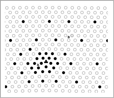
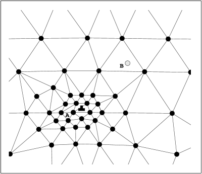
(a)                                                               (b)

Figure 3:

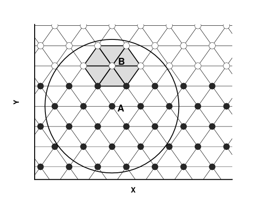
Figure 4:

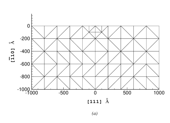
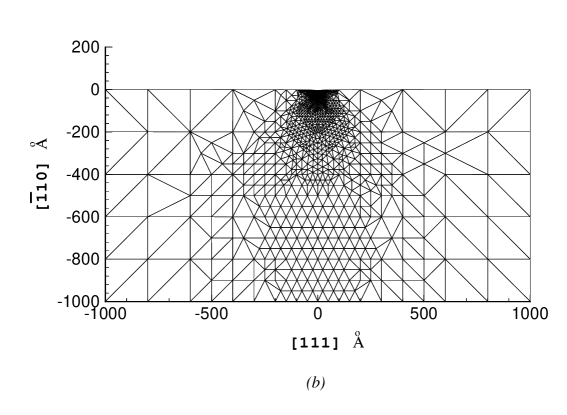
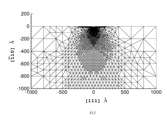
Figure 5:

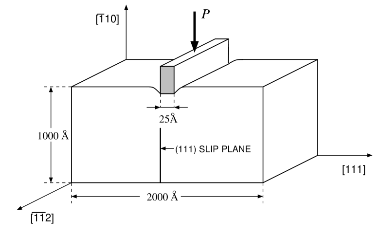
Figure 6:

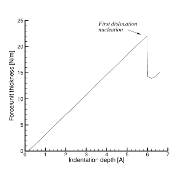
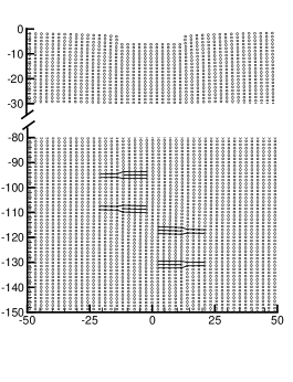
             (a)                                                  (b)

Figure 7:

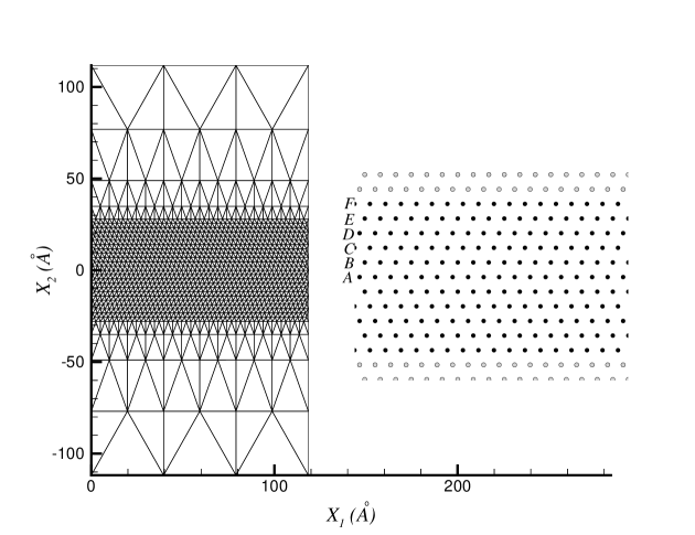
Figure 8:

Figure 9:

(a)                                                                    (b)

Figure 10:

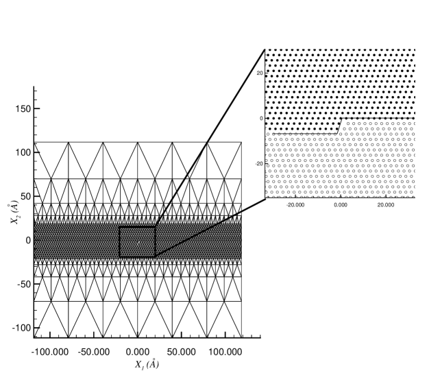
Figure 11:

(a)                                                                                         (b)

Figure 12:

Figure 13:

Figure 14:

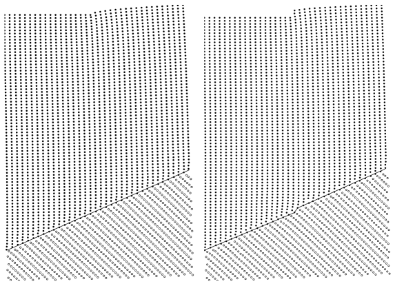
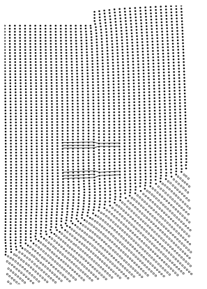
(a)                                         (b)                                         (c)

Figure 15: