Phase-locking in weakly heterogeneous neuronal networks

Abstract

We examine analytically the existence and stability of phase-locked states in a weakly heterogeneous neuronal network. We consider a model of $N$ neurons with all-to-all synaptic coupling where the heterogeneity is in the firing frequency or intrinsic drive of the neurons. We consider both inhibitory and excitatory coupling. We derive the conditions under which stable phase-locking is possible. In homogeneous networks, many different periodic phase-locked states are possible. Their stability depends on the dynamics of the neuron and the coupling. For weak heterogeneity, the phase-locked states are perturbed from the homogeneous states and can remain stable if their homogeneous conterparts are stable. For enough heterogeneity, phase-locked solutions either lose stability or are destroyed completely. We analyze the possible states the network can take when phase-locking is broken.

I Introduction

Phase-locked and synchronized neuronal firing is found throughout the brain and this coherent activity may play an important role in behavior and cognition [1, 2, 3, 4, 5]. Given their importance, it is of interest to understand the mechanisms responsible for their generation. Here, we consider a network of heterogeneous neurons that are coupled synaptically and determine analytically the conditions under which their firing patterns will be phase-locked. Our results could have implications for synchronous phenomena in other areas of biology and physics that are based on pulse-coupled oscillators [6, 7, 8].

Much of the previous analytical work on phase-locking and synchronization in pulse-coupled neuronal oscillators have focused on homogeneous networks [9, 10, 11, 12, 13, 14, 15]. However, any biophysically relevant neuronal network will likely include heterogeneous effects. It is known that heterogeneity can greatly reduce synchrony in networks of phase-coupled oscillators [6, 16, 17]. Coexistence of synchronous and asynchronous states have been shown to exist in large networks of heterogeneous pulse-coupled oscillators [18, 19]. Recently it has been shown numerically that heterogeneous assemblies of neurons can fire coherently. However, the coherent activity can be greatly reduced even when the heterogeneity is very small [20, 21]. Here, we examine analytically the existence and stability of phase-locked solutions of weakly heterogeneous neuronal networks. We consider an all-to-all coupled network of size $N$ where the heterogeneity is in the intrinsic firing frequency of the component neurons. We examine both inhibitory and excitatory connections.

Phase-locking in homogeneous synaptically coupled neuronal networks has been studied analytically with different formalisms [10, 11, 12, 22]. Here, we generalize the formalism developed by Gerstner et al. [12] to examine the existence and stability of phase-locked solutions. We find the conditions for stability of homogeneous phase-locked solutions and examine what happens as we allow the heterogeneity to increase. Our formalism can analyze all periodic phase-locked states but we mainly focus on the synchronized or in-phase state, the anti-synchronized state, and the splay-phase or anti-phase state. We find that stable phase-locking depends crucially on the time course of the synaptic coupling and on the response properties of the neuron to synaptic inputs.

Neurons have recently been classified in accordance with their phase response properties [11]. Type I neurons have the property that their phase response curves are always positive, i.e. the next firing time of the neuron is always advanced in response to a positive (depolarizing) input. In contrast, for Type II neurons the next firing time is either delayed or advanced depending on when the input is received. It has also been shown that Type I neurons admit arbitrarily low frequencies while Type II neurons do not [23]. Our results confirm previous observations that for Type I neurons, excitatory coupling is generally desynchronizing while inhibitory coupling is synchronizing [10, 11, 12]. For Type II neurons, the opposite can be true although not necessarily. In previous work, the requirements on the rise and decay time of the synaptic coupling for stable phase-locking have been separately emphasized [10, 12, 22]. We find that depending on the nature of the synaptic coupling conditions on both are required. A new result for homogeneous neurons is that the splay-phase or anti-phase state can be stable for inhibitory coupling for any finite sized network. For infinite $N$, the splay-phase state is known to be unstable [26, 29].

With weak heterogeneity, phase-locked solutions can exist but with small phase dispersion around their homogeneous counterparts. Stability is possible if the original homogeneous solutions are stable. The addition of heterogeneity cannot stabilize an unstable homogeneous phase-locked state. As the heterogeneity is increased, phase-locked states can either lose stability or cease to exist. Heterogeneity can also foster clustering. When stable phase-locking is lost, the network can enter asynchronous, harmonically locked or suppressed states. Fig. 1 shows examples of various states for two coupled inhibitory neurons obtained from numerical simulations of a biophysically based neuron model given in Appendix A.

In Sec. II we introduce the model and formalism we use for our analysis. In Sec. III we give the conditions which must be satisfied for a periodic phase-locked solution. In Sec. IV we give general conditions for stability of locked solutions. In Sec. V we apply our conditions for the existence and stability of phase-locked states to two coupled homogeneous and heterogeneous neurons. We also examine suppression and harmonic locking. In Sec. VI we examine phase-locking and other dynamics in a network of N neurons. We discuss our results and conclude in Sec. VII.

II Model

Our network consists of $N$ all-to-all coupled neurons. Each time a given neuron fires, a synaptic pulse is transmitted to all the other neurons. The effect of the synapse remains over a finite amount of time. The dynamics of neurons are generally described by biophysically based (Hodgkin-Huxley type) equations which are a set of differential equations for the current balance of the membrane potential and for the dynamics of the component ion channels [24]. In Appendix A, we give a set of biophysically based equations [21]. We use these equations in numerical simulations to confirm our analytical results. These neurons are Type I in contrast to classic Hodgkin-Huxley equations which are Type II [11, 23].

Generally, the differential equations for neuron models are complicated and cumbersome for theoretical analysis. Instead, we use the spike response method for our neuronal dynamics [12, 25, 26]. This formalism is fairly general and can be applied to biophysical neuron models. In this method, the neuron is considered to be a device which fires when a single scalar variable (membrane potential) crosses a threshold from below. The dynamics of the membrane potential consists of a sum of two sets of kernels akin to an integral expansion:

$$v_{i}(t)=\sum_{l}\eta_{i}(t-t_{l}^{i})+\sum_{j,l^{\prime}}\epsilon_{ij}(t-t_{l^{\prime}}^{j}),$$ (1)

where $t^{i}_{l}$ marks the firing times of neuron $i$ (i.e. the $l$th time neuron $i$ reaches the threshold $\theta_{i}$) and $j$ is summed from 1 to $N$ excluding $i$. The kernels are nonzero only for $t-t_{l}^{k}>0$. The kernel $\eta_{i}(t)$ describes the intrinsic dynamics of the neuron after it has been triggered to fire. It represents the ensuing spike (action potential) and recovery behavior. The kernel $\epsilon_{ij}(t)$ represents the response due to synaptic inputs. We do not include the effects of self-coupling in (1) but can do so by modifying $\eta_{i}(t)$. Figure 2 gives examples of kernels.

To linear order we can write $\epsilon_{ij}(t)$ in the form

$$\epsilon_{ij}(t)=\int_{0}^{t}G(s)I_{ij}(t-s)ds,$$ (2)

where $I_{ij}(t)$ is the synaptic input to neuron $i$ from neuron $j$, and $G(t)$ is the linear response function. It has been shown that the linear response is often an adequate approximation for the full nonlinear response [12, 26, 27]. In biophysically based neurons, the synaptic input current is usually given by $I_{ij}(t)=g_{s}S_{ij}(t)(v_{i}-v_{s})$ where $v_{s}$ is a constant reversal potential, $g_{s}$ is the maximal synaptic conductance, and $S_{ij}(t)$ is the synaptic gating variable obtained from a differential equation (see Eq. (A4) in Appendix A). Models often use the simplification $I_{ij}(t)\simeq gS_{ij}(t)$ since $(v_{i}-v_{s})$ is approximately constant away from a spike [11]. The dynamics of the synaptic gating variable has previously been approximated by a recursive scheme where $S_{ij}(t)$ is updated each time the neuron receives an input with $S_{ij}(t)\rightarrow S_{ij}(t)+S_{f}(t-t^{j})$, where $t^{j}$ is the time of the pre-synaptic spike, and $S_{f}(t)$ is a stereotypical synaptic response [10, 11, 29]. We call this type of synaptic model nonsaturating since $S_{ij}(t)$ increases without bound as the firing rate increases. On the other hand the synaptic model given by (A4) is saturating. Here $S_{ij}(t)$ saturates to a finite value as the firing rate of the pre-synaptic neuron increases. In the limit of very fast synaptic rise times we can use the approximation $S(t)\rightarrow S_{f}(t-t^{j})$ to model the dynamics of (A4) [28]. In this case the synapse has no memory of previous activity.

In our network, we allow for heterogeneity in the thresholds of the neurons which implies heterogeneity in the intrinsic firing frequencies. We maintain homogeneity in the time courses of the kernels. We can make the threshold heterogeneity explicit with the transformation $v_{i}\rightarrow v_{i}-I_{i}$ and $\theta_{i}\rightarrow\theta-I_{i}$, where $I_{i}$ can be thought of as a normalized applied driving current, and $\theta$ is a constant threshold. We make the synaptic strengths of the neurons explicit by setting $\epsilon_{ij}(t)=J\epsilon(t)$, where $J$ represents the coupling strength. Heterogeneous coupling could be accounted for by setting $J=J_{ij}$. When $J>0$ we call this excitatory coupling and for $J<0$ we call this inhibitory coupling. Putting this in Eq. (1) yields

$$v_{i}(t)=I_{i}+\sum_{l}\eta(t-t_{l}^{i})+\sum_{j,l^{\prime}}J\epsilon(t-t_{l^{\prime}}^{j}),$$ (3)

In this form, the network heterogeneity is explicitly expressed in the applied current $I_{i}$. We can set the threshold for all the oscillators to 1 by a simple rescaling without any loss of generality. In this formulation, $I_{ij}(t)$ in Eq. (2) can be thought of as the post-synaptic current while $\epsilon_{ij}(t)$ can be thought of as the post-synaptic potential. Often we will refer to the rise time of the synaptic current which will mean the rise time of $I_{ij}(t)$. We note that the synaptic kernel $\epsilon_{ij}(t)$ will itself have a rise time which can depend on both the rise and decay time of the synaptic current.

Remark 1

We have assumed that the synaptic kernel does not depend on the time of arrival or phase of the synaptic input. For the integrate-and-fire model, as will be shown below, this is true. However, in general, there will be a dependence which we can express as $\epsilon_{ij}=\epsilon(t-t^{i}_{l},t-t^{j}_{m})$. For the ensuing analysis, we examine phase-locked solutions where the time since the last spike is fixed. Our assumption is then valid if $|\partial_{u}\epsilon(u,v)|<<|\partial_{v}\epsilon(u,v)|$. For neurons where the response changes drastically with phase, our analysis will need to be modified.

1 Integrate-and-fire Model

To compare to previous analytical results and to provide a simple concrete example we consider a leaky integrate-and-fire model [10, 11, 12, 30] with dynamics given by

$$\frac{dv_{i}}{dt}=I_{i}-v_{i}-\sum_{l}\delta(t-t^{i}_{l})+\sum_{j,l^{\prime}}JS_{f}(t-t^{j}_{l^{\prime}}),$$ (4)

where the firing times $t^{i}_{l}$ indicate when $v_{i}$ reaches the threshold value which we have set arbitrarily to 1. Each time the potential reaches threshold a delta function pulse is subtracted to reset the potential. As an example for a saturating synaptic current, consider a double exponential function

$$S_{f}(t)=\left\{\begin{array}[]{ll}\exp(-\beta t)-\exp(-\alpha t),&0<t<t_{f},\\ 0,&t_{f}<t,\end{array}\right.$$ (5)

where $\alpha>\beta$ and $t_{f}$ is the time elapsed to the next synaptic input. For nonsaturating synapses, we can set $t_{f}=\infty$ [10, 11].

Equation (4) can be integrated directly [12, 26] to obtain the kernels :

$$\eta(t)=-\exp(-t),\quad t>0,$$ (6)

$$\epsilon(t)=\left\{\begin{array}[]{ll}\frac{1}{1-\beta}[\exp(-\beta t)-\exp(-t)]-\frac{1}{1-\alpha}[\exp(-\alpha t)-\exp(-t)],&0<t<t_{f},\\ \left(\frac{1}{1-\beta}\left[\exp(-\beta t_{f})-\exp(-t_{f})\right]-\frac{1}{1-\alpha}\left[\exp(-\alpha t_{f})-\exp(-t_{f})\right]\right)\exp(-(t-t_{f})),&t_{f}<t.\end{array}\right.$$ (7)

We show examples of the kernels in Fig. 2. Note that for $\alpha>\beta$, $\epsilon(t)>0$ so that the time of the next firing is always advanced in response to a positive synaptic input and thus the integrate-and-fire model can be classified as Type I.

III Existence of Phase-locked Solutions

We first examine the existence of periodic phase-locked solutions. We derive a condition which all periodic phase-locked solutions must satisfy. Our condition generalizes that of Gerstner et al. [12] to include heterogeneity in the applied current and locking at arbitrary phases. Van Vreeswijk et al. [10] derived a locking condition for the specific case of two homogeneous integrate-and-fire neurons locked at arbitrary phases.

Our strategy is to assume that there is a periodic phase-locked solution and then check for self-consistency, i.e. the membrane potential must be 1 (the threshold value) at the time of the next firing. Consider each neuron labeled by $i$ to be firing periodically in the past at $t_{l}^{i}=(\phi_{i}-l)T$, where $l=1,2,\ldots$, and $0\leq\phi_{i}<1$ is a phase shift. Inserting these firing times into Eq. (3) gives

$$v_{i}(t)=I_{i}+\sum_{l\geq 1}\eta(t-(\phi_{i}-l)T)+\sum_{j\neq i,l^{\prime}\geq 0}J\epsilon(t-(\phi_{j}-l)T),\quad t\leq\phi_{i}T$$ (8)

This assumes that each neuron will fire once within a period. We will discuss the situation where this does not occur later.

Neuron $i$ will fire next at $t=\phi_{i}T$. Inserting this into Eq. (8) and imposing self-consistency yields

$$v_{i}(\phi_{i}T)=1=I_{i}+\sum_{l\geq 1}\eta(lT)+\sum_{j\neq i,l^{\prime}\geq 0}J\epsilon(l^{\prime}T+(\phi_{i}-\phi_{j})T)$$ (9)

Note that for $(\phi_{i}-\phi_{j})<0$, the first term of the $\epsilon$ kernel sum will be equivalently zero by definition of the kernels. The interpretation is that within the given period ($l^{\prime}=0$), neuron $j$ spikes after neuron $i$ and the synaptic effect does not appear until the next period, $l^{\prime}=1$. If Eq. (9) is satisfied then a phase-locked solution exists. The solution will be specified by the set of phases ${\phi_{i}}$ and the period $T$. We note that the phase locking condition given by Eq. (9) consists of $N$ equations for $N$ phases and the period. However, the system is translationally invariant in time so one of the phases can be arbitrarily fixed. This then leaves us with a well defined system of $N$ equations and $N$ unknowns ($N-1$ phases and the period $T$).

For a homogeneous system, the equations are symmetric with respect to the neuron index, implying a large number of possible solutions for the phases. The most notable solutions are the in-phase [6, 9, 10, 11, 12, 16] or synchronized state where all the phases are the same and the splay-phase state [31, 32, 33, 34] where the phases are spaced evenly apart over one period. There are also clustered solutions where equal numbers of neurons will fire at evenly spaced phases. An example is the anti-synchronous [10, 35, 36, 37, 38, 39] state where half the oscillators fire a half a period apart. The inclusion of heterogeneity breaks the permutation symmetry. However, for small enough heterogeneity, near synchronous, anti-synchronous and splay-phase solutions that are perturbed from their homogeneous counterparts can exist.

A Phase-locked solutions for two neurons

As a specific example, we consider the existence of periodic phase-locked solutions for the case of two coupled neurons. We consider neurons with heterogeneous applied current $I_{1}\geq I_{2}$ and homogeneous coupling. We suppose the neurons have fired at times $t_{l}^{i}=(\phi_{i}-l)T$, where $l=1,2,3,\ldots$, $i=1,2$. We choose the origin of time so that $\phi_{2}\geq\phi_{1}$, i.e. neuron 2 always fires after (or with) neuron 1.

Applying condition (9) for $N=2$ yields

$$v_{1}(\phi_{1}T) = 1=I_{1}+\sum_{l\geq 1}[\eta(lT)+J\epsilon(lT-\phi T)],$$ (10)

$$v_{2}(\phi_{2}T) = 1=I_{2}+\sum_{l\geq 1}\eta(lT)+\sum_{l\geq 0}J\epsilon(lT+\phi T)],,$$ (11)

where $\phi=\phi_{2}-\phi_{1}\geq 0$ and we have taken into account that neuron 2 fires after neuron 1. We must solve Eqs. (10) and (11) for the phase $\phi$ and period $T$.

A relation for the phase can be derived by subtracting Eq. (11) from (10) to give

$$0=I_{1}-I_{2}-G(\phi)$$ (12)

where

$$G(\phi)=J\sum_{l\geq 1}[\epsilon(lT-T+\phi T)-\epsilon(lT-\phi T)].$$ (13)

For homogeneous neurons, ($I_{1}=I_{2}$), condition (12) for the phase is equivalent to that derived by Van Vreeswijk et al. [10]. For $\epsilon(0)=0$ (which is generally true), we find that $G(0)=G(0.5)=G(1)=0$. In addition, $G(\phi)$ is symmetric around $G(0.5)$. This implies that for homogeneous neurons $\phi=0$ and $\phi=0.5$ are phase-locked solutions which we refer to as the synchronized and anti-synchronized solutions respectively. If additional phase-locked solutions exist they must always appear symmetrically in pairs on either side of $\phi=0.5$. From Eq. (12), it is apparent that neurons with heterogeneous $I_{i}$ cannot lock in a purely synchronous or anti-synchronous state. However, if the heterogeneity is not too large, there can still be phase-locked solutions near to synchrony and near to anti-synchrony. For heterogeneous neurons it is also possible that phase-locked solutions do not exist at all. As a specific example, consider the integrate-and-fire model. Using $\epsilon(t)$ without saturation from (7) in condition (13), we find

$$G(\phi)=\frac{J}{1-\alpha}\left[\frac{e^{\alpha\phi T-\alpha T}-e^{-\alpha\phi T}}{1-e^{-\alpha T}}-\frac{e^{\phi T-T}-e^{-\phi T}}{1-e^{-T}}\right]-\frac{J}{1-\beta}\left[\frac{e^{\beta\phi T-\beta T}-e^{-\beta\phi T}}{1-e^{-\beta T}}-\frac{e^{\phi T-T}-e^{-\phi T}}{1-e^{-T}}\right]$$ (14)

Figure 3 shows some examples of $G(\phi)$ for various, $T$, $\alpha$ and $\beta$.

To specify the period we add Eq. (11) to (10) and divide by 2 to obtain

$$1=\bar{I}+\sum_{l\geq 1}\{\eta(lT)+\frac{J}{2}[\epsilon(lT-\phi T)+\epsilon(lT-T+\phi T)]\},$$ (15)

where $\bar{I}=(I_{1}+I_{2})/2$. Using Eq. (15) and assuming the rise time of the synaptic current is very short compared to the decay time ($\alpha>>\beta$), we find that the period for the synchronized state ($\phi=0$) for the integrate-and-fire model with saturating synapses satisfies [28]

$$1=\bar{I}(1-e^{-T})+\frac{J(e^{-\beta T}-e^{-T})}{(1-\beta)}.$$ (16)

The period for nonsaturating synapses is given by Eq. (16) with an extra factor of $(1-e^{-\beta T})$ in the denominator of the second term. The period does not change much for near synchrony where the phase is near zero. It has been found that (16) can be used to estimate the period of a synchronized inhibitory network of biophysically based Type I neuron models [28].

IV Stability of phase-locking

We examine the local stability of phase-locked solutions for a network of $N$ all-to-all coupled neurons. Our formalism generalizes that of Ref. [12] to include heterogeneity in the applied current $I_{i}$ and for locking at arbitrary phases $\phi_{i}$. In this strategy, perturbations around the firing times of the phase-locked solutions are checked for growth or decay. Based on the perturbation dynamics we obtain sufficient conditions for stability.

For neuron $i$ we consider firing in the past at times

$$t_{l}^{i}=(\phi_{i}-l)T+\delta_{i}(n-l),\quad l=1,2,3,\ldots,$$ (17)

where $\delta_{i}(n-l)$ is a small perturbation around each firing time and $n$ is the index for the current perturbation. We want to examine whether $\delta_{i}(n)$ grows or decays as $n\rightarrow\infty$. We will show that $\delta_{i}(n)$ depends on the perturbations of all of the previous firing times of all of the neurons in the network. To derive a mapping for $\delta_{i}(n)$, we insert the perturbed firing times (17) into Eq. (3) to obtain

$$v_{i}(t)=I_{i}+\sum_{l\geq 1}\eta(t-(\phi_{i}-l)T-\delta_{i}(n-l))+\sum_{j\neq i,l^{\prime}\geq 0}J\epsilon(t-(\phi_{j}-l^{\prime})T-\delta_{j}(n-l^{\prime})).$$ (18)

The neuron will next fire at $t=\phi_{i}T+\delta_{i}(n)$. Hence we can set $v_{i}(\phi_{i}T+\delta_{i}(n))=1$, which implies after linearizing in $\delta_{i}(n)$ that

$$v_{i}(\phi_{i}T)\simeq 1-\dot{v}_{i}(\phi_{i}T)\delta_{i}(n),$$ (19)

where the dot denotes the first derivative with respect to time. We now set $t=\phi_{i}T$ in Eq. (18). Using Eq. (19) and linearizing in $\delta_{k}(l)$ we obtain

$$1-\dot{v}_{i}(\phi_{i}T)\delta_{i}(n)=I_{i}+\sum_{l\geq 1}[\eta(lT)-\dot{\eta}(lT)\delta_{i}(n-l)]$$ (21)

$$\mbox{}+\sum_{j\neq i,l^{\prime}\geq 0}J[\epsilon(l^{\prime}T+(\phi_{i}-\phi_{j})T)-\dot{\epsilon}(l^{\prime}T+(\phi_{i}-\phi_{j})T)\delta_{j}(n-l^{\prime})].$$

For an unperturbed spiking history Eq. (9) holds. This allows us to simplify Eq. (21). Solving for $\delta_{i}(n)$ yields

$$\delta_{i}(n)=\frac{1}{\dot{v}_{i}(\phi_{i}T)}\left[\sum_{l\geq 1}\dot{\eta}(lT)\delta_{i}(n-l)+\sum_{j\neq i,l^{\prime}\geq 0}J\dot{\epsilon}(l^{\prime}T+(\phi_{i}-\phi_{j})T)\delta_{j}(n-l^{\prime})\right],$$ (22)

where

$$\dot{v}_{i}(\phi_{i}T)=\sum_{l\geq 1}\dot{\eta}(lT)+\sum_{j\neq i,l^{\prime}\geq 0}J\dot{\epsilon}(l^{\prime}T+(\phi_{i}-\phi_{j})T),$$ (23)

Stability is determined from Eqs. (22) and (23). It is not immediately transparent since a given perturbation of a neuron depends on all previous perturbations including those within the same cycle (i.e have the same index $n$). However, by turning the dynamics into a first return map we can obtain a sufficient condition for stability which we state in the following theorem.

Theorem 1

If the series (22) can be truncated then a sufficient condition for stability of a phase-locked state is that all of the coefficients of the series in (22) are positive.

Proof: We first make $\delta_{i}(n)$ depend only on previous firings by substituting for $\delta_{j}(n)$ recursively on the right-hand side of the mapping (22) whenever $\phi_{i}>\phi_{j}$. This substitution can be done systematically if we index the neurons so that they are ordered by phase with $\phi_{1}<\phi_{2}<\cdots<\phi_{N}$, i.e. neuron 1 fires first, neuron 2 second, and so forth. With this phase ordering the mapping for $\delta_{1}(n)$ is given by Eq. (22) with $i=1$ and $l^{\prime}\geq 1$. Since neuron 1 fires first it only depends on the previous firings of the other neurons. To obtain the mapping for $\delta_{2}(n)$ we must substitute for $\delta_{1}(n)$ on the right hand side of mapping (22) with $i=2$. We continue this recursive substitution scheme for all $N$ neurons where for $i=k$ we must substitute for $\delta_{j}(n)$ on the right hand side of Eq. (22) for $j<k$. We write the resulting mapping as

$$\delta_{i}(n)=\sum_{j=1}^{N}\sum_{l=1}^{\infty}M_{ij}(l)\delta_{j}(n-l),$$ (24)

where $M_{ij}(l)$ is obtained from applying the prescription described above and the sum over $j$ now includes $i$. The elements of $M_{ij}$ are composed of products and sums of the coefficients in the series (22). Thus, if the coefficients are positive then the elements of $M_{ij}$ are positive. Proposition 1 then directly follows from the following lemma. $\Box$

Lemma 1

If the series (22) can be truncated then a sufficient condition for stability is given by $M_{ij}(l)>0$.

Proof: By assumption the kernels $\eta(t)$ and $\epsilon(t)$ vanish sufficiently quickly so that we can truncate the series in Eq. (22). This allows us to truncate the inner sum in Eq. (24) at some $l=l_{M}$. We can then express the mapping (24) in terms of a first return mapping by embedding in a higher dimension with

$$\vec{\delta}(n)={\mathcal{M}}\cdot\vec{\delta}(n-1)$$ (25)

where in block form,

$$\vec{\delta}(n)=\left(\begin{array}[]{c}{\mathbf{\delta}}(n)\\ {\mathbf{\delta}}(n-1)\\ {\mathbf{\delta}}(n-2)\\ \vdots\\ {\mathbf{\delta}}(n-l_{M}+1)\end{array}\right),\qquad{\mathcal{M}}=\left(\begin{array}[]{ccccc}{\bf M}(1)&{\bf M}(2)&\cdots&{\bf M}(l_{M}-1)&{\bf M}(l_{M})\\ {\bf I}&0&\cdots&0&0\\ 0&{\bf I}&\cdots&0&0\\ \vdots&\vdots&&\vdots&\vdots\\ 0&0&\cdots&{\bf I}&0\end{array}\right),$$ (26)

${\bf I}$ denotes the $N\times N$ identity matrix, ${\bf\delta}(k)$ is the column vector of length $N$ with elements $\delta_{i}(k)$ and ${\bf M}(l)$ is the $N\times N$ matrix with elements $M_{ij}(l)$ from Eq. (24).

The dynamics of the perturbations are determined by repeated matrix multiplications of ${\mathcal{M}}$. The phase-locked solution is stable if all of the eigenvalues of ${\mathcal{M}}$ have absolute value less than unity. For simple enough systems we can calculate the eigenvalues explicitly (see Appendix B). This is usually not the case so we need to determine bounds on the modulus of the maximum eigenvalue $\rho({\mathcal{M}})$ (spectral radius). The spectral radius is less than or equal to any given matrix norm [40]. In particular $\rho({\mathcal{M}})\leq\|{\mathcal{M}}\|_{\infty}=\max\sum_{j}|{\mathcal{M}}_{ij}|$. From Eqs. (22), (23) and (24) we find that the rows of $\sum_{l}{\bf M}(l)$ sum to unity, which implies that all of the rows ${\mathcal{M}}$ also sum to unity. Thus we immediately find that 1 is an eigenvalue with eigenvector $\vec{\delta}=(1,1,1,\ldots,1)$. This corresponds to a global uniform shift in time and is due to the time translational invariance of the dynamics. It can be disregarded for stability considerations [12]. If the elements of ${\mathcal{M}}$ are non-negative then $\rho({\mathcal{M}})=\|{\mathcal{M}}\|_{\infty}=1$. The spectral radius is the unique maximum modulus eigenvalue if ${\mathcal{M}}$ is a primitive matrix which is satisfied if ${\mathcal{M}}^{m}>0$ for some $m$ [40]. By inspection of ${\mathcal{M}}$ from (26), we see that ${\mathcal{M}}^{m}>0$ if $M_{ij}(l)>0$ proving Lemma 1. $\Box$

It is important to note that $M_{ij}(l)>0$ is not a necessary condition for stability. We make this explicit in the following corollary.

Corollary 1

Stability is possible even if $M_{ij}$ has negative elements.

Proof: If ${\mathcal{M}}$ is primitive we know that one eigenvalue is always 1, it is nondegenerate and all the other eigenvalues are within the unit disc. Stability is lost if an interior eigenvalue crosses the unit boundary, which can occur if we allow some of the elements of $M_{ij}$ to become negative. Because the eigenvalues are continuous functions of the elements, we can make some of the elements negative and still keep the eigenvalues within the unit disc by the intermediate value theorem. $\Box$

Remark 2

Our perturbation scheme generalizes that of Gerstner et al. [12] who arrived at the stability equation (25) for the purely synchronized solution (all phases equal). They considered dynamics where $\dot{\epsilon}(0)=0$ so only previous perturbations affect the current one. For a homogeneous network, they proved the necessary and sufficient condition for stability is $J\sum_{l}\dot{\epsilon}(lT)>0$. In our case with heterogeneity, pure synchrony is not possible. We are thus forced to consider locking at arbitrary phases and use the recursive substitution scheme above to calculate the mapping for the perturbations.

A Stability for two coupled neurons

As an example we apply the formalism for $N=2$. Equation (22) is

$$\delta_{1}(n) = \frac{1}{\dot{v}_{1}}\sum_{l\geq 1}[\dot{\eta}(lT)\delta_{1}(n-l)+J\dot{\epsilon}(lT-\phi T)\delta_{2}(n-l)],$$ (27)

$$\delta_{2}(n) = \frac{1}{\dot{v}_{2}}\sum_{l\geq 1}\dot{\eta}(lT)\delta_{2}(n-l)+\frac{J}{\dot{v}_{2}}\sum_{l^{\prime}\geq 0}\dot{\epsilon}(l^{\prime}T+\phi T)\delta_{1}(n-l^{\prime}),$$ (28)

where $\phi=\phi_{2}-\phi_{1}$. Since neuron 2 fires after neuron 1, we substitute $\delta_{1}(n)$ from Eq. (27) into Eq. (28) to yield

$$\delta_{2}(n)=\sum_{l\geq 1}\left\{\left[\frac{\dot{\eta}(lT)}{\dot{v}_{2}}+\frac{J^{2}\dot{\epsilon}(\phi T)\dot{\epsilon}(lT-\phi T)}{\dot{v}_{1}\dot{v}_{2}}\right]\right.\delta_{2}(n-l)$$ (30)

$$\mbox{}+\left.\left[\frac{J\dot{\epsilon}(lT+\phi T)}{\dot{v}_{2}}+\frac{J\dot{\epsilon}(\phi T)\dot{\eta}(lT)}{\dot{v}_{1}\dot{v}_{2}}\right]\delta_{1}(n-l)\right\}.$$

Combining (27) with (30) we obtain

$${\bf M}(l)=\left(\begin{array}[]{cc}\frac{\dot{\eta}(lT)}{\dot{v}_{1}}&\frac{J\dot{\epsilon}(lT-\phi T)}{\dot{v}_{1}}\\ \frac{J\dot{\epsilon}(lT+\phi T)}{\dot{v}_{2}}+\frac{J\dot{\epsilon}(\phi T)\dot{\eta}(lT)}{\dot{v}_{1}\dot{v}_{2}}&\frac{\dot{\eta}(lT)}{\dot{v}_{2}}+\frac{J^{2}\dot{\epsilon}(\phi T)\dot{\epsilon}(lT-\phi T)}{\dot{v}_{1}\dot{v}_{2}}\end{array}\right)$$ (31)

which is to be used in Eqs. (25) and (26). The sufficient condition for stability of a phase-locked solution is given by Lemma 1 which we denote by ${\bf M}(l)>0$.

For the case of two neurons we can also obtain the necessary condition for stability by examining whether or not one neuron can remain locked to the other one independently of whether they are firing periodically. This type of stability was considered by van Vreeswijk et al. [10]. We derive their condition using the spike response formalism which we state in the following theorem.

Theorem 2

A necessary condition for stability of a periodic phase-locked solution for two neurons is $G^{\prime}(\phi)>0$, where $G(\phi)$ is given by Eq. (13) and prime denotes the first derivative with respect to $\phi$.

Proof: Suppose that neuron $1$ fires at times $t^{1}_{l}=t_{1-l}$ and neuron $2$ fires at times $t^{2}_{l}=t_{1-l}+\theta+\delta(n-l)$, where $l\geq 0$. We consider the situation where neuron $2$ has fired after neuron $1$. Neuron $1$ will satisfy the condition $v_{1}(t_{1})=1$ while neuron $2$ satisfies the condition $v_{2}(t_{1}+\theta+\delta(n))=1$, from which we derive the linearization $v_{2}(t_{1}+\theta)=1-\dot{v}_{2}(t_{1}+\theta)\delta(n)$. Inserting this into Eq. (3) and linearizing in $\delta(n-l)$ yields

$$1 = I_{1}+\sum_{l\geq 1}[\eta(t_{1}-t_{1-l})+J\epsilon(t_{1}-t_{1-l}-\theta)-J\dot{\epsilon}(t_{1}-t_{1-l}-\theta)\delta(n-l)],$$ (32)

$$1-\dot{v}_{2}(t_{1}+\theta)\delta(n) = I_{2}+\sum_{l\geq 1}[\eta(t_{1}-t_{1-l})-\dot{\eta}(t_{1}-t_{1-l})\delta(n-l)+J\epsilon(t_{1}-t_{2-l}+\theta)].$$ (33)

Subtracting Eq. (33) from Eq. (32) and canceling terms, we obtain the condition for synchrony:

$$I_{1}-I_{2}=J\sum_{l\geq 1}[\epsilon(t_{1}-t_{2-l}+\theta)-\epsilon(t_{1}-t_{1-l}-\theta)],$$ (34)

and the perturbation mapping:

$$\delta(n)=\frac{1}{\dot{v}_{2}(t_{1}+\theta)}\sum_{l\geq 1}[\dot{\eta}(t_{1}-t_{1-l})-J\dot{\epsilon}(t_{1}-t_{1-l}-\theta)]\delta(n-l),$$ (35)

where

$$\dot{v}_{2}(t_{1}+\theta)=\sum_{l\geq 1}[\dot{\eta}(t_{1}-t_{1-l})+J\dot{\epsilon}(t_{1}-t_{2-l}+\theta)].$$ (36)

Eq. (35) can be rewritten as

$$\delta(n)=\sum_{l\geq 1}M(l)\delta(n-l),$$ (37)

where

$$M(l)=\frac{1}{\dot{v}_{2}}[\dot{\eta}(t_{1}-t_{1-l})-J\dot{\epsilon}(t_{1}-t_{1-l}-\theta)].$$ (38)

It will be shown in Lemma 2 that a necessary condition for stability is $\sum M(l)<1$.

Applying this condition leads to

$$\frac{\sum_{l\geq 1}\dot{\eta}(t_{1}-t_{1-l})-J\dot{\epsilon}(t_{1}-t_{1-l}-\theta)}{\sum_{l\geq 1}\dot{\eta}(t_{1}-t_{1-l})+J\dot{\epsilon}(t_{1}-t_{2-l}+\theta)}<1,$$ (39)

which implies

$$J\sum_{l\geq 1}[\dot{\epsilon}(t_{1}-t_{1-l}-\theta)+\dot{\epsilon}(t_{1}-t_{2-l}+\theta)]>0,$$ (40)

For periodic firing we can set $t_{l}=(1-l)T$ and $\theta=\phi T$ in (40) which is equivalent to $G^{\prime}(\phi)/T>0$ which leads to $G^{\prime}(\phi)>0$ as stated in Theorem 2. $\Box$

Lemma 2

For perturbed dynamics of the form

$$\delta(n)=\sum_{l=1}^{l_{M}}M(l)\delta(n-l),$$ (41)

a necessary condition for stability is that $\sum M(l)\leq 1$. If $M(l)>0$, for all $l$, then the condition is sufficient as well.

Proof: The dynamics can be expressed in matrix notation as in Eq. (25) where ${\bf M}(l)$ is replaced by the scalar $M(l)$ and the identity matrices are replaced by 1. The corresponding matrix ${\mathcal{M}}$ is a companion matrix and the characteristic polynomial is given by [12, 40]

$$1=\sum_{l=1}^{l_{M}}M(l)\lambda^{-l}.$$ (42)

Let $f(\lambda)=\sum_{l}M(l)\lambda^{-l}$, so that eigenvalues of ${\mathcal{M}}$ satisfy $f(\lambda)=1$. Suppose $\sum_{l}M(l)>1$. Then $f(\lambda)>1$. However, $f(\lambda)\rightarrow 0$ as $\lambda\rightarrow\infty$. Thus since $f$ is a polynomial and hence continuous, $f(\lambda)=1$ at some $\lambda>1$, or in other words one eigenvalue will be greater than 1. Thus $\sum_{l}M(l)\leq 1$ is necessary for all eigenvalues to be less than 1 and hence for stability. If $M(l)>0$, then $\sum_{l}M(l)<1$ is necessary and sufficient for stability since $f(\lambda)<1$, for all $\lambda\geq 1$. Thus there are no eigenvalues greater than or equal to 1. $\Box$

Remark 3

The condition $G^{\prime}(\phi)>0$ is not a sufficient condition for periodic phase-locking. However, if the dynamics are constrained so that $M(l)$ as given in Eq. (38) is positive for all $l$, then $\sum_{l\geq 1}M(l)<1$ is the necessary and sufficient condition for arbitrary phase-locking. However, this constraint does not ensure periodicity. For instance, it may be possible that two neurons could be locked together in a higher order periodic or even an aperiodic orbit.

V Two neuron network

We now apply our formalism to examine the existence and stability of specific phase-locked solutions for two coupled neurons. We will revisit the case of two homogeneous neurons and then consider neurons with heterogeneous applied current but with homogeneous inhibitory and excitatory coupling. In Appendix B we consider a simple example for two neurons where only the kernels from the last firing are kept. We compute the eigenvalues for stability explicitly and compare with our results for the general case.

Applying the stability conditions for phase-locked solutions, we make the following proposition for the stability of two coupled neurons. Although we treat the spiking period $T$ as a parameter in the proposition, it is important to note that it is an emergent time scale that depends on parameters of the network.

Proposition 1

A periodic phase-locked solution for two coupled neurons is stable if in (31) i) $\dot{\eta}(lT)>0$ for $l\geq 1$, ii) $J\dot{\epsilon}(\phi T)\geq 0$ and iii) $J\dot{\epsilon}(lT\pm\phi T)>0$, for all $l\geq 1$. These are sufficient but not necessary conditions.

Proposition 1 is established by analyzing the matrix elements of ${\bf M}(l)$ in (31). By assumption $\dot{v}_{1}>0$ and $\dot{v}_{2}>0$. Conditions i), ii) and iii) then imply that ${\bf M}(l)>0$ proving the proposition by Lemma 1. Condition i) is generally true for most neuron models. Condition ii) is strongly dependent on the neuron type. Condition iii) is contingent on the neuron type as well as the neuron parameters, i.e. strength of the applied current, the synaptic strength and the synaptic decay time. Gerstner et al. [12] proved Proposition 1 for the homogeneous synchronous case ($\phi=0$) for N coupled neurons where $N$ is large. We discuss this case in Sec. VI A. Condition iii) corresponds to a special case of their locking theorem. This puts a condition on how slow the onset of the synapse can be. As will be discussed below, condition ii) was implicitly assumed in their theorem. Van Vreeswijk et al. [10] emphasized condition ii) in their criterion for stability.

A Homogeneous Neurons

The existence and stability of phase-locking for two homogeneous neurons has been analyzed in detail by van Vreeswijk et al. [10] and by Hansel et al. [11] for excitatory connections. These analytical results used phase reductions or considered integrate-and-fire dynamics. Our formalism is applicable to a more general class of neuron models. In Sec. V B, we consider heterogeneous neurons. Gerstner et al. [12] considered the stability of the synchronous solution for a large homogeneous network. We will relate the stability conditions of Ref. [12] to those of Ref. [10]. Periodic phase-locked solutions are given by Eqs. (12) and (15) for $I_{1}=I_{2}$. As discussed in Sec. III A, these include the synchronous ($\phi=0$) and anti-synchronous ($\phi=0.5$) solutions as well as a possible third locked solution.

1 Inhibitory Coupling

Here we relate the results and formalism of van Vreeswijk et al. [10] to our formalism. First consider synchronous locking. As mentioned, condition i) in Proposition 1 is satisfied for most neuron models. For Type I models, $\epsilon(t)$ is always positive so condition ii) can only be satisfied if $\dot{\epsilon}(0)=0$. This condition is equivalent to a nonzero rise time of the synaptic current which was emphasized by Van Vreeswijk et al. [10] as the condition required for synchrony with inhibition. In order for synchrony to occur with inhibition, the effect of the first neuron on the second one cannot be felt immediately. They gave an empirical criterion that the synaptic rise time be slower than the width of the spike. For certain Type II models where $\epsilon(t)$ is initially negative and then becomes positive $J\dot{\epsilon}(0)$ could be greater than zero (see Fig. 2). Condition iii) is easily satisfied for Type I neurons (which includes the integrate-and-fire model). Recall that inhibitory coupling is given by $J<0$. Thus, if $\epsilon(t)$ is positive with a maximum at $t=t_{c}$ and is monotone decreasing for $t>t_{c}$ (which applies to Type I neurons) then condition iii) in Proposition 1 is equivalent to $T-\phi T>t_{c}$. The decay rate of $\epsilon(t)$ is controlled to some extent by the decay rate of the synaptic current as well as the intrinsic membrane decay rate (see Eq. (7)). The period on the other hand is an emergent property of the network which depends on the applied current, synaptic strength, and synaptic time scales [28]. For Type I neurons it can be estimated from Eq. (16). For certain Type II neurons it may be possible that condition iii) can never be satisfied so synchronous solutions would not be possible with inhibition.

Proposition 1 gives sufficient conditions for stability. By Corollary 1, synchrony may be possible even if Proposition 1 is violated. To find when locking is not possible we examine the necessary condition given by Theorem 2. From Eq. (13) we note that the necessary condition for stability

$$G^{\prime}(0)\equiv JT\dot{\epsilon}(0)+2JT\sum_{l\geq 1}\dot{\epsilon}(lT)>0.$$ (43)

is satisfied for Proposition 1 as expected. If $\dot{\epsilon}(0)>-2\sum_{l\geq 1}\dot{\epsilon}(lT)$ then synchrony is unstable. Satisfying this condition depends on $\dot{\epsilon}(0)$ which is governed by the rise time of the synaptic current. In order for stability, the neuron must be able to fire without being immediately and strongly inhibited by the synapse. This relates to the van Vreeswijk et al. [10] statement that the rise of the synapse must be slower than the generation of a spike for stability to be possible. For the integrate-and-fire model with nonsaturating synapses, a zero rise time guarantees instability. This can be seen by examining Eq. (14) where it can be shown that $G^{\prime}(0)<0$ if $\alpha\rightarrow\infty$ and $T>0$. This verifies previous results of local instability of the synchronous state for zero rise time with inhibition in the integrate-and-fire model [10, 12].

By Proposition 1, the anti-synchronous solution is stable as long as the synapse is fast enough so that $\dot{\epsilon}(0.5T+lT)<0$, for $l\geq 0$. From (13) we find the necessary condition for stable anti-synchrony is given by

$$G^{\prime}(0.5)\equiv 2JT\sum_{l\geq 1}\dot{\epsilon}(lT-0.5T)>0.$$ (44)

Condition (44) shows that $G^{\prime}(0.5T)$ could be negative if the onset of inhibition is very slow. For the integrate-and-fire model this requires that $\alpha$ and $\beta$ be small enough in Eq. (7) (See Fig. 3). This is in accordance with the results of van Vreeswijk et al. [10].

The synchronized and anti-synchronized solutions can both be stable simultaneously if the rise time is nonzero and $\epsilon(t)$ is monotone decreasing for $t\geq 0.5T$. If this is the case then additional phase-locked solutions must also exist. Since $G(\phi)$ is continuous, if $G^{\prime}(\phi)$ is positive at $0$, $0.5$ and $1$ then it must cross zero at least once between 0 and 0.5 and between 0.5 and 1. If it crosses only once then this solution must be unstable. (See Fig. 3). Since $G(\phi)$ is symmetric about $\phi=0.5$, we can think of these two solutions as one. This third solution was obtained numerically in the integrate-and-fire model with nonsaturating synapses in Refs. [10, 11] where it was found to arise from a pitchfork bifurcation of the anti-synchronous solution. It approaches the synchronous solution as the synapse becomes faster compared to the period ($\alpha$ and $\beta$ get larger). The location of the third solution with respect to the synchronous and anti-synchronous demarcates the basin of attractions for the two stable solutions. All phase-locked solutions can be unstable if the onset of the synapse is so slow that $\epsilon(t)$ is still increasing at $t=T$ because ${\bf M}$ is no longer a positive matrix. For slow enough synapses, the necessary conditions for stability given by (43) and (44) can both be violated.

2 Excitatory Coupling

The case of slow excitatory coupling for two neurons has been analyzed previously by van Vreeswijk et al. [10] and Hansel et al. [11]. They both show that for Type I neurons, synchrony is generally unstable and anti-synchrony is stable for slow synapses. Our analysis agrees with their results. For two neurons, stability is not ensured since $\dot{\epsilon}(lT)<0$, violating Proposition 1. From Eq. (43) we find that the necessary condition for synchrony in Theorem 2 is violated for excitatory coupling unless $\dot{\epsilon}(0)$ is positive and large. An examination of $G^{\prime}(0.5)$ for $J>0$ in (44) shows that anti-synchrony is stable if the rise time of the synaptic current is very slow.

However, stability might be possible for Type II neurons with excitation as pointed out by Hansel et al. [11]. This can be seen in our formalism because $\dot{\epsilon}(lT)$ could be positive for $l\geq 1$ if the phase response curve had both positive and negative parts. We show an example in Fig. 2. For the Hodgkin-Huxley equation, Kistler et al. [27] have shown that the response of the membrane to a synaptic input can behave in a way to support synchrony.

For the integrate-and-fire model with instantaneous (delta function) synaptic coupling, stable synchrony is possible. To see this consider the integrate-and-fire model (4) with a decay constant $\gamma$ for the membrane potential restored. This implies that $\eta(t)=-\exp(-\gamma t)$ and $\epsilon(t)=\exp(-\gamma t)$. Thus $\dot{\epsilon}(t)=-\gamma\exp(-\gamma t)$, which implies $M_{12}$ in (31) is negative. However, these negative elements can be made arbitrarily small if $\gamma$ and $J$ are made small and stability is possible by Corollary 1. For a combination of small coupling and weak decay, the synchronous state can be stable. This is in accordance with the result of Peskin [35] who showed that the product $J\gamma$ must be small for synchrony in the integrate-and-fire model.

For the integrate-and-fire model, the third phase-locked solution which comes from a pitchfork bifurcation of the anti-synchronous solution is always stable [10, 11]. As the synapse becomes faster and more pulse-like the third solution approaches the synchronous solution. Thus for very brief synapses, two neurons locked in the third solution, can be considered to be in a state of almost synchrony [41].

Remark 4

It is important to note that our local stability is different from the global stability of Mirollo and Strogatz [9] and related work [8, 13] for pulse-coupled oscillators. In these papers, an absorption condition is assumed for synchrony. By this it is meant that if two oscillators fire together within a certain time window, then they are considered synchronized. These papers show that for pulsatile excitation and almost all initial conditions, the oscillators will eventually get close enough to be absorbed. What we have examined here, which is in line with Refs. [10, 11, 12, 35], is local stability of coupled oscillators that still influence each other even if completely synchronized. After the oscillators have been absorbed they may not synchronize in the local sense. They could be in a state of almost synchrony, make small oscillations around synchrony, or even be repelled away [12, 41].

B Heterogeneous neurons

We now apply our formalism to two coupled heterogeneous neurons. In this case, phase-locked solutions need not exist. For large enough heterogeneity or weak enough synaptic strength, condition (12) may not be satisfied (See Fig. 3). When there are no phase-locked solutions, several possibilities can arise. If no stable phase-locking exists and both neurons are able to fire within a period then a possible outcome is a state of asynchrony, where each neuron is effectively decoupled and fires independently of the other neuron. For strong inhibitory coupling, we can get a state of harmonic locking where the neurons are locked at some ratio of their periods. The locking period can be very long. If the inhibition is so strong so that the slower neuron never fires then we call this state suppression [21]. See Fig.1 for numerical examples of these states. We will discuss harmonic locking and suppression in more detail in the following sections.

Under certain conditions, stable phase-locked solutions can exist. For weakly heterogeneous neurons these solutions will be near to the homogeneous locked solutions. We concentrate on the near synchronized and near anti-synchronized solutions. From (12) we see that for a given level of heterogeneity, $|J|$ must be large enough for a phase-locked solution to exist (See Fig. 3). The phase $\phi$ is determined by the heterogeneity and the coupling strength. For small heterogeneity and small phase, $\phi$ varies linearly with $I_{1}-I_{2}$ and inversely with $-J$.

For excitatory coupling, the stability results for homogeneous neurons can be applied to the heterogeneous case. Near synchrony is generally unstable for Type I neurons. For integrate-and-fire neurons, by analyzing ${\bf M}(l)$ in (31), we see that stability may be possible in the case of weak coupling, weak decay of $\eta(t)$, and extremely brief synapses as in the homogeneous case. The conditions for stability of the near anti-synchronous solution is possible if the heterogeneity is mild and the synapse is slow. Near synchrony can be stable for heterogeneous Type II neurons by Proposition 1.

For inhibitory coupling $(J<0)$, stability of near anti-synchrony can be obtained directly from Proposition 1 but with $\phi$ shifted slightly from 0.5. As long as conditions ii) and iii) are still satisfied then anti-synchrony is stable. Stability of the near synchronous case where $\phi$ is small but nonzero will depend on the neuron properties. If $J\dot{\epsilon}(\phi T)\geq 0$, then stability is ensured by Proposition 1. For Type I neurons this will not be generally true but $\dot{\epsilon}(\phi T)=0$ may hold as a result of delays in the onset of the synapse or from refractoriness of the neuron. (We note that $J\dot{\epsilon}(\phi T)<0$ for the integrate-and-fire model (4).) For $J\dot{\epsilon}(\phi T)<0$, stability is not guaranteed because elements of the second row of ${\bf M}(l)$ could become negative. However, by Corollary 1, negative elements do not immediately imply instability because the eigenvalues can remain within the unit circle even if ${\bf M}(l)$ takes on negative values. This leads to the following proposition on the stability of inhibitory heterogeneous neurons.

Proposition 2

Stability of near synchrony for Type I inhibitory coupling is possible if the heterogeneity and strength of the applied currents are both weak enough, and the synaptic strength is strong enough.

We show this by examining the elements of ${\bf M}(l)$ in (31) individually and then determine conditions for them to be positive. As before, we assume that $\dot{\eta}(lT)>0$, for all $l$. We also assume that $\epsilon(t)$ has a single maximum at $t=t_{c}$ and that $T-\phi T>t_{c}$ so that $\dot{\epsilon}(lT\pm\phi T)<0$, for all $l$. This implies that $M_{11}(l)>0$ and $M_{12}(l)>0$. Heterogeneous phase-locking implies that $\phi>0$ which affects elements $M_{21}(l)$ and $M_{22}(l)$.

First consider

$$M_{21}(l)=\frac{J\dot{\epsilon}(lT+\phi T)}{\dot{v}_{2}}+\frac{J\dot{\epsilon}(\phi T)\dot{\eta}(lT)}{\dot{v}_{1}\dot{v}_{2}}.$$ (45)

For $J<0$, this element is positive if the magnitude of $\dot{\epsilon}(\phi T)>0$ is small enough and that of $\dot{\epsilon}(lT+\phi T)<0$ is large enough and it decays away as slow or slower than $\dot{\eta}(lT)$. If we assume that $\dot{\epsilon}(0)=0$ then $\dot{\epsilon}(\phi T)$ small implies that $\phi T$ must be small. But if $T$ is too small then $\dot{\epsilon}(lT+\phi T)$ can become too small or even positive. The phase $\phi$ can be made smaller if the level of heterogeneity is reduced or if the synaptic strength $|J|$ is increased. From Eq. (16) we see that the period $T$ is made longer if the synaptic strength is increased or if the applied current is reduced. Thus in order for $M_{21}(l)$ to be positive we require weak enough heterogeneity and strength of the applied currents and a strong enough synapse.

Next consider

$$M_{22}(l)=\frac{\dot{\eta}(lT)}{\dot{v}_{2}}+\frac{J^{2}\dot{\epsilon}(\phi T)\dot{\epsilon}(lT-\phi T)}{\dot{v}_{1}\dot{v}_{2}}.$$ (46)

This element is positive if $\dot{\epsilon}(\phi T)>0$ is small and the decay of $\dot{\epsilon}(lT-\phi T)<0$ is as fast or faster than $\dot{\eta}(lT)$. Thus requiring $M_{21}(l)>0$ and $M_{22}(l)>0$ implies that $\dot{\epsilon}(lT\pm\phi T)$ and $\dot{\eta}(lT)$ must have the same decay rates for $l\geq 1$ or there will be negative elements in the second row of ${\bf M}(l)$ for some $l$. For saturating synapses and fast rise times, this can be satisfied (see Eq. (7)). The decay rates will in general be different for nonsaturating synapses. However, even if this is the case, as long as the decay rates are fairly close or fairly fast, the negative elements can be made arbitrarily small and stability is still possible by Corollary 1. This result indicates that synchronization should be easier to achieve with saturating synapses as opposed to non-saturating synapses for heterogeneous neurons.

Remark 5

Proposition 2 confirms the numerical observations in Ref. [21] where it was found that synchrony was only observed in what we called the phasic regime. It was shown in Ref. [28] that the conditions of Proposition 2 lead to the phasic regime where $\beta T\gtrsim 1$. We can use this to estimate the boundary between synchrony and asynchrony in the $J$ - $\beta$ parameter plane. From our above analysis and previous numerical simulations [21] we find that $\beta T$ is approximately constant in the synchronous regime. At the boundary, for the level of heterogeneities chosen (5% in intrinsic frequencies), we found that $\beta T\sim 1$ defined the boundary. Recall that the period of a synchronized network with saturating synapses approximately satisfies the transcendental relation (16) [28], which we rewrite as

$$J=-\frac{[I(1-e^{-\tau})-1](1-\tau^{-1})}{(e^{-1}-e^{-\tau})}$$ (47)

where we have substituted $T\sim\tau\equiv\beta^{-1}$. Eq. (47) gives the synchrony-asynchrony boundary for $g$ as a function of $\beta$. We can obtain a simpler expression if we let that $\tau\sim 1+\delta$ and expand for small $\delta$:

$$J\sim-[I(e-1)-e+I\delta.]$$ (48)

Thus we see that $J$ depends linearly on $\delta\sim\tau-1$. This was observed in numerical simulations [21].

C Suppressed States

In the previous analysis for phase-locking, it was assumed that there was a phase-locked solution with period $T$ and phase $\phi$. However, for inhibitory coupling this may not always be true. It may be that some neurons never fire at all. We called such a state suppression in Ref. [21]. We illustrate this for two neurons. Suppose $I_{1}>I_{2}$ and neuron 1 fires before neuron 2. If neuron 2 never fires (i.e. $\lim_{t\rightarrow\infty}v_{2}(t)<1$) then we say neuron 2 is suppressed. As we will discuss in Sec. VI C, suppression can also occur in networks of N neurons.

Here we derive the conditions for suppression for two inhibitory neurons. We assume that neuron 1 has been firing periodically in the past at $t=(n-l)T$, where $l\geq 1$ and $nT$ denotes the current time. We also assume that neuron 2 never fires. We let $J=-g$, where $g>0$. Using Eqs. (3) and (9), this can be expressed as

$$v_{1}(nT) = 1=I_{1}+\sum_{l\geq 1}\eta(lT),$$ (49)

$$\lim_{n\rightarrow\infty}v_{2}(nT) = I_{2}-g\sum_{l=0}^{n}\epsilon(lT)<1.$$ (50)

Equations (49) and (50) give the conditions for suppression.

Using the kernels (6) and (7) for integrate-and-fire neurons with saturating synapses and using the condition $\alpha>>\beta$ we can compute the sum explicitly in Eq. (50) and obtain the condition

$$I_{2}-\frac{g}{1-\beta}\frac{e^{-\beta T}-e^{-T}}{(1-e^{-T})}<1.$$ (51)

We see that suppression can be achieved with large enough $g$ or small enough $T$. Without self-inhibition, from Eq. (49) the period is given by

$$T=\ln\left(\frac{I_{1}}{I_{1}-1}\right)$$ (52)

If we include the effects of self-inhibition (i.e. the neuron inhibits itself with strength $g$ when it fires), the period $T$ is given by Eq. (16) with $\bar{I}=I_{1}$. We can then use Eq. (16) to simplify Eq. (51) and obtain

$$I_{2}-I_{1}+\frac{1}{1-e^{-T}}<1$$ (53)

From this expression we see that if the neurons are homogeneous ($I_{1}=I_{2}$) then suppression is not possible. For heterogeneous cells, if $I_{2}<I_{1}$ then suppression will definitely occur for large enough $T$. The longer the period the more likely suppression will occur as opposed to the case without self-inhibition.

We can estimate the transition boundary to suppression in $g-\beta$ space. Without self-inhibition, the period of neuron 1 is not affected by the synapse and we can assume that the boundary to suppression is given by condition (51) with an equality

$$I_{2}-\frac{g}{1-\beta}\frac{e^{-\beta T}-e^{-T}}{(1-e^{-T})}\sim 1,$$ (54)

where the period is given by (52).

With self-inhibition, the period now also depends on the synaptic parameters. From (53) we see that at a critical period suppression will occur. The boundary will then be given by the conditions specifying that period. Consider the case where where $T>>1$ but $\beta T\gtrsim 1$. This corresponds to what we have called the phasic regime [21]. This allows us to ignore factors of $e^{-T}$ in the period condition (16). The suppression boundary is then given by

$$I_{1}-\frac{g}{1-\beta}e^{-\beta T}\sim 1,$$ (55)

for fixed $T$ such that condition (53) is minimally satisfied. Solving for $g$ we then obtain

$$g\sim(I_{1}-1)(1-\beta)e^{\beta T}.$$ (56)

We see that for $\beta<1$ and $T$ large enough, $g$ increases as $\beta$ increases as was observed numerically [21].

D Harmonic locking

It is also possible that two neurons may be harmonically locked with a period ratio $p_{1}:p_{2}$. The ratio need not be rational. Suppression can be considered to be harmonic locking at the ratio $1:\infty$. Consider two neurons locked in the ratio of $p_{1}:p_{2}$ so that neuron $i$ will fire $p_{i}$ times before repeating its firing pattern. Let the length of this periodic cycle be $T$, which is the same for both neurons. See Fig. 1 for an example of a $4:3$ harmonically locked state. Consider two inhibitory neurons firing in the past at

$$t^{i}_{l}=-\left[\frac{l}{p_{i}}\right]T-\phi^{i}_{l\bmod p_{i}}T,$$ (57)

where $[\cdot]$ indicates least integer, $l=0,1,2,\dots$, and $\phi^{i}_{l\bmod p_{i}}$ is the phase advance per firing which repeats after $p_{i}$ firings. In the next cycle, neuron $i$ will fire at $t=T-\phi_{m_{i}}^{i}$, where $m_{i}$ takes the values $0,1,\dots,p_{i}-1$. If we substitute this into Eq. (3) we obtain

$$v_{i}(T-\phi^{i}_{m_{i}})=1=I_{i}+\sum_{l\geq m_{i}}\eta\left(T+\left[\frac{l}{p_{i}}\right]T+(\phi^{i}_{l\bmod p_{i}}-\phi^{i}_{m_{i}})T\right)-\sum_{l^{\prime}\geq n}g\epsilon\left(T+\left[\frac{l^{\prime}}{p_{j}}\right]T+(\phi^{j}_{l^{\prime}\bmod p_{j}}-\phi^{i}_{m_{i}})T\right),$$ (58)

where $n$ is the index for which $\phi^{j}_{n\bmod p_{j}}-\phi^{i}_{m_{i}}>0$ is minimal (i.e. $n$ gives the index of the nearest firing of the other neuron). Equation (58) is a system of $M\equiv p_{1}+p_{2}$ equations that must be solved simultaneously for the period $T$ and the phases $\phi^{i}_{m_{i}}$. Because of the freedom to shift globally in time we can fix one of the phases (e.g. set $\phi^{1}_{0}=0$), which then leaves $M$ equations for the remaining $M-1$ phases and the period $T$. For a fixed set of parameters, there is an infinite set of possible harmonic states with different period ratios.

Stability of the harmonic state can be established by applying results of the previous section. A stability analysis can be performed as before by perturbing the time of each firing and constructing a mapping for the perturbations. The mapping will map all the perturbations from one cycle at $t=kT$ to the next cycle at $t=(k+1)T$, where $k$ is the least integer of $l/p_{i}$. The sufficient condition for stability will be given by Theorem 1. We can examine the local stability of the relative firing times of the two neurons. As shown in Sec. IV A, for inhibitory coupling, a sufficient condition for stable phase-locking is that the phases between two consecutive spikes be either very small or far apart. More specifically terms such as $g\dot{\epsilon}(kT+(\phi^{j}_{l\bmod p_{j}}-\phi^{i}_{m_{i}})T)$ will arise in the perturbation series. The terms with $k=0$ correspond to the term $g\dot{\epsilon}(\phi T)$ in Sec. V B. Recall that stability required $g\dot{\epsilon}(\phi T)$ to be small. Terms for $k>0$ will be positive if the synapse decays fast enough. This then implies that stable harmonic locking will involve spiking patterns where the spikes from the two neurons are generally either coincident, close together or fairly far apart (See Fig. 1. This was observed numerically [21].

Numerically, harmonic locking was more likely to be observed if self-inhibition was included [21]. One reason may be that the locking conditions (58) are easier to satisfy with self-inhibition because the equations become more symmetric. Another reason may be that the transition from synchrony to suppression is slower as the parameters are changed for neuronal networks with self-inhibition compared to those without it, leading to a larger region in parameter space where harmonic locking is observed.

VI $N$ Coupled Neurons

We now examine the dynamics of a network of $N$ neurons. Many of the results from two coupled neurons can be carried over to the $N$-neuron network. For $N$ homogeneous neurons there are many possible phase-locked solutions. As discussed in Sec. III, all symmetric combinations of the phases are solutions. Theorem 1 gives the condition for stability. We examine the existence and stability of synchronous, splay-phase, clustered, and unlocked states. Large homogeneous networks have been examined previously using different formalisms [11, 12, 15]. We consider the effects of weak heterogeneity. It is known that strong heterogeneity can induce various complicated states [18, 19].

A Synchrony

For a homogeneous network, the synchronous state is a phase-locked solution. Stability has been examined in the limit of large $N$ by Gerstner et al. [12] (See Remark 2). They proved that as long as the influence of the synaptic kernel is rising at the time of the next spike then synchrony is stable, i.e. $\sum_{l\geq 1}J\dot{\epsilon}(lT)>0$, where $J<0$ ($J>0$) corresponds to inhibitory (excitatory) coupling. Implicit in their proof is that the synaptic kernel does not act immediately (i.e. $\dot{\epsilon}(0)=0$).

With the inclusion of heterogeneity, the phases are shifted apart for a locked solution. However, for weak heterogeneity, a stable near synchronous solution is still possible. This was observed in numerical simulations [21]. Here we illustrate that for inhibitory coupling, if the neurons are indexed so that $I_{1}>I_{2}>\cdots>I_{N}$ then there could be a stable phase-locked solution where the phases are arranged as $\phi_{1}<\phi_{2}<\cdots<\phi_{N}$ provided the heterogeneity is small and close to uniformly distributed. We translate time so that the phases are all positive and small.

First consider a homogeneous system with a period satisfying the condition

$$1=\bar{I}+\sum_{l\geq 1}[\eta(lT)-g(N-1)\epsilon(lT)].$$ (59)

where $J=-g$, $g>0$, and $\bar{I}\equiv(1/N)\sum_{j}I_{j}$. We now let $I_{i}=\bar{I}+\Delta_{i}$. Since the applied currents are all positive then $\Delta_{1}>0$ and $\Delta_{N}<0$. If a phase-locked solution exists in the heterogeneous system it must satisfy the condition

$$1=\bar{I}+\Delta_{i}+\sum_{l\geq 1}\eta(lT)-\sum_{j\neq i,l\geq 1}g\epsilon(lT+(\phi_{i}-\phi_{j})T)-\sum_{j<i}g\epsilon((\phi_{i}-\phi_{j})T),$$ (60)

Subtracting condition (59) from (60) gives

$$\Delta_{i}=\sum_{j\neq i,l\geq 1}g[\epsilon(lT+(\phi_{i}-\phi_{j})T)-\epsilon(lT)]+\sum_{j<i}g\epsilon((\phi_{i}-\phi_{j})T)$$ (61)

Consider condition (61) for neuron 1 ($i=1$):

$$\Delta_{1}=\sum_{j\neq 1,l\geq 1}g[\epsilon(lT+(\phi_{1}-\phi_{j})T)-\epsilon(lT)].$$ (62)

Since we have assumed that $\phi_{1}<\phi_{j}$, then condition (62) can be satisfied if $\epsilon(t)$ is monotone decreasing for $t>T+(\phi_{1}-\phi_{N})T$. Now consider condition (61) for neuron $N$:

$$\Delta_{N}=\sum_{j<N,l\geq 1}g[\epsilon(lT+(\phi_{N}-\phi_{j})T)-\epsilon(lT)]+\sum_{j<N}g\epsilon((\phi_{N}-\phi_{j})T)$$ (63)

In this case $\Delta_{N}<0$ and $\phi_{N}>\phi_{j}$. Condition (63) can be satisfied if $\epsilon(t)$ is monotone decreasing for $t>T+(\phi_{N}-\phi_{N-1})T$ and $\epsilon((\phi_{N}-\phi_{j})T)$ is not too large. We can perform a similar analysis for all the other neurons. The result is that as long as $\epsilon(t)$ is monotone decreasing for $t>T+(\phi_{1}-\phi_{N})T$ and it does not rise up too quickly for small $t$ then near synchrony is possible with the phases arranged as $\phi_{1}<\phi_{2}<\cdots<\phi_{N}$, i.e. they will all fire in rapid succession. We should note that the period is controlled by the applied currents, the synaptic strengths, and the synaptic time course.

Stability is determined from the perturbation series for stability (22) which will be composed of terms with coefficients of the form $\dot{\eta}(lT)$, $-g\dot{\epsilon}(lT+(\phi_{i}-\phi_{j})T)$, and $-g\dot{\epsilon}((\phi_{i}-\phi_{j})T)$, for all $i$, $j$ and $l$. By Theorem 1, the phase-locked solution is stable if all of the coefficients are positive. The monotone decreasing condition guarantees that the first two sets of coefficients are positive. For a homogeneous system, the third set is zero. For a heterogeneous system, the third set can be negative for Type I neurons. However, by constructing the return mapping (25) it can be shown that stability is possible as long as they are small by using Corollary 1 and generalization Proposition 2 to the heterogeneous N neuron network.

In the case of Type I excitatory coupling and zero rise time of the synaptic current, synchrony can be globally stable but it can be locally unstable [12]. If a neuron fires late with respect to the others then it will be pushed forward and eventually catch up to the synchronous population, but if it fires early it will be pushed away until it catches up to the next cycle. Mirollo and Strogatz [9] considered an absorption condition so that once two neurons fire within a given time window they are considered synchronized and remain synchronized. This absorption condition ensures global stability.

B Splay-phase and Clustered States

For a homogeneous network, the splay-phase state also known as anti-phase, ‘rotating wave’ or the more colorful ‘ponies on a merry-go-round’ [11, 15, 31, 32, 33, 34] is a possible phase-locked solution. In this state, all $N$ neurons in the network fire with a phase separation of $1/N$. This solution can be verified by examining condition (9). With weak heterogeneity, a near splay-phase state should exist by a similar argument to the perturbed synchronous case.

We can show stability of the splay-phase state with an $N$ neuron version of Proposition 1. We note that the coefficients of (22) are composed of factors of the form $\dot{\eta}(lT)$ and $J\dot{\epsilon}(lT\pm j\phi T)$ where $\phi=1/N$, and $j=1,\dots,N$ is the neuron index. If these factors are positive then there is stability by Theorem 1. In the excitatory case, the splay-phase solution can be stable if the rise time of the synapse is very slow so that $\dot{\epsilon}(j\phi T)>0$. In this case the splay-phase is stable for similar reasons as to why the anti-synchronous solution is stable for two neurons. This has been noted previously [11, 15]. With weak heterogeneity, stability of the near splay-phase state can still be stable provided the synapse is slow enough.

The splay-phase state can also be stable for Type I inhibitory connections if the synapse has a fast enough rise time so that $\dot{\epsilon}(T/N)<0$ and $\epsilon(t)$ is monotone decreasing for $t>T/N$. Stability may be affected if the action potentials (spikes) of the individual neurons overlap in the splay-phase state. This can occur if the network is so large that $T/N$ is on the order of the spike width. We have verified the existence of the splay-phase state numerically in our biophysical model for $N=4$. The stability of the splay-phase is interesting because in the mean field limit ($N\rightarrow\infty$) it has been shown to be unstable for inhibitory coupling [29, 26, 42]. In the mean field limit for homogeneous neurons, the splay-phase state corresponds to an ‘asynchronous’ state where the density of the firing times of the neurons is constant. We can see how this instability arises in our formalism. As more neurons are added, the synapse must rise faster for stability. In the limit of infinite numbers of neurons, stability is not possible no matter how fast the synapse since $(T/N)\rightarrow 0$. With weak heterogeneity, a stable perturbed splay-phase state is possible as long as the rise time of the synapse is shorter than the smallest phase difference. Stability should be more affected by heterogeneity as the network size increases since the phase differences become smaller.

There is also the possibility of phase-locked clustered states. Clustering in neuronal networks has been investigated before [11, 15, 43, 44, 45]. For homogeneous networks, groups of neurons can fire together in unison but at different phases with other groups. Clustered states can be shown to be stable if $\dot{\epsilon}(0)=0$ and $J\dot{\epsilon}(lT+(\phi_{a}-\phi_{b})T)>0$, where $a$ and $b$ are the indices for different groups. There are many possible coexistent clustered states that depend on the initial conditions. With heterogeneity, clustered solutions of near synchronous neurons are possible as in the near synchronous solution. If the heterogeneity is nonuniform and clustered then groups may form more easily among neurons with similar intrinsic frequencies.

C Asynchrony, Harmonic Locking and Suppression

Heterogeneity breaks the symmetry of the network. As we have seen above, if the heterogeneity is mild then phase-locked solutions can exist. For large enough heterogeneity there are no phase-locked solutions. When phase-locking does not exist several possibilities can arise. We have discussed asynchrony, harmonic locking and suppression for two coupled neurons. These states have their counterparts for a network of N neurons as well.

If the heterogeneity is large then our analysis in Sec. VI A shows that stable synchrony can be broken. If the applied currents are very strong or the synapses are very weak then the period can become too short to support stable synchrony. In this case, the neurons will become effectively decoupled and fire asynchronously as in the two neuron case. This was observed numerically [21]. For heterogeneous neurons, the average density of neurons at a given phase need not be constant as in the homogeneous case. If the heterogeneity is very broad then it is possible that asynchrony and synchrony can coexist [18, 19].

If the applied currents are weak and the synapses are strong then stable synchrony can again be broken. For inhibition, the possible outcomes are harmonic locking or suppression. Here the slower neurons cannot keep up with the faster ones. The dynamics will be similar to two self-inhibited neurons. The influence of the other neurons in the network with weakly heterogeneous applied currents acts like self-inhibition. If a neuron is too slow compared to a group of other neurons, then it can drop out of the rhythm. As the synaptic strength is increased, more and more neurons will drop out until only one remains. The condition for suppression can be estimated from the combined synaptic input the neuron receives over a period. Similarly, complicated harmonic patterns can form where the slower neurons lock to sub harmonics of faster neurons. In this case a large set of coexistent patterns exist [21].

VII Discussion and Conclusions

We have examined the existence and stability of phased-lock solutions in a network of neurons with heterogeneous intrinsic frequency. With mild heterogeneity, we have shown that stable phase-locking is possible but it is fairly fragile. When periodic phase-locking breaks, states of asynchrony, harmonic locking or suppression may arise. In accordance with previous work [10, 11, 12], we have found that phase-locking tendencies are strongly determined by the type (I or II) of the neuron model. We also distinguish between saturating and nonsaturating synaptic types and find that there can be differences in phase-locking properties. Neurons with saturating synapses tolerate the effects of heterogeneity better.

Our analysis may clarify some of the apparent differences in previously derived conditions for synchronization with inhibition. We find that stable synchrony requires a nonzero rise time of the synaptic current as emphasized in Refs. [10, 22]. This was implicitly assumed in Ref. [12]. We also find that it requires that the rise time not be too slow which was emphasized in Ref. [12] and assumed in Ref. [22]. However, Ref. [22] also requires that the synaptic decay time not be too fast which was also observed in numerical simulations in Ref. [39]. This condition may be implicit in the behavior of the kernels. For some neuron models, the $\epsilon$ kernel may become negative if the synaptic decay time becomes too fast. For example, if the threshold of the integrate-and-fire model changes with the synapse then this condition may be present [22].

Our results rely on the spike response method to characterize the dynamics of a threshold crossing variable in terms of a set of response kernels. The existence and stability of phase-locked solutions are then established by the time courses of these kernels. Critical to our analysis is that the kernels exist and can be computed. For the integrate-and-fire model the kernels can be obtained explicitly. For more complicated models, they most likely must be obtained numerically [27]. However, we can still infer general properties on how they should behave.

The neuron type (I or II) governs the general characteristics of the synaptic kernels. For example, positive inputs always advance the firing of Type I neurons. This implies that the synaptic kernel always remains positive. As noted previously [11, 23], we find that Type I and Type II synapses will greatly affect the phase-locking tendencies of the neurons. Our formalism shows why this is the case from the shapes of the synaptic kernels. It should be noted that the expansion into kernels is not always guaranteed. In particular, the separation of a membrane kernel from a synaptic kernel may not always be possible if the neuron is strongly nonlinear. In such a case, an integral approximation can still to be obtained and linearizations around phase-locked solutions may be possible to examine stability.

We emphasize that we have computed the local stability of the states. This is in contrast to previous strategies where the global stability is computed [8, 9, 13]. In these works, the class of initial conditions that will approach a synchronous solution is found. An absorption criterion is used that assumes that once the oscillators are within a given phase of each other then they remain locked and no longer influence each other. In our formulation, the synaptic coupling can still influence locked neurons and be enough to destabilize the dynamics if certain other criteria are not met. In the case of excitatory coupling, we find that although oscillators may approach each other globally they may not be locally stable. It had been previously assumed that the reasons for disparate results for the stability of synchronized pulse-coupled integrate-and-fire oscillators were a result of the singular nature of the delta-distribution synaptic coupling [11, 12]. However, it is the assumptions regarding what constitutes a locked state that separates the conclusions. Ideally, a combined analysis should be done where a global stability analysis is used to examine the class of initial conditions that approach a phase-locked solution and then a local stability analysis is performed to see if the locked state is sustainable.

We only considered heterogeneity in the applied currents which is a very simple form of disorder because it is not necessary to average over different instances of the heterogeneity. For instance if we choose $N$ random current values from a fixed probability distribution and if $N$ is large enough, then a single instance is equivalent to any other instance. This is because the network is insensitive to rearrangements of the current values between the neurons. We can always relabel the neurons in the network. Only the distribution of the gaps between current values are important and this is fixed for large enough $N$. This property allowed us to gain insight into the $N$ neuron network from the two neuron network. On the other hand if the heterogeneity were to be included in the coupling strengths then a single instance of the heterogeneity may not give an accurate picture of what a typical random network will do. A rearrangement of the coupling strengths could greatly affect the network dynamics. Here, an understanding of two heterogeneously coupled neurons may not give any insight into the behavior of a large network. One must average over the heterogeneity to get an idea of what a typical network will do. Then one must probe the fluctuations around this average. For two neurons it seems that heterogeneity for synaptic strengths would have similar results to what we derived for heterogeneity in the applied current. Phase-locked solutions would be shifted away from the homogeneous solutions. Our stability results would then apply analogously. However, the behavior of large networks may be quite different from the behavior of two neurons.

A Conductance-based neuron model

For numerical simulations we used a single-compartment model neuron with inhibitory synapses obeying first-order kinetics [21]. Membrane potential in each point neuron obeyed the current balance equation

$$C\frac{dV_{i}}{dt}=I_{i}-I_{Na}-I_{K}-I_{L}-I_{s},$$ (A1)

where $C=1\mu$F/cm², $I_{i}$ is the applied current, $I_{Na}=g_{Na}m_{\infty}^{3}h(V_{i}-V_{Na})$ and $I_{K}=g_{K}n^{4}(V_{i}-V_{K})$ are the Hodgkin-Huxley type spike generating currents, $I_{L}=g_{L}(V_{i}-V_{L})$ is the leak current and $I_{s}=\sum_{j}^{N}g_{s}S_{j}(t)(V_{i}-V_{s})$ is the synaptic current. The fixed parameters used were: $g_{Na}=30$ mS/cm², $g_{K}=20$ mS/cm², $g_{L}=0.1$ mS/cm², $V_{Na}=45$ mV, $V_{K}=-75$ mV, $V_{L}=-60$ mV, $V_{s}=-75$ mV. The phenomena described here seem largely independent of specific neuronal parameters.

The activation variable $m$ was assumed fast and substituted with its asymptotic value $m_{\infty}(v)=(1+\exp[-0.08(v+26)])^{-1}$. The inactivation variable $h$ obeys

$$\frac{dh}{dt}=\frac{h_{\infty}(v)-h}{\tau_{h}(v)},$$ (A2)

with $h_{\infty}(v)=(1+\exp[0.13(v+38)])^{-1}$, $\tau_{h}(v)=0.6/(1+\exp[-0.12(v+67)])$. The variable $n$ obeys

$$\frac{dn}{dt}=\frac{n_{\infty}(v)-n}{\tau_{n}(v)},$$ (A3)

with $n_{\infty}(v)=(1+\exp[-0.045(v+10)])^{-1}$, $\tau_{n}(v)=0.5+2.0/(1+\exp[0.045(v-50)])$.

The gating variable $S_{j}$ for the synapse is assumed to obey first order kinetics of the form

$$\frac{dS_{j}}{dt}=F(V_{j})(1-S_{j})-\beta S_{j},$$ (A4)

where $F(V_{j})=1/(1+\exp[-V_{j}])$, and $V_{j}$ is the voltage of the pre-synaptic neuron and transmission delays are neglected.

The ODEs were integrated using a fourth-order Runge-Kutta method. The free parameters were scanned across the following ranges: for applied current $I_{i}$, 0-10 $\mu$A/cm²; for $g_{s}$, 0-2 mS/cm²; for the synaptic decay time constant $\tau_{s}$, 5-50 ms.

B Phase-locking of two coupled neurons with no memory

As an example, we consider a model where the response kernels have no memory beyond the previous firing. The phase-locked solutions are then given by

$$v_{1}(T+\phi_{1}T) = 1=I_{1}+\eta(T)+J\epsilon(T-\phi T),$$ (B1)

$$v_{2}(T+\phi_{2}T) = 1=I_{2}+\eta(T)+J\epsilon(\phi T)+J\epsilon(T+\phi T),,$$ (B2)

This implies that $G(\phi)=J[\epsilon(\phi T)+\epsilon(T+\phi T)-\epsilon(T-\phi T)]$. The perturbed dynamics Eq. (24) are given by $\delta(n)=M\cdot\delta(n-1)$, where

$$\delta(n)=\left(\begin{array}[]{c}\delta_{1}(n)\\ \delta_{2}(n)\end{array}\right),\quad M=\left(\begin{array}[]{cc}\frac{\dot{\eta}(lT)}{\dot{v}_{1}}&\frac{J\dot{\epsilon}(lT-\phi T)}{\dot{v}_{1}}\\ \frac{J\dot{\epsilon}(lT+\phi T)}{\dot{v}_{2}}+\frac{J\dot{\epsilon}(\phi T)\dot{\eta}(lT)}{\dot{v}_{1}\dot{v}_{2}}&\frac{\dot{\eta}(lT)}{\dot{v}_{2}}+\frac{J^{2}\dot{\epsilon}(\phi T)\dot{\epsilon}(lT-\phi T)}{\dot{v}_{1}\dot{v}_{2}}\end{array}\right),$$ (B3)

$$\dot{v}_{1} = \dot{\eta}(T)+J\dot{\epsilon}(T-\phi T),$$ (B4)

$$\dot{v}_{2} = \dot{\eta}(T)+J\dot{\epsilon}(\phi T)+J\dot{\epsilon}(T+\phi T),$$ (B5)

and the prime refers to the first derivative with respect to time. By definition, $v(t)$ must approach the threshold from below which implies that $\dot{v}_{i}>0$.

The eigenvalues can be solved for exactly. We can verify that the rows of $M(l)$ in (B3) sum to unity and so one eigenvalue is 1. The other eigenvalue is then $\lambda={\rm Tr}\,M-1\equiv\det M$. For stability, we require $|\lambda|<1$ which implies that $0<{\rm Tr}\,M<2$ or $-1<\det M<1$, where

$${\rm Tr}\,M=\frac{\dot{\eta}(T)}{\dot{v}_{1}}+\frac{\dot{\eta}(T)}{\dot{v}_{2}}+J^{2}\frac{\dot{\epsilon}(\phi T)\dot{\epsilon}(T-\phi T)}{\dot{v}_{1}\dot{v}_{2}},$$ (B6)

$$\det M=\frac{\dot{\eta}(T)}{\dot{v}_{1}\dot{v}_{2}}-J^{2}\frac{\dot{\epsilon}(T-\phi T)\dot{\epsilon}(T+\phi T)}{\dot{v}_{1}\dot{v}_{2}}.$$ (B7)

We now apply our results of Sec. IV and compare to the exact eigenvalues. If all the elements of $M$ are positive then we immediately see that stability is achieved. Since the rows must sum to 1 and the elements are positive then each element itself is less than 1. This immediately implies that $0<\det M<1$ as required for stability. However, this condition although sufficient for stability is certainly not necessary. An examination of ${\rm Tr}\,M$ and $\det M$ shows that the elements of $M$ can become negative and still maintain $0<{\rm Tr}\,M<2$ required for stability.

We next examine the necessary condition $G^{\prime}(\phi)>0$ of Theorem 2. We first note that $G^{\prime}(\phi)=JT[\dot{\epsilon}(\phi T)+\epsilon_{1}^{\prime}(T+\phi T)+\dot{\epsilon}(T-\phi T)]$. Consider the synchronous solution for synchrony ($\phi=0$) where $G^{\prime}(0)=JT[\dot{\epsilon}(0)+2\dot{\epsilon}(T)]>0$ is clearly necessary for stability. If in addition, $\dot{\epsilon}(0)=0$ and $\dot{\eta}(T)>0$ then an inspection of condition (B6) shows that $G^{\prime}(0)>0$ is necessary and sufficient for stability. For the anti-synchronous solution ($\phi=0.5$), $G^{\prime}(0.5)=JT[2\dot{\epsilon}(0.5T)+\dot{\epsilon}(1.5T)]>0$ is necessary for stability from condition (B6) or (B7). However, unlike the synchronous case, it cannot be made into a sufficient condition without making additional nontrivial constraints on $\dot{\epsilon}(0.5T)$ and $\dot{\epsilon}(1.5T)$.

FIG. 1.: Examples of possible states for two heterogeneous neurons from numerical simulations of the model given in Appendix A. a) Asynchrony with $I_{1}$ = 9.0, $I_{2}$ = 9.9 $\mu$A/cm²; $g_{s}$ = 0.25 mS/cm²; $\tau_{s}$ = 10 ms. b) Near-synchrony with $I_{1}$ = 1.6, $I_{2}$ = 1.78 $\mu$A/cm²; $g_{s}$ = 0.25 mS/cm²; $\tau_{s}$ = 10 ms. c) Harmonic locking with $I_{1}$ = 9.0, $I_{2}$ = 9.9 $\mu$A/cm²; $g_{s}$ = 0.5 mS/cm²; $\tau_{s}$ = 10 ms. d) Suppression with $I_{1}$ = 1.6, $I_{2}$ = 1.78 $\mu$A/cm²; $g_{s}$ = 0.5 mS/cm²; $\tau_{s}$ = 10 ms.

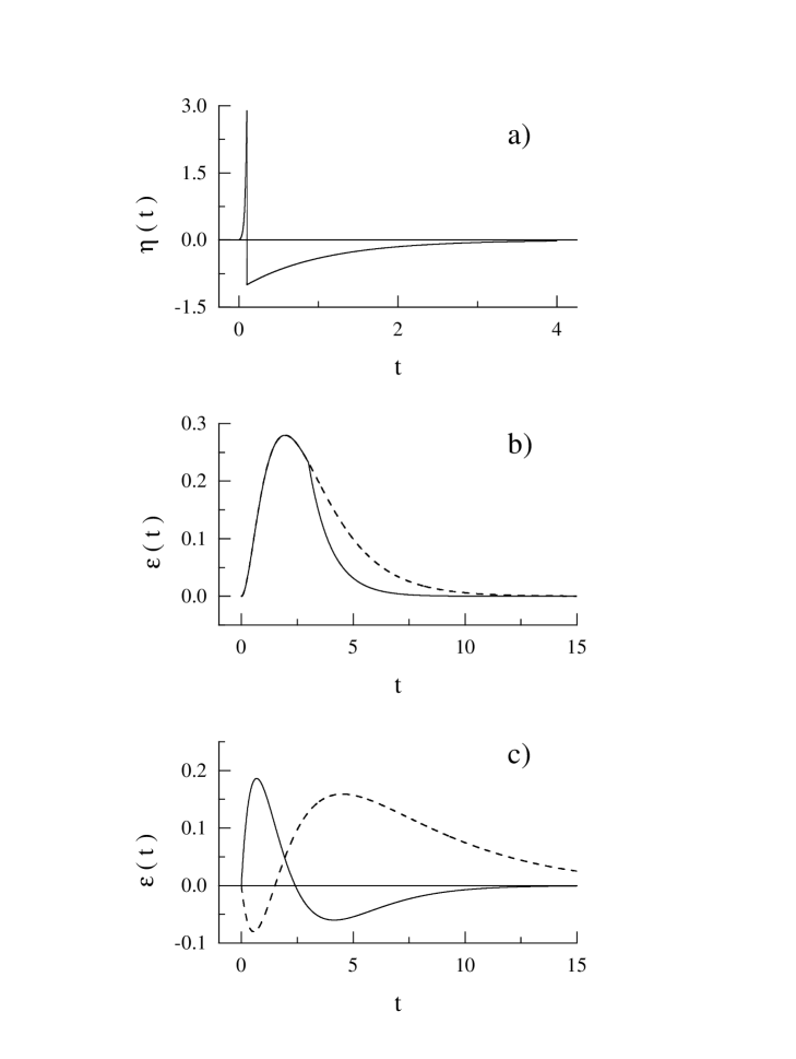
FIG. 2.: Example kernels. An $\eta$ kernel with a spike is shown in a). The kernel for the integrate-and-fire model would be identical without the spike. In b) we show the $\epsilon$ kernel from Eq. (7) for the saturating case (solid line) and the nonsaturating case (dashed line). Two examples of kernels for Type II neurons are shown in c). Note that they have both positive and negative parts.

FIG. 3.: Two examples of $G(\phi)$ for various values of $\alpha$, $\beta$, and $T$. The intersection of $G(\phi)$ and the horizontal line given by $I_{1}-I_{2}$ gives a phase-locked solution. If $|I_{1}-I_{2}|$ is large enough then no phase-locked solution exists.

REFERENCES

- [1] R. Llinás and U. Ribary Coherent 40-Hz oscillation characterizes dream state in humans. Proc. Natl. Acad. Sci. USA 90, 2078-2081 (1993).
- [2] C.M. Gray. Synchronous oscillations in neuronal systems: mechanisms and functions. J. Comp. Neurosci. 1, 11-38 (1994).
- [3] M.A. Whittington, R.D. Traub, and J.G.R. Jefferys. Synchronized oscillations in interneuron networks driven by metabotropic glutamate receptor activation. Nature 373, 612-615 (1995).
- [4] J.G.R. Jeffreys, R.D. Traub, and M.A. Whittington. Neuronal networks for induced ‘40 Hz’ rhythms. Trends Neurosci. 19, 202-207 (1996).
- [5] R.D. Traub, M.A. Whittington, S. Colling, G. Buzsáki, and J.G.R. Jefferys. Analysis of gamma rhythms in the rat hippocampus in vitro and in vivo. J. Physiol. 493, 471-484 (1996).
- [6] A.T. Winfree. Biological rhythms and the behavior of populations of coupled oscillators. J. Theoret. Biol. 16, 15-42 (1967).
- [7] S. Strogatz. Norbert Wiener’s brain waves. Lecture notes in biomathematics 100 (1993).
- [8] A.V.M. Herz and J.J. Hopfield. Earthquake cycles and neural reverberations: collective oscillations in systems with pulse-coupled threshold elements. Phys. Rev. Lett. 75, 1222-1225 (1995).
- [9] R. Mirollo and S. Strogatz. Synchronization of pulse-coupled biological oscillators. SIAM J. Appl. Math. 50, 1645-1662 (1990).
- [10] C. van Vreeswijk, L. Abbott, and G.B. Ermentrout. When inhibition not excitation synchronizes neural firing. J. Comp. Neuroscience 1, 313-321 (1994).
- [11] D. Hansel, G. Mato, and C. Meunier. Synchrony in excitatory neural networks. Neural Comp. 7, 307-337 (1995).
- [12] W. Gerstner, J.L. van Hemmen, and J. Cowen. What matters in neuronal locking? Neural Computation 8 1653-1676 (1996).
- [13] S. Bottani. Pulse-coupled relaxation oscillators: from biological synchronization to self-organized criticality. Phys. Rev. Lett. 74, 4189-4192 (1995).
- [14] U. Ernst, K. Pawelzik, and T. Geisel. Synchronization induced by temporal delays in pulse-coupled oscillators. Phys. Rev. Lett. 74, 1570-1573 (1995).
- [15] C. van Vreeswijk. Partial Synchronization in populations of pulse-coupled oscillators, Phys. Rev. E 54, 5522-5537 (1996).
- [16] Y. Kuramoto, in International Symposium on Mathematical Problems in Theoretical Physics. H. Araki, ed. Lecture Notes in Physics 39 (Springer, New York, 1975).
- [17] S. Strogatz and R. Mirollo. Collective synchronisation in lattices of non-linear oscillators with randomness. J. Phys. A.: Math. Gen. 21, L699-L705 (1988).
- [18] D. Golomb and J. Rinzel. Dynamics of globally coupled inhibitory neurons with heterogeneity. Phys. Rev. E 48, 4810-4814 (1993).
- [19] M. Tsodyks, I. Mitkov, and H. Sompolinsky, Phys. Rev. Lett. 71, 1280-1283 (1993).
- [20] X.-J. Wang and G. Buzsáki. Gamma oscillation by synaptic inhibition in an interneuronal network model. J. Neurosci. 16, 6402-6413 (1996).
- [21] J.A. White, C.C. Chow, J. Ritt, C. Soto-Trevino, and N. Kopell. J. Comp. Neurosci. (in press).
- [22] D. Terman, N. Kopell, and A. Bose. Dynamics of two neurons coupled by mutual slow inhibition. Preprint (1997).
- [23] G.B. Ermentrout. Type I membranes, phase resetting curves, and synchrony. Neural Comp. 8, 979-1001 (1996).
- [24] J. Rinzel and G.B. Ermentrout, in Methods in Neuronal Modelling, edited by C. Koch and I. Segev (MIT Press, Cambridge, 1989).
- [25] W. Gerstner and J.L. van Hemmen. Network 3, 139-164 (1992).
- [26] W. Gerstner. Time structure of the activity in neural network models. Phys. Rev. E 51, 738-758 (1995).
- [27] W. Kistler, W. Gerstner, and J. L van Hemmen. Reduction of the Hodgkin-Huxley Equations to a Single-Variable Threshold Model. Neural Computation 9, 1069-1100 (1997).
- [28] C. Chow, J.A. White, J. Ritt, and N. Kopell. Frequency control in synchronous networks of inhibitory neurons. unpublished (1997).
- [29] L. Abbott and C. van Vreeswijk. Asynchronous states in networks of pulse-coupled oscillators. Phys. Rev. E 48, 1483-1490 (1993).
- [30] H. Tuckwell. Stochastic processes in the neurosciences. (SIAM, Philadelphia, 1989).
- [31] D.G. Aronson, M. Golubitsky, and J. Mallet-Paret. Ponies on a merry-go-round in large arrays of Josephson junctions. Nonlinearity 4, 903-910 (1991).
- [32] J.W. Swift, S.H. Strogatz, and K. Wiesenfeld. Averaging of globally coupled oscillators. Physica D 55, 239-250 (1992).
- [33] S.H. Strogatz and R.E. Mirollo. Splay states in globally coupled Josephson arrays: analytical prediction of Floquet multipliers. Phys. Rev. E 47, 220-227 (1993).
- [34] I.B. Schwartz and K.Y. Tsang. Antiphase switching in Josephson junction arrays. Phys. Rev. Lett. 73, 2797-2800 (1994).
- [35] C. Peskin. Mathematical Aspects of Heart Physiology (Courant Institute of Mathematical Sciences, New York University, New York, 1975) p. 268-278.
- [36] G.B. Ermentrout and N. Kopell. Frequency plateaus in a chain of weakly coupled oscillators. SIAM J. Math. Anal. 15, 215-237 (1984).
- [37] Y. Kuramoto. Chemical Oscillations, Waves and Turbulence. (Springer, Berlin, 1984).
- [38] L. Abbott. A network of oscillators. J. Phys. A 23 3835 (1990).
- [39] X.-J. Wang and J. Rinzel. Alternating and synchronous rhythms in reciprocally inhibitory model neurons. Neural Communication 4, (1992).
- [40] R.A. Horn and C.A. Johnson. Matrix Analysis, (Cambridge University Press, Cambridge, 1985).
- [41] P. Pinsky. SIAM J. Appl. Math. 55, 220–241 (1995).
- [42] A. Treves. Mean-field analysis of neuronal spike dynamics. Network 4, 259-284 (1993).
- [43] D. Golomb, D. Hansel, B. Shraiman, and H. Sompolinsky. Phys. Rev. A 45, 3516 (1992).
- [44] D. Golomb and J. Rinzel. Clustering in globally coupled inhibitory neurons. Physica D 72, 259-282 (1994).
- [45] N. Kopell and G. Le Masson. Rhythmogenesis, amplitude modulation and multiplexing in a cortical architecture. Proc. Nat. acad. Sci (USA) 91, 10586-19590 (1994).