Stability of the replica symmetric solution for the information conveyed by a neural network

Abstract

The information that a pattern of firing in the output layer of a feedforward network of threshold-linear neurons conveys about the network’s inputs is considered. A replica-symmetric solution is found to be stable for all but small amounts of noise. The region of instability depends on the contribution of the threshold and the sparseness: for distributed pattern distributions, the unstable region extends to higher noise variances than for very sparse distributions, for which it is almost nonexistant.

I Introduction

Advances in techniques for the formal analysis of neural networks [1, 2, 3, 4, 5] offer insight into the behaviour of models of biological interest. Of particular interest are methods which allow the calculation of the information that can be conveyed by a given neural structure, as these offer both useful intuitions and the prospect of conducting pertinent experiments[6]. The replica trick [7] has been used to achieve this in the case of binary units [5] and threshold-linear units [8, 9], by appealing to an assumption of replica symmetry. In the case of binary units with continuous inputs, the validity of the replica-symmetric ansatz is justified by the duality with the Gardner calculation of the storage capacity for continuous couplings [2, 5, 10]. We now analyse the stability of the replica symmetric solution for mutual information in a network of threshold-linear units.

The model describes a feedforward network of threshold-linear units with partially diluted connectivity. This is a simpler version of the calculation described in [8, 9]. In the calculation considered here, there is only one mode of operation (which we might call “transmission”), as opposed to the division into storage and recall modes in that calculation. There are $N$ cells in the input layer, and $M$ (proportional to $N$) in the output layer. The limit of interest is $N\to\infty$.

$\{\eta_{i}\}$ are the firing rates of each cell $i$ in the input layer. The probability density of finding a given firing pattern is taken to be:

$$P(\{\eta_{i}\})\prod_{i}d\eta_{i}=\prod_{i}P_{\eta}(\eta_{i})d\eta_{i}$$ (1)

Each input cell is thus assumed to code independent information.

$\{\xi_{j}\}$ are the firing rates produced in each cell in the output layer. They are determined by the matrix multiplication of the pattern $\{\eta_{i}\}$ with the synaptic weights $J_{ij}$, followed by Gaussian distortion, thresholding and rectification.

$$\xi_{j}=\left[\xi_{0}+\sum_{i}c_{ij}J_{ij}\eta_{i}+\epsilon_{j}\right]^{+}=\left[{\tilde{\xi}}_{j}\right]^{+}$$ (2)

$$\left<(\epsilon_{j})^{2}\right>=\sigma^{2}_{\epsilon}\\$$ (3)

Each output cell receives $C_{j}$ (which we will take to be of the order of $10^{4}$) connections from input layer cells:

$$c_{ij}\in\{0,1\}\qquad\left<c_{ij}\right>N=C_{j}\qquad(C\equiv\left<C_{j}\right>)$$ (4)

The mean value across all patterns of each synaptic weight is taken to be equal across synapses, and is therefore taken into the threshold term. The synaptic weights $J_{ij}$ are thus of zero mean, and variance $\sigma^{2}_{J}$ (all that affects the calculation is the first two moments of their distribution).

$$\left<(J_{ij})^{2}\right>=\sigma^{2}_{J}.$$ (5)

The average of the mutual information

$$I(\{\eta_{i}\},\{\xi_{j}\})=\int\prod_{i}d\eta_{i}\int\prod_{j}d\xi_{j}P(\{\eta_{i}\},\{\xi_{j}\})\ln{P(\{\eta_{i}\},\{\xi_{j}\})\over P(\{\eta_{i}\})P(\{\xi_{j}\})}$$ (6)

over the quenched variables $c_{ij},J_{ij}$ is written using the replica trick as

$$\left<I(\eta,\xi)\right>_{c,J}=\lim_{n\to 0}{1\over n}\left<\int d\eta d\xi P(\eta,\xi)\left\{\left[P(\eta,\xi)\over P(\eta)\right]^{n}-\left[P(\xi)\right]^{n}\right\}\right>_{c,J}.$$ (7)

The calculation is valid only for non-zero noise variance, and it will be seen that the only region in which the solution is not well behaved is that of very low noise variance.

II Calculation of mutual information

First, introducing replica indices $\alpha=1,..,n+1$, and breaking the integral over $\xi$ into subthreshold and suprathreshold components, we observe that

$$\left<I(\eta,\xi)\right>_{c,J} = \lim_{n\to 0}\frac{1}{n}\Bigg{\{}\int d\eta\left[\frac{1}{P(\eta)}\right]^{n}\prod_{\alpha}\left(\int_{-\infty}^{0}d{\tilde{\xi}}^{\alpha}\left<P(\eta^{\alpha},{\tilde{\xi}}^{\alpha})|_{\eta^{\alpha}=\eta}\right>_{c,J}\right)$$ (11)

$$+\int d\eta\left[\frac{1}{P(\eta)}\right]^{n}\int_{0}^{\infty}d{\tilde{\xi}}\prod_{\alpha}\left<P(\eta^{\alpha},{\tilde{\xi}}^{\alpha})|_{\eta^{\alpha}=\eta,{\tilde{\xi}}^{\alpha}={\tilde{\xi}}}\right>_{c,J}$$

$$-\prod_{\alpha}\left(\int_{-\infty}^{0}d{\tilde{\xi}}^{\alpha}\int d\eta^{\alpha}\left<P(\eta^{\alpha},{\tilde{\xi}}^{\alpha})\right>_{c,J}\right)$$

$$-\int_{0}^{\infty}d{\tilde{\xi}}\prod_{\alpha}\left(\int d\eta^{\alpha}\left<P(\eta^{\alpha},{\tilde{\xi}}^{\alpha})|_{{\tilde{\xi}}^{\alpha}={\tilde{\xi}}}\right>_{c,J}\right)\Bigg{\}}$$

This allows us to treat both terms of Eq. 7 in the same manner. To obtain the probability density $\left<P(\eta^{\alpha},{\tilde{\xi}}^{\alpha})\right>$, we use Dirac delta functions to implement the constraints defined by (2):

$$\left<P(\eta^{\alpha},{\tilde{\xi}}^{\alpha})\right>_{c,J} = \Bigg{<}\int\left[\prod_{j}D\left(\frac{\epsilon_{j}^{\alpha}}{\sigma_{\epsilon}}\right)\right]\left[\prod_{ij}D\left(\frac{J_{ij}}{\sigma_{J}}\right)\right]\prod_{j}\delta\left[{\tilde{\xi}}_{j}^{\alpha}-\xi_{0}-\sum_{i}c_{ij}J_{ij}\eta_{i}^{\alpha}-\epsilon_{j}^{\alpha}\right]$$ (13)

$$\times P(\{\eta_{i}^{\alpha}\})^{n+1}\Bigg{>}_{c}$$

where

$$Du=\frac{du}{\sqrt{2\pi}}e^{-u^{2}/2}$$ (14)

Using the integral form of the Dirac delta function introduces a Lagrange multiplier $x_{j}^{\alpha}$. The integrals over the noise and interaction distributions are performed, and the quenched average over the connections performed in the thermodynamic limit, so that

$$\left<P(\eta,{\tilde{\xi}})^{n+1}\right> = \int(\prod_{j\alpha}\frac{dx_{j}^{\alpha}}{2\pi})\exp\left\{i\sum_{j\alpha}x_{j}^{\alpha}({\tilde{\xi}}_{j}^{\alpha}-\xi_{0})\right.$$ (16)

$$\left.-\frac{1}{2}\sum_{j\alpha\beta}x_{j}^{\alpha}x_{j}^{\beta}\left[\sigma_{\epsilon}^{2}\delta_{\alpha\beta}+\frac{\sigma_{J}^{2}C}{N}\sum_{i}\eta_{i}^{\alpha}\eta_{i}^{\beta}\right]P(\{\eta_{i}^{\alpha}\})^{n+1}\right\}$$

where $\delta_{\alpha\beta}$ is the Kronecker delta. A Lagrange multiplier

$$z^{\alpha\beta}=\frac{1}{N}\sum_{i}\eta_{i}^{\alpha}\eta_{i}^{\beta}$$ (17)

is introduced using the integral form of the Dirac delta function via an auxiliary variable $\tilde{z}^{\alpha\beta}$. We then obtain

$$\left<P(\eta,{\tilde{\xi}})^{n+1}\right> = \int(\prod_{\alpha}\frac{dz^{\alpha}d\tilde{z}^{\alpha}}{2\pi/N})(\prod_{(\alpha\beta)}\frac{dz^{\alpha\beta}d\tilde{z}^{\alpha\beta}}{2\pi/N})\exp\Bigg{\{}iN\sum_{\alpha}z^{\alpha}{\tilde{z}}^{\alpha}+iN\sum_{(\alpha\beta)}z^{\alpha\beta}{\tilde{z}}^{\alpha\beta}$$ (18)

$$- \left.\sum_{\alpha}{\tilde{z}}^{\alpha}\sum_{i}(\eta_{i}^{\alpha})^{2}-\sum_{(\alpha\beta)}{\tilde{z}}^{\alpha\beta}\sum_{i}\eta_{i}^{\alpha}\eta_{i}^{\beta}-\frac{1}{2}\sum_{j\alpha\beta}({\tilde{\xi}}_{j}^{\alpha}-\xi_{0})E_{\alpha\beta}({\tilde{\xi}}_{j}^{\beta}-\xi_{0})\right.$$ (19)

$$- \frac{1}{2}{\rm{Tr}}\ln{\mathbf{M}}\Bigg{\}}(2\pi)^{-\frac{n+1}{2}}P(\{\eta_{i}^{\alpha}\})^{n+1}$$ (20)

where $\mathbf{M}=\sigma_{\epsilon}^{2}\mathbf{I}+\sigma_{J}^{2}\mathnormal{C}\mathbf{Z}$ and $\mathbf{E}={\mathbf{M}}^{-1}$. $\mathbf{Z}$ is the matrix with elements $z^{\alpha\beta}$, and $(\alpha\beta)$ is the pair $\alpha\beta$, $\alpha\neq\beta$.

Thus

$$\left<I\right>=\lim_{n\to 0}\Bigg{\{}\int(\prod_{\alpha}\frac{dz^{\alpha}d{\tilde{z}}^{\alpha}}{2\pi/N})\exp\left[iN\sum_{\alpha}z^{\alpha}{\tilde{z}}^{\alpha}-N{\mathcal{H}}_{A}({\tilde{z}}^{\alpha})-M{\mathcal{G}}(z^{\alpha},z^{\alpha})\right]$$ (21)

$$-\int(\prod_{\alpha}\frac{dz^{\alpha}d{\tilde{z}}^{\alpha}}{2\pi/N})(\prod_{(\alpha\beta)}\frac{dz^{\alpha\beta}d{\tilde{z}}^{\alpha\beta}}{2\pi/N})\exp\Bigg{[}iN\sum_{\alpha}z^{\alpha}{\tilde{z}}^{\alpha}+iN\sum_{(\alpha\beta)}z^{\alpha\beta}{\tilde{z}}^{\alpha\beta}$$ (22)

$$-N{\mathcal{H}}_{B}({\tilde{z}}^{\alpha},{\tilde{z}}^{\alpha\beta})-M{\mathcal{G}}(z^{\alpha},z^{\alpha\beta})\Bigg{]}\Bigg{\}}$$ (23)

where

$${e^{-{\mathcal{H}}_{A}}}({\tilde{z}}^{\alpha})=\int_{\eta}d\eta P(\eta)\exp\left(-\sum_{\alpha}{\tilde{z}}^{\alpha}\eta^{2}\right)\\$$ (24)

$${e^{-{\mathcal{H}}_{B}}}({\tilde{z}}^{\alpha},{\tilde{z}}^{\alpha\beta})=\int_{\eta}(\prod_{\alpha}d\eta^{\alpha}P(\eta^{\alpha}))\exp{\left(-\sum_{\alpha}{\tilde{z}}^{\alpha}(\eta^{\alpha})^{2}-\sum_{(\alpha\beta)}{\tilde{z}}^{\alpha\beta}\eta^{\alpha}\eta^{\beta}\right)}\\$$ (25)

$${e^{-\mathcal{G}}}(z^{\alpha},z^{\alpha\beta}) = e^{-\frac{1}{2}\mathrm{Tr}\ln{\mathbf{M}}}\Bigg{\{}\int_{0}^{\infty}\frac{d{\tilde{\xi}}}{\sqrt{2\pi}}\exp{-\frac{1}{2}({\tilde{\xi}}-\xi_{0})^{2}\sum_{\alpha\beta}E_{\alpha\beta}}$$ (26)

$$+ \int_{-\infty}^{0}(\prod_{\alpha}\frac{d{\tilde{\xi}}^{\alpha}}{\sqrt{2\pi}})\exp\left[-\frac{1}{2}\sum_{\alpha\beta}({\tilde{\xi}}^{\alpha}-\xi_{0})E_{\alpha\beta}({\tilde{\xi}}^{\beta}-\xi_{0})\right]\Bigg{\}}$$ (27)

III Replica symmetric solution

The assumption of replica symmetry can be written

$$z_{A}^{\alpha}=z_{A}^{\alpha\beta} = z_{0A}(n)\qquad i{\tilde{z}}_{A}^{\alpha}={\tilde{z}}_{0A}(n)$$ (28)

$$z_{B}^{\alpha} = z_{0B}(n)\qquad i{\tilde{z}}_{B}^{\alpha}={\tilde{z}}_{0B}(n)$$ (29)

$$z_{B}^{\alpha\beta} = z_{1}(n)\qquad i{\tilde{z}}_{B}^{\alpha\beta}=-{\tilde{z}}_{1}(n)$$ (30)

The saddle-point method is utilized in the thermodynamic limit, yielding the saddle-point equations

$$z_{0A}=\left<\eta^{2}\right>_{\eta}$$ (33)

$${\tilde{z}}_{0A}=0$$ (34)

$$z_{0B}=\left<\eta^{2}\right>_{\eta}$$ (35)

$${\tilde{z}}_{0B}=0$$ (36)

$$z_{1}=-\int_{-\infty}^{\infty}Ds\left<(\eta^{2}+\frac{s\eta}{\sqrt{{\tilde{z}}_{1}}})\exp(-\frac{{\tilde{z}}_{1}}{2}\eta^{2}-s\sqrt{{\tilde{z}}_{1}}\eta)\right>_{\eta}\ln\left<\exp(-\frac{{\tilde{z}}_{1}}{2}\eta^{2}-s\sqrt{{\tilde{z}}_{1}}\eta)\right>_{\eta}$$ (37)

$${\tilde{z}}_{1} = -\sigma_{J}^{2}Cr\Bigg{\{}\frac{\xi_{0}}{(p_{B}+q_{B})^{3/2}}\sigma(\frac{\xi_{0}}{\sqrt{p_{B}+q_{B}}})-\frac{1}{p_{B}}\phi\left(\frac{\xi_{0}}{\sqrt{p_{B}+q_{B}}}\right)$$ (38)

$$+ \int_{-\infty}^{\infty}Dt\left[1+\ln\phi\left(\frac{-\xi_{0}-t\sqrt{q_{B}}}{\sqrt{p_{B}}}\right)\right]\sigma\left(\frac{-\xi_{0}-t\sqrt{q_{B}}}{\sqrt{p_{B}}}\right)p_{B}^{-3/2}\left(\xi_{0}+\frac{t(p_{B}+q_{B})}{\sqrt{q_{B}}}\right)\Bigg{\}}$$ (39)

and the expression for the information per input cell

$$\left<i\right>= r G(p_{A},q_{A})+\frac{1}{2}z_{1}{\tilde{z}}_{1}-rG(p_{B},q_{B})$$ (40)

$$- \int_{-\infty}^{\infty}Ds\left<\exp(-\frac{1}{2}{\tilde{z}}_{1}\eta^{2}-s\sqrt{{\tilde{z}}_{1}}\eta)\right>_{\eta}\ln\left<\exp(-\frac{1}{2}{\tilde{z}}_{1}\eta^{2}-s\sqrt{{\tilde{z}}_{1}}\eta)\right>_{\eta}$$ (41)

where

$$G(p,q)=\frac{p\xi_{0}}{2(p+q)^{3/2}}\sigma\left(\frac{\xi_{0}}{\sqrt{p+q}}\right)-\frac{1}{2}(1+\ln{p}){\phi\left(\frac{\xi_{0}}{\sqrt{p+q}}\right)}$$ (42)

$$+\int_{-\infty}^{\infty}Dt\phi\left(\frac{-\xi_{0}-t\sqrt{q}}{\sqrt{p}}\right)\ln\phi\left(\frac{-\xi_{0}-t\sqrt{q}}{\sqrt{p}}\right)$$ (43)

and

$$\left<x(\eta)\right>_{\eta} = \int_{\eta}d\eta P(\eta)x(\eta)$$ (44)

$$\phi(x) = \int_{-\infty}^{x}Ds$$ (45)

$$\sigma(x) = \frac{1}{\sqrt{2\pi}}e^{-x^{2}/2}$$ (46)

$$p_{A} = \sigma_{\epsilon}^{2}\qquad\qquad p_{B}=\sigma_{\epsilon}^{2}+\sigma_{J}^{2}C(z_{0B}-z_{1})$$ (48)

$$q_{A} = \sigma_{J}^{2}Cz_{0A}\qquad q_{B}=\sigma_{J}^{2}Cz_{1}.$$ (49)

We refer to $r=M/N$ as the anatomical divergence.

This expression must in general be evaluated numerically. However, considering some limiting cases can give us some insight into the behaviour of the solution. In particular, the limit of linear processing can be obtained by taking $\xi_{0}\to+\infty$. In this limit, Eq. 39 reduces to

$${\tilde{z}}_{1}\to\frac{\sigma_{J}^{2}Cr}{p_{B}}.$$ (51)

The information per neuron obtained in the linear limit is

$$\left<i\right>\to \frac{1}{2}r\ln\frac{p_{B}}{p_{A}}+\frac{1}{2}z_{1}{\tilde{z}}_{1}$$ (52)

$$- \int_{-\infty}^{\infty}Ds\left<\exp(-\frac{1}{2}{\tilde{z}}_{1}\eta^{2}-s\sqrt{{\tilde{z}}_{1}}\eta)\right>_{\eta}\ln\left<\exp(-\frac{1}{2}{\tilde{z}}_{1}\eta^{2}-s\sqrt{{\tilde{z}}_{1}}\eta)\right>_{\eta}.$$ (53)

The information obtained in this limit is bounded by that which would be obtained from a simple Gaussian channel calculation, where we consider the channel

$$\xi_{j}^{*}=\sum_{i}c_{ij}J_{ij}\eta_{i}+\epsilon_{j},$$ (54)

and perform the annealed and quenched averages to obtain the signal variance $\sigma_{J}^{2}C(\left<\eta^{2}\right>_{\eta}-\left<\eta\right>_{\eta}^{2})$, and information per input cell

$$I_{gauss}=\frac{r}{2}\ln\left[1+\frac{\sigma_{J}^{2}C(\left<\eta^{2}\right>_{\eta}-\left<\eta\right>_{\eta}^{2})}{\sigma_{\epsilon}^{2}}\right].$$ (55)

The Gaussian channel information provides an upper limit corresponding to the optimal $\eta$ distribution (for transmitting maximal information given a constraint on the signal power), and no dependence upon the same inputs of the output cells.

Within the linear limit, we can consider the special case of high noise variance (low signal to noise ratio). As $\sigma_{\epsilon}^{2}\to\infty$,

$${\tilde{z}}_{1}\sim\frac{\sigma_{J}^{2}Cr}{\sigma_{\epsilon}^{2}},$$ (56)

and

$$z_{1}\simeq\left<\eta\right>^{2}+O({\tilde{z}}_{1}).$$ (57)

The information therefore falls to zero as

$$\left<i\right>\sim\frac{\sigma_{J}^{2}Cr(\left<\eta^{2}\right>_{\eta}-\left<\eta\right>_{\eta}^{2})}{2\sigma_{\epsilon}^{2}},$$ (58)

i.e. inversely with noise variance, as one would expect. We thus can see that for linear neurons with low signal to noise ratio, the transmitted information approaches the Gaussian channel limit.

The numerical solution of the mutual information expression, as a function of the noise variance, is shown in Fig. 1, both for the case of linear units and for units with a threshold of $\xi_{0}=-0.4$, representing threshold-linear behaviour. This is shown for a binary pattern distribution of sparseness $a$, where the sparseness of a distribution is a mean-invariant measure of spread and is defined in general as

$$a=\frac{\left<\eta\right>_{\eta}^{2}}{\left<\eta^{2}\right>_{\eta}}.$$ (59)

This measure is ‘more sparse’ for smaller $a$, and reduces to the fraction of units ‘on’ in the case of a binary distribution. The Gaussian channel bound appears on the same graphs for comparison.

The mutual information should be bounded by the pattern entropy as the noise variance becomes very small. As the noise variance decreases, the replica-symmetric solution approaches this bound in both the linear and threshold-linear cases. It can be seen, however, that for very small noise variances, the replica-symmetric solution changes direction and crosses this physical boundary. Inspection of Eq. 43 reveals divergence of the mutual information solution in the limit $\sigma_{\epsilon}^{2}\to 0$; this is in keeping with our intuition from the beginning that the calculation should not be valid in the deterministic limit. However, for such low noise variance the information has essentially saturated in any case. For threshold-linear neurons, the solution is also unstable to replica-symmetry-breaking fluctuations for relatively low noise variance, as will be discussed in the next section.

IV Stability of the replica-symmetric solution

The stability of the replica-symmetric solution is analysed after the style of de Almeida-Thouless [11]. For the solution for free energy this was addressed in the context of Hopfield-Little type autoassociative neural networks in [1], and for an autoassociator with threshold-linear units and for a threshold-linear variant of the Sherrington-Kirkpatrick model in [12]. For the solution for another quantity, the Gardner volume, this was addressed in [2] for Ising ($\pm 1$) neurons. In contrast, here we are determining the stability of the solution for mutual information in a network comprised of threshold-linear neurons, although the technique proceeds very similarly.

Fluctuations in the transverse (replica-symmetry breaking, RSB) and longitudinal (replica-symmetric, RS) directions are decoupled, and hence can be analysed separately. Longitudinal fluctuations can be disregarded [11, 13] if a unique saddle-point is obtained, which appears to be the case. We will therefore concentrate upon transverse fluctuations.

We wish to consider small deviations in the saddle-point parameters about the replica-symmetric saddle-point,

$$z^{\alpha\beta}=z_{1}+\delta z^{\alpha\beta}$$ (60)

$${\tilde{z}}^{\alpha\beta}={\tilde{z}}_{1}+\delta{\tilde{z}}^{\alpha\beta}$$ (61)

Quadratic fluctuations in the function

$${\mathcal{B}}(z^{\alpha},{\tilde{z}}^{\alpha},z^{\alpha\beta},{\tilde{z}}^{\alpha\beta})=iN\sum_{\alpha}z^{\alpha}{\tilde{z}}^{\alpha}+iN\sum_{(\alpha\beta)}z^{\alpha\beta}{\tilde{z}}^{\alpha\beta}\\ -N{\mathcal{H}}_{B}({\tilde{z}}^{\alpha},{\tilde{z}}^{\alpha\beta})-M{\mathcal{G}}(z^{\alpha},z^{\alpha\beta}).$$ (62)

give us the stability matrix

$$\mathbf{\Gamma}=\left[\matrix{\frac{\displaystyle\partial^{2}\mathcal{B}}{\displaystyle\partial z^{\alpha\beta}\partial z^{\gamma\delta}}&\frac{\displaystyle\partial^{2}\mathcal{B}}{\displaystyle\partial z^{\alpha\beta}\partial(i{\tilde{z}}^{\gamma\delta})}\cr\frac{\displaystyle\partial^{2}\mathcal{B}}{\displaystyle\partial(i{\tilde{z}}^{\alpha\beta})\partial z^{\gamma\delta}}&\frac{\displaystyle\partial^{2}\mathcal{B}}{\displaystyle\partial(i{\tilde{z}}^{\alpha\beta})\partial(i{\tilde{z}}^{\gamma\delta})}}\right]=\left[\matrix{A^{(\alpha\beta)(\gamma\delta)}&\delta_{(\alpha\beta)(\gamma\delta)}\cr\delta_{(\alpha\beta)(\gamma\delta)}&B^{(\alpha\beta)(\gamma\delta)}}\right]$$ (63)

where $\delta_{(\alpha\beta),(\gamma\delta)}=\delta_{\alpha\gamma}\delta_{\beta\delta}+\delta_{\alpha\delta}\delta_{\beta\gamma}$. In constrast to previous calculations based on quantities such as free energy, the expression for mutual information involves $n+1$ replicas. There are $n(n+1)/2$ independent variables $z^{\alpha\beta}$, and the same number of independent ${\tilde{z}}^{\alpha\beta}$. $\mathbf{\Gamma}$ is thus an $n(n+1)\times n(n+1)$ matrix.

The transverse eigenvalues of this matrix are given by the eigenvalues of the matrix

$$\left(\matrix{\lambda_{A}&1\cr 1&\lambda_{B}}\right),$$ (64)

where $\lambda_{A}$ and $\lambda_{B}$ are the transverse eigenvalues of the submatrices $A^{(\alpha\beta)(\gamma\delta)}$ and $B^{(\alpha\beta)(\gamma\delta)}$ respectively. Calculation of these involves consideration of the symmetry properties of the submatrices, and is detailed in the Appendix. The eigenvalue equations reduce to

$$\lambda_{A} +c=\lambda$$ (65)

$$1 +c\lambda_{B}=c\lambda$$ (66)

We thus have the two replicon mode eigenvalues

$$\lambda_{\pm}=\frac{1}{2}(\lambda_{A}+\lambda_{B})\pm\sqrt{\frac{1}{4}(\lambda_{A}-\lambda_{B})^{2}+1}$$ (67)

For stability, the product of the eigenvalues must be non-negative. A further subtlety is introduced here. $\lambda_{+}$ can be seen to be $>0$ irrespective of $\sigma_{\epsilon}^{2}$ or $a$. $\lambda_{-}$, on the other hand, changes sign, moving from negative to positive for smaller $\sigma_{\epsilon}^{2}$. However, intuitively we expect, from the analogy of the noise with the ‘temperature’ parameter in other models of neural networks[1] and physical systems[14] that if replica-symmetry breaking is to set in, it will do so at low noise variances. This is confirmed by the eminently sensible behaviour of the mutual information curves of Fig. 1 at medium to high noise, but nonphysical behaviour at very low noise values. It can be concluded that, as occurs in [1, 12], a sign reversal has been introduced due to the integration contour, which must be corrected.

These equations have been numerically solved for $\lambda_{-}$. Fig. 2 shows the behavior of $\lambda_{-}$ for a range of sparsenesses and thresholds. Where the eigenvalue passes above the zero axis (dotted line), a phase of RS-instability is indicated. Fig. 2a is for the situation of quite sparse coding of the patterns. As the noise is reduced from the high noise region, in which the RS solution is stable, the eigenvalue changes sign, and an unstable region is entered. In the case of threshold $\xi_{0}$ = 0.4, which represents only a very small degree of threshold-like behavior, the eigenvalue can be seen to curve back and change sign again at lower noise values still. Due to non-convergence of numerical integration, it is not possible to examine extremely small noise values; therefore it is not clear from this diagram whether the eigenvalue also falls below zero again for the other curves plotted in this figure, or if it instead has a finite value at zero noise. However, any region of RS stability at noise variances this low would obviously be irrelevant for the same numerical reasons.

It is apparent from Figs. 2(b) and (c) that as the input distribution is made less sparse ($a$ is increased), the critical amount of noise below which instability arises increases. This will be discussed again shortly. Another effect that can be seen in Figs. 2(a) and (b) is that, as the neurons are made more linear ($\xi_{0}$ is increased), the critical noise first rises, then falls. This becomes more clear after plotting a phase diagram of noise against $\xi_{0}$ (Fig. 3). For low $a$ (sparse distributions), the critical noise rises, falls, and then curves back around on itself – after the neurons become sufficiently linear, there is no more region of instability. As the pattern code becomes less sparse, at first the region of instability merely expands. When $a$ reaches a certain value, however, the edge of the unstable region no longer curls in on itself, but extends outwards. At a sparseness of 0.5, for instance, the critical noise thus first rises with increasing linearity, taking longer to reach its peak than for more sparse distributions, then falls, and finally levels off and decreases slowly. The sparseness at which this change in behavior is exhibited is independent of the parameters of the system, and can be seen from Fig. 3 to lie somewhere between 0.2 and 0.5.

In the special case of the linear limit, in which $\xi_{0}\to\infty$, $\lambda_{A}$ disappears (see Appendix), and stability is assured. For finite $\xi_{0}$ and above the coefficient of sparseness referred to in the previous paragraph, though, there is a distinct and reasonably large region of instability.

The resulting phase diagrams are shown in Fig. 4. Fig. 4(a) shows the situation for $\xi_{0}=-0.4$, which corresponds to threshold-linear behavior. As $\xi_{0}$ is increased (Fig. 4b-d; the neurons are made progressively “more linear”), the critical noise variance at which instability of the RS solution sets in first increases, and then decreases, as would be expected from Fig. 3. In Fig. 4(d), the line of critical noise variance abruptly stops at $a\sim 0.23$: at this point, the replicon-mode eigenvalue passes below the zero axis, and stability is assured. In all cases, it is apparent that in particular for very sparse distributions, the replica-symmetric equations are valid down to quite low noise. For less sparse coding, where the pattern entropy is significantly higher, the replica-symmetry-broken solution would seem to be relevant for higher noise variances.

It should be noted that the sparseness of the distribution of outputs is not the same as that of the inputs. This can be determined by

$$a_{out}=\frac{\left<\xi\right>_{\xi^{+}}^{2}}{\left<\xi^{2}\right>_{\xi^{+}}}$$ (68)

where

$$\left<x(\xi)\right>_{\xi^{+}}=\int_{0}^{\infty}\frac{d\xi}{\sqrt{2\pi\sigma_{\xi}^{2}}}x(\xi)\exp-\frac{(\xi-\xi_{0})^{2}}{2\sigma_{\xi}^{2}}$$ (69)

$$\sigma_{\xi}^{2}=\sigma_{\epsilon}^{2}+\sigma_{J}^{2}C(\left<\eta^{2}\right>_{\eta}-\left<\eta\right>_{\eta}^{2}).$$ (70)

The lines of marginal stability for $\xi_{0}=-0.4$, $\xi_{0}=0.0$, $\xi_{0}=0.4$ and $\xi_{0}=0.80$ are replotted in Fig. 5 against the output sparseness. Although the phase diagrams look fairly similar when plotted as a function of input sparseness, they occupy different regions of the output sparseness domain because of the thresholding. It is also worth noting that because of the mapping performed by Eq. 68, the boundaries of the regions in Fig. 4 do not necessarily form the boundaries of the regions in the output-sparseness plane, which in some instances constitute points from inside the above curves.

For neurons operating in the threshold-linear regime (left curve, $\xi_{0}<0.0$), where output sparseness is effectively constrained by the thresholding, the stability characteristics are qualitatively as has been described earlier. For $\xi_{0}=0.0$, it is apparent from Eqs. 68 and 70 that the output sparseness is constant (regardless of the input sparseness) at a value of $1/\pi$. As $\xi_{0}$ is increased above zero, the output becomes less sparse, and the line of marginal stability is flipped horizontally (because in this range the entropy is higher for smaller $a_{out}$; right curves). Assuming that the sparseness of coding in connected sets of neurons in the brain tends to be similar, the former curve (for threshold-linear behaviour) might be considered the more biologically applicable, with the threshold in this model incorporating functionally the constraint on the degree of neural activity.

V Conclusions

This paper has detailed the replica symmetric solution for the information transmitted by a feedforward network of threshold-linear neurons, and examined its stability to fluctuations in the direction of replica symmetry breaking. It appears that for sparse pattern distributions, replica-symmetry breaking only sets in at noise variances sufficiently small that we might reasonably consider them to be ‘beyond the realm of biological interest’, at least for noisy cortical cells. We believe that, quite importantly, there is every reason to expect that these results carry over to the slightly more complicated ‘Schaffer collateral’ calculation described in [8, 9]. There is thus reason to feel confidence in the replica-symmetric assumption when analysing neural networks in areas such as the hippocampus which are known to code sparsely.

When more distributed (less sparse) encoding is used, the mutual information solution is prone to instability to replica-symmetry-breaking fluctuations at higher amounts of noise than in the sparse case. It is not clear from the current analysis what the quantitative effect of broken replica symmetry might be, or what the form of the exact solution would be in that case (e.g. the Parisi ansatz[15]). Care should therefore be taken when analysing the information conveyed by networks using more distributed encoding.

Appendix

In this appendix the transverse eigenvalues of the submatrices $A^{(\alpha\beta)(\gamma\delta)}$ and $B^{(\alpha\beta)(\gamma\delta)}$ are calculated. Both $A^{(\alpha\beta),(\gamma\delta)}$ and $B^{(\alpha\beta),(\gamma\delta)}$ have three different types of matrix elements depending on whether none, one or two replica indices of the pair $(\alpha\beta)$ equal those of the pair $(\gamma\delta)$. The three possible values $A^{(\alpha\beta),(\gamma\delta)}$ can take are:

$$P=\frac{\partial^{2}\mathcal{B}}{\partial z^{\alpha\beta}\partial z^{\alpha\beta}} = \frac{\sigma_{J}^{4}Cr}{4W}\frac{(q^{2}+2pq)^{2}}{p^{4}(p+q)^{4}}\Bigg{\{}\int_{0}^{\infty}\frac{d\xi}{\sqrt{2\pi}}(\xi-\xi_{0})^{4}\exp\left[-\frac{(\xi-\xi_{0})^{2}}{2(p+q)}\right]$$ (71)

$$+ \int_{-\infty}^{\infty}\frac{dt}{\sqrt{2\pi}}\bigg{[}(\xi-\xi_{0})^{2}\bigg{]}^{2}_{\xi^{-}}(\textstyle\frac{1}{2},t)\Bigg{\}}$$ (72)

$$Q=\frac{\partial^{2}\mathcal{B}}{\partial z^{\alpha\beta}\partial z^{\alpha\gamma}} = \frac{\sigma_{J}^{4}Cr}{4W}\frac{(q^{2}+2pq)^{2}}{p^{4}(p+q)^{4}}\Bigg{\{}\int_{0}^{\infty}\frac{d\xi}{\sqrt{2\pi}}(\xi-\xi_{0})^{4}\exp\left[-\frac{(\xi-\xi_{0})^{2}}{2(p+q)}\right]$$ (73)

$$+ \int_{-\infty}^{\infty}\frac{dt}{\sqrt{2\pi}}\bigg{[}(\xi-\xi_{0})^{2}\bigg{]}_{\xi^{-}}(\textstyle\frac{1}{3},t)\bigg{[}(\xi-\xi_{0})\bigg{]}^{2}_{\xi^{-}}(\textstyle\frac{1}{3},t)\Bigg{\}}\qquad(\beta\neq\gamma)$$ (74)

$$R=\frac{\partial^{2}\mathcal{B}}{\partial z^{\alpha\beta}\partial z^{\gamma\delta}} = \frac{\sigma_{J}^{4}Cr}{4W}\frac{(q^{2}+2pq)^{2}}{p^{4}(p+q)^{4}}\Bigg{\{}\int_{0}^{\infty}\frac{d\xi}{\sqrt{2\pi}}(\xi-\xi_{0})^{4}\exp\left[-\frac{(\xi-\xi_{0})^{2}}{2(p+q)}\right]$$ (75)

$$+ \int_{-\infty}^{\infty}\frac{dt}{\sqrt{2\pi}}\bigg{[}(\xi-\xi_{0})\bigg{]}^{4}_{\xi^{-}}(\textstyle\frac{1}{4},t)\Bigg{\}}\qquad(\alpha\neq\gamma,\beta\neq\delta),$$ (76)

where $\bigg{[}x(\xi)\bigg{]}_{\xi^{-}}(k,t)$ is defined as

$$\bigg{[}x(\xi)\bigg{]}_{\xi^{-}}(k,t)=\int_{-\infty}^{0}\frac{d\xi}{\sqrt{2\pi}}x(\xi)\exp\left[-\frac{k}{2p}(\xi-\xi_{0})^{2}+kt\sqrt{\frac{q}{p(p+q)}}(\xi-\xi_{0})-\frac{kt^{2}}{2}\right],$$ (78)

which can be considered to be a weighted average of $x(\xi)$ over the subthreshold values of $\xi$. $k$ is used to normalise the weight factor over the $t$ integral in each of Eqs. LABEL:eq:Apos. Also,

$$W=\phi\left(\frac{\xi_{0}}{\sqrt{p+q}}\right)+\int_{-\infty}^{\infty}\frac{dt}{\sqrt{2\pi}}\phi\left(-\frac{\xi_{0}}{\sqrt{p}}-t\sqrt{\frac{q}{p+q}}\right)\exp\left[-\frac{t^{2}(2p+q)}{4(p+q)}\right]\sqrt{p}.$$ (79)

and $p$,$q$ are here $p_{B}$ and $q_{B}$ from Eq. LABEL:eq:pq.

We have to solve the eigenvalue equation

$$\mathbf{A}\psi=\lambda\psi.$$ (80)

The eigenvectors $\psi$ have the column-vector form

$$\psi=\left(\{\delta z^{\alpha\beta}\}\ \right)\qquad(\alpha<\beta=1,..,n+1)$$ (81)

We now proceed as described in [11]. There are three classes of eigenvectors (and corresponding eigenvalues) – those invariant under interchange of all indices, those invariant under interchange of all but one index, and those invariant under interchange of all but two indices. These last describe the transverse mode, in which we are interested.

Let us consider fluctuations of the form

$$\delta z^{\alpha\beta} = \Delta^{\alpha\beta}\qquad(\alpha<\beta=1,..,n+1)$$ (82)

with

$$\Delta^{\alpha\beta}=\Delta\qquad\alpha,\beta\neq\alpha_{0},\beta_{0}$$ (84)

$$\Delta^{\alpha_{0}\beta}=\Delta^{\alpha\beta_{0}}=\frac{2-n}{2}\Delta\qquad\alpha\neq\alpha_{0},\beta_{0}$$ (85)

$$\Delta^{\alpha_{0}\beta_{0}}=\frac{(2-n)(1-n)}{2}\Delta$$ (86)

ensuring orthogonality between the eigenvectors describing RS and RSB fluctuations. As with [11], we have for $A^{(\alpha\beta),(\gamma\delta)}$ an eigenvalue

$$\lambda_{A}=P-2Q+R$$ (87)

with in this case $\frac{1}{2}(n+1)(n-2)$-fold degeneracy, and $P$, $Q$ and $R$ as described above.

For $B^{(\alpha\beta),(\gamma\delta)}$, we consider fluctuations

$$\delta{\tilde{z}}^{\alpha\beta} = c\Delta^{\alpha\beta}\qquad(\alpha<\beta=1,..,n+1)$$ (88)

and obtain similarly the eigenvalue

$$\lambda_{B}=P^{\prime}-2Q^{\prime}+R^{\prime},$$ (90)

where

$$P^{\prime} = \frac{\displaystyle\partial^{2}\mathcal{B}}{\displaystyle\partial(i{\tilde{z}}^{\alpha\beta})\partial(i{\tilde{z}}^{\alpha\beta})}=\int_{-\infty}^{\infty}Dt\bigg{[}\eta^{2}\bigg{]}^{2}_{\eta}(\textstyle\frac{1}{2},t)$$ (91)

$$Q^{\prime} = \frac{\displaystyle\partial^{2}\mathcal{B}}{\displaystyle\partial(i{\tilde{z}}^{\alpha\beta})\partial(i{\tilde{z}}^{\alpha\gamma})}=\int_{-\infty}^{\infty}Dt\bigg{[}\eta^{2}\bigg{]}_{\eta}(\textstyle\frac{1}{3},t)\bigg{[}\eta\bigg{]}^{2}_{\eta}(\textstyle\frac{1}{3},t)$$ (92)

$$R^{\prime} = \frac{\displaystyle\partial^{2}\mathcal{B}}{\displaystyle\partial(i{\tilde{z}}^{\alpha\beta})\partial(i{\tilde{z}}^{\gamma\delta})}=\int_{-\infty}^{\infty}Dt\bigg{[}\eta\bigg{]}^{4}_{\eta}(\textstyle\frac{1}{4},t),$$ (93)

and $\bigg{[}x(\eta)\bigg{]}_{\eta}(k,t)$, the weighted pattern average, is defined as

$$\bigg{[}x(\eta)\bigg{]}_{\eta}(k,t)=\int_{\eta}d\eta P(\eta)x(\eta)\exp\left[-\frac{k}{2}{\tilde{z}}_{1}\eta^{2}-kt\sqrt{{\tilde{z}}_{1}}\eta\right].$$ (95)

a

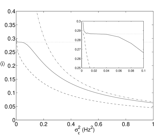
b

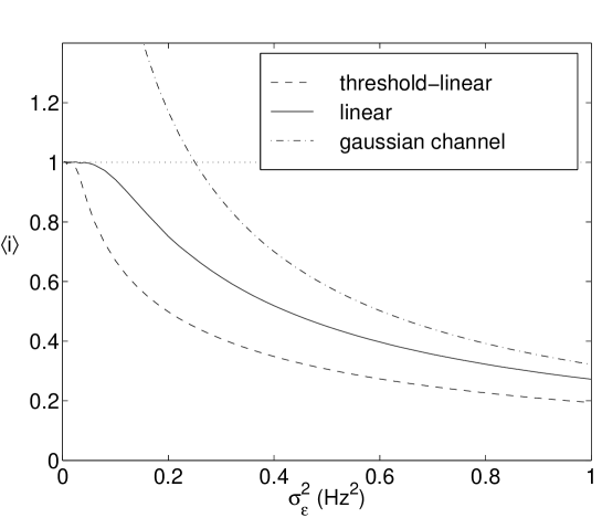
FIG. 1.: Mutual information, measured in bits, as a function of noise variance. The dashed line is for a threshold $\xi_{0}=-0.4$, whereas the solid line is for the limit of linear neurons. The dot-dashed line indicates the simple gaussian channel for comparison. The entropy of the input pattern distribution is indicated by the horizontal dotted line. (a) Input pattern distribution sparseness of 0.05. (b) Sparseness of 0.50.

a

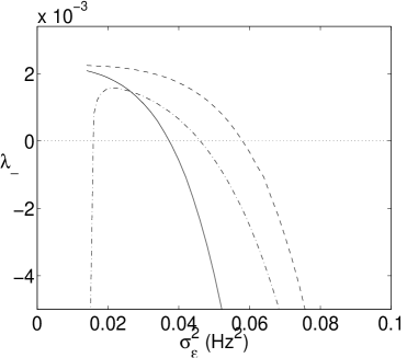
b

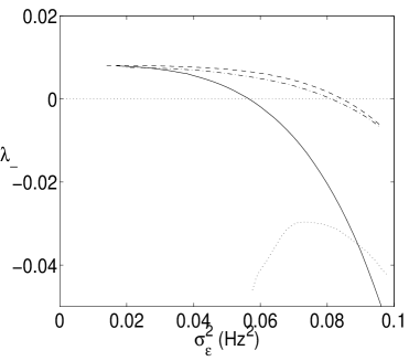
c

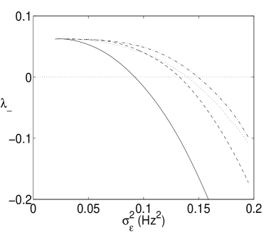
FIG. 2.: The behavior of the replicon mode eigenvalue $\lambda_{-}$ as a function of noise variance. (a) Input sparseness $a=0.05$ (b) $a=0.10$ (c) $a=0.50$. In each of these graphs the solid line indicates the eigenvalue for threshold $\xi_{0}=-0.4$, the dashed curve $\xi_{0}=0.0$, the dot-dashed curve $\xi_{0}=0.4$, and the dotted curve $\xi_{0}=0.8$. The replica symmetric solution is unstable in regions where these curves lie above the horizontal dotted line. In case (a), the $\xi_{0}=0.8$ line lies below the region examined in the graph.

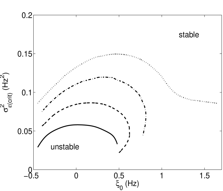
FIG. 3.: A phase diagram showing the critical noise variance as a function of the threshold parameter, $\xi_{0}$ – the larger $\xi_{0}$ is, the more linear the regime. Solid curve, sparseness $a=0.05$; dashed curve, $a=0.10$; dot-dashed curve, $a=0.20$; dotted curve, $a=0.50$.

a

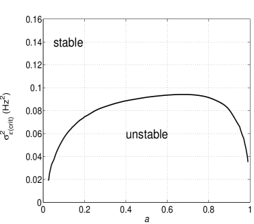
b

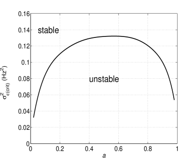
c

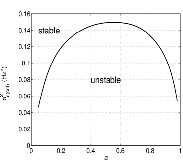
d

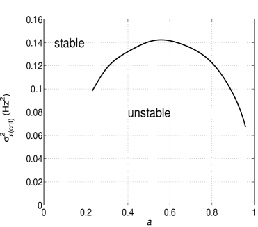
FIG. 4.: The phase diagram for information transmission, for $r=2$ and $\sigma_{J}^{2}=1/C$. (a) Threshold $\xi_{0}=-0.4$. (b) Threshold $\xi_{0}=+0.0$. (c) Threshold $\xi_{0}=+0.4$. (d) Threshold $\xi_{0}=+0.8$.

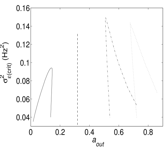
FIG. 5.: The marginal noise variance as a function of the sparseness of the output distribution. The solid line represents the curve for $\xi_{0}=-0.40$ (the same situation as Fig. 4a), the dashed curve $\xi_{0}=0.0$, the dot-dashed curve $\xi_{0}=+0.40$, and the dotted curve $\xi_{0}=+0.80$. Note that for $\xi_{0}=0.0$ the output sparseness is fixed at $1/\pi$, as explained in the text, so this particular line is not informative about the relative region of instability.