Thermodynamics of the 2D Hubbard model

Abstract

A theoretical analysis of the thermodynamic response functions of the 2D single-band Hubbard model is carried out by means of the composite operator method. It is shown that all the features of these quantities can be explained by looking at the dependence of the thermodynamic variables on their conjugate ones, that is, for example, the relation between entropy and temperature, chemical potential and particle concentration, double occupancy and on-site Coulomb repulsion. In this way, the electronic specific heat and the entropy per site are determined in the paramagnetic phase. Also, for the electronic specific heat and internal energy we present three different schemes of calculation. A comprehensive comparison among them for the interacting case opens the possibility to obtain a deep theoretical understanding of the computed quantities whereas, for the non-interacting case, only confirms the internal consistency of the thermodynamic approach. It is found that the numerical data from quantum Monte Carlo techniques for the internal energy and electronic specific heat are well reproduced by determining them through the first and second temperature derivatives of the chemical potential. The anomalous normal state properties in hole-doped cuprate high $T_{c}$ superconductors are also well described. Actually, the results for the linear coefficient of the electronic specific heat are in agreement with those obtained by using a pure fermionic theoretical scheme. Indeed, the results for the Wilson ratio seem to confirm the same scenario. Finally, we obtain several characteristic crossing points for the response functions when plotted versus some thermodynamic variables. These peculiar features indicate the existence of more than one energy scale competing with thermal excitations and indicate, as already noted by Volhardt, a crossover from a non-interacting to a highly correlated behavior.

I INTRODUCTION

It is believed, on both experimental and theoretical grounds, that superconductivity and charge transport in high $T_{c}$ cuprates are mostly confined to the $CuO_{2}$ planes [1,2]; and hence the attention of many physicists has been dedicated to 2D models which contain as an essential feature a competition between the band picture and highly correlated many body effects. Of course, some features of the phase diagram, like the existence of a finite Néel temperature, can only be explained by adding a coupling between the planes.

The bonding combination of $Cu$ and $O$ orbitals turns out to be quite deep below the Fermi level, so that no dynamical freedom is left to treat $d$ and $p$ orbitals separately [3] (there are some strong experimental evidences, mostly based on the study of the Knight shift, that in the $CuO_{2}$ plane one spin degree of freedom is observed [4]). Through the Pauli principle, the energy of the $p$ electron excitation is, for example, largely modified by the change of charge and spin states of the neighboring $Cu$ ions. A $p$ electron and charge and spin fluctuations on neighboring $Cu$ ions are simultaneously excited so that electronic excitations are formed on a $CuO_{2}$ cluster as a whole. Then, the resulting complex can be described by a single-band Hubbard model [5].

In the simplest form, the Hubbard model, first introduced to describe the correlations of electrons in a narrow $d$-band of transition metals, contains a kinetic term which describes the motion of the electrons among the sites of the Bravais lattice and an interaction term between electrons of opposite spin on the same lattice site. By varying the model parameters, it is believed that the Hubbard model is capable of describing many properties of strongly correlated fermion systems. Among different examples, the Hubbard Hamiltonian is applicable to describe the metal-insulator transition in a series of transition metal oxides such as $Sr_{1-x}La_{x}TiO_{3}$ [6,7] and $V_{2}O_{3}$ [8-11]. The applicability of the model to the superconducting copper-oxides is related to the fact that upon doping most of these compounds exhibit a metal-insulator Mott transition; the superconducting state is near the Néel state and there are many experimental results [12-15] which show a close relation between the antiferromagnetic correlations in the $Cu-O$ planes and the occurrence of the superconducting phase. However, it is important to stress that an appropriate description of a bad metal with large energy scale spin fluctuations by means of a purely electrostatic Hamiltonian should preserve the symmetry expressed by the Pauli principle that codifies the correct interplay between charge and magnetic configurations [16-18].

Although considerable attention has been devoted to the Hubbard model and significant progress was achieved in understanding ground state properties, particularly at half-filling, static and dynamical spin correlations, the optical conductivity and other observables, a clear comprehension of the low-lying excitations is still lacking [2]. The difficulty is not to be found only in the absence of any obvious small parameter in the strong coupling regime. More deeply, it is due to the difficulty of handling simultaneously itinerant aspects (spatial correlations) and atomic aspects (pronounced on- site quantum fluctuations) [19].

In recent years we have been developing a method of calculation, denominated Composite Operator Method (COM) [17,18,20-32], that has been revealed to be a powerful tool for the description of local and itinerant excitations in strongly correlated systems. In previous papers, we considered the Hubbard electronic operators for the determination of fundamental excitations. A fully self-consistent calculation of the electronic propagator has been realized by means of a constraint with the physical content of the Pauli principle [17, 23-25]. We calculated local quantities, as the double occupancy and the magnetic moment [17,23], the energy per site [24], the chemical potential [24], the magnetic susceptibility [25, 29], the density of states and the quasi-particle spectra [28, 32]. In all the cases, the results show a good agreement with those obtained by numerical simulation. In particular, the results obtained for the magnetic properties can reproduce the unusual characteristics observed in high $T_{c}$ superconducting materials [25, 29, 33]. Therefore, the agreement strengthens the idea that a microscopic single-band model contains the essential physical features of the new class of materials.

In this paper we investigate the electronic specific heat and the entropy per site of the 2D Hubbard model for a paramagnetic ground state. It will be shown that all the features of these quantities can be understood by looking at the dependence of the chemical potential and double occupancy on their conjugate thermodynamic variables, that is, the particle concentration and the on- site Coulomb repulsion, respectively. A comprehensive comparison among different methods to compute the specific heat will shed a new light on the approximation used. It will emerge that in our theoretical scheme, even if dynamical effects in the self-energy are neglected promoting unstable collective asymptotic modes to the role of well-defined quasi-particle excitations, extended spin modes can be captured by properly combining symmetry requirements and extended operatorial basis. Indeed, the presence of a low temperature peak that appears when the low-lying spin states are excited will appear as an important feature shared with the quantum Monte Carlo data [34]. In addition, an alternative fermionic scenario for the computation of the electronic specific heat together with the results for the Wilson ratio will confirm cuprates as dominated by conventional fermionic excitations. An extensive study of the thermodynamic response functions will reveal the existence of critical lines which separate different energy scales created by the interplay between charge and spin modes. In other words a study of thermodynamics quantities, such as the double occupancy, the entropy, the chemical potential, the specific heat, indicates lines in the $U-T$ plane which separate a highly-correlated behavior, dominated by spin and charge fluctuations and a non-interacting behavior, dominated by thermal fluctuations. In particular, there emerges a region of filling where the entropy reduces by increasing the filling signalling the set up of an ordered phase. For $T\to 0$ there is a well-defined marginal concentration where a quantum phase transition occurs. A detailed comparison with the non-interacting case will be also presented throughout the paper.

The plan of the article is as follows. In the next Section we present the 2D Hubbard model and the electron propagator in the COM. In Sec. III we review experimental data for some thermodynamic properties. The results for the electronic specific heat are presented in Sec IV, where a theoretical understanding of the different ways to compute the specific heat is also presented. Section V is devoted to a discussion of double occupancy. In Sec. VI the results for the chemical potential versus temperature are discussed. The entropy is analyzed in Sec VII. Some concluding remarks are presented at the end.

II ELECTRON PROPAGATOR IN THE HUBBARD MODEL

The Hubbard model is defined by

$$H=\sum_{i,j}t_{ij}c^{\dagger}(i)\cdot c(j)+U\sum_{i}n_{\uparrow}(i)n_{\downarrow}(i)-\mu\sum_{i}n(i)$$ (1)

The notation is the following. The variable $i$ stands for the lattice vector ${\rm\bf R}_{i}$. $\left\{c(i),c^{\dagger}(i)\right\}$ are annihilation and creation operators of $c-$electrons at site $i$, in the spinor notation:

$$c=\left({c_{\uparrow}\atop c_{\downarrow}}\right)\qquad c^{\dagger}=\left(c^{\dagger}_{\uparrow}\quad c^{\dagger}_{\downarrow}\right)$$ (2)

$t_{ij}$ denotes the transfer integral and describes hopping between different sites; the U term is the Hubbard interaction between two $c-$electrons at the same site with

$$n_{\sigma}(i)=c^{\dagger}_{\sigma}(i)c_{\sigma}(i)$$ (3)

being the charge-density operator per spin $\sigma$. $n(i)$ is the total charge-density operator. $\mu$ is the chemical potential. In the nearest neighbor approximation, for a two-dimensional cubic lattice with lattice constant $a$, we write the hopping matrix $t_{ij}$ as

$$t_{ij}=-4t\alpha_{ij}=-4t{1\over N}\sum_{\rm\bf k}e^{i{\rm\bf k}\cdot(\rm\bf r_{i}-{\rm\bf R}_{j})}\alpha({\rm\bf k})$$ (4)

where

$$\alpha({\rm\bf k})={1\over 2}\left[\cos(k_{x}a)+\cos(k_{y}a)\right]$$ (5)

The scale of the energy has been fixed in such a way that $t_{ii}=0$. It should be noted that since the interactions are restricted to the same site, the dimensionality of the system comes in only when a specific form for $\alpha({\rm\bf k})$ is taken. In other words, the stabilization of eventual cooperative phenomena is uniquely governed by the band dispersion.

The point of view adopted in the COM is that the Heisenberg operators $\{c(i),c^{\dagger}(i)\}$ are not good candidates as a basis for calculations. Because of strong correlations the $c-$electrons loose their identity and new fields, whose properties are self-consistently determined by the dynamics and by the symmetries of the model, together with the boundary conditions, might be more appropriate as a starting point for the physical description of the system. Due to the on-site Coulomb interaction, it is known that two sharp features develop in the band structure which correspond to the Hubbard subbands and describe interatomic excitations mainly restricted to subsets of the occupancy number. Indeed, a first natural choice for composite fields is given by the Hubbard constrained electronic operators

$$\xi(i) = [1-n(i)]c(i)$$ (6)

$$\eta(i) = n(i)c(i)$$ (7)

describing the transitions $(n=0)\Longleftrightarrow(n=1)$ and $(n=1)\Longleftrightarrow(n=2)$, respectively. The two-point retarded thermal Green’s function is defined as

$$S(i,j)=\langle R[\Psi(i)\Psi^{\dagger}(j)]\rangle\ ,$$ (8)

where $\Psi(i)$ is the doublet composite operator

$$\Psi(i)={\xi(i)\choose\eta(i)}$$ (9)

The bracket $\langle\ldots\rangle$ indicates the thermal average and $R$ is the usual retarded operator.

In previous papers, we have shown that the determination of the single-particle Green’s function (2.8) can be realized in a fully self-consistent way once a unique approximation is made [17, 23-25]. This approximation consists in neglecting the dynamical part in the self-energy and corresponds to a pole expansion of the spectral intensities. As shown in Ref. 23-25, by considering time translational invariance and no magnetic order, the single-particle electronic propagator has the following expression

$$S_{cc}(i,j) = \langle R[c(i)c^{\dagger}(j)]\rangle=$$ (10)

$$= {i\Omega\over(2\pi)^{3}}\int_{\Omega_{B}}d^{2}kd\omega e^{i{\rm\bf k}\cdot({\rm\bf R}_{i}-{\rm\bf R}_{j})-i\omega(t_{i}-t_{j})}[1-f_{F}(\omega)]\left[{A_{1}({\rm\bf k})\over\omega-E_{1}({\rm\bf k})+i\eta}+{A_{2}({\rm\bf k})\over\omega-E_{2}({\rm\bf k})+i\eta}\right]$$ (11)

$\Omega$ and $\Omega_{B}$ being the volume of the unit cell in the direct and reciprocal space, respectively. $f_{F}(\omega)$ is the Fermi distribution function. $E_{1}({\rm\bf k})$ and $E_{2}({\rm\bf k})$ are the energy spectra

$$E_{1,2}({\rm\bf k})=R({\rm\bf k})\pm Q({\rm\bf k})$$ (12)

$A_{1}({\rm\bf k})$ and $A_{2}({\rm\bf k})$ are the spectral intensities

$$A_{1}({\rm\bf k})= \displaystyle{1\over 2}\left[1-{U(1-n)\over 2Q({\rm\bf k})}+{m_{12}({\rm\bf k})\over 2I_{11}I_{22}Q({\rm\bf k})}\right]$$ (13)

$$A_{2}({\rm\bf k})= \displaystyle{1\over 2}\left[1+{U(1-n)\over 2Q({\rm\bf k})}-{m_{12}({\rm\bf k})\over 2I_{11}I_{22}Q({\rm\bf k})}\right]$$ (15)

with the definitions

$$R = \displaystyle{1\over 2}U-\mu-{2t\over I_{11}I_{22}}\left\{\Delta+\alpha({\rm\bf k})[p+(1-n)I_{22}]\right\}$$ (16)

$$Q = \displaystyle{1\over 2}\sqrt{U^{2}+{1\over I_{11}^{2}I_{22}^{2}}m_{12}^{2}-2U{(1-n)\over I_{11}I_{22}}m_{12}}$$ (18)

$$m_{12}({\rm\bf k}) = 4t\left[\Delta+\alpha({\rm\bf k})\left(p-{n\over 2}\right)\right]$$ (20)

where $n=\langle c^{\dagger}c\rangle$ is the particle density. The parameters $\Delta$ and $p$ are static intersite correlation functions defined as

$$\Delta\equiv\langle\xi^{\alpha}(i)\xi^{\dagger}(i)\rangle-\langle\eta^{\alpha}(i)\eta^{\dagger}(i)\rangle$$ (21)

$$p\equiv{1\over 4}\langle n^{\alpha}_{\mu}(i)n_{\mu}(i)\rangle-\langle[c_{\uparrow}(i)c_{\downarrow}(i)]^{\alpha}c^{\dagger}_{\downarrow}(i)c^{\dagger}_{\uparrow}(i)\rangle$$ (22)

The notation $c^{\alpha}(i)$ stands to indicate the field $c$ on the first neighbor sites:

$$c^{\alpha}(i)=\sum_{j}\alpha_{ij}c(j)$$ (23)

We are also using the following notation

$$I_{11}=1-n/2\qquad I_{22}=n/2$$ (24)

A crucial point in the calculation of the propagator (2.10) is the implementation of the Pauli principle by means of constraining equations to determine the internal parameters $\mu$, $\Delta$ and $p$. Use of this principle leads to the self-consistent equations [23, 25]

$$n=1-G_{0}+U(1-n)F_{0}$$

$$\Delta={1-n\over 2}G_{1}-{U\over 2}F_{1}+{(1-n)\over 2I_{11}I_{22}}B_{1}$$ (25)

$$pF_{1}=I_{22}F_{1}-\Delta F_{0}$$

where

$$F_{n}={\Omega\over 2(2\pi)^{2}}\int_{\Omega_{B}}d^{2}k[\alpha({\rm\bf k})]^{n}f({\rm\bf k})$$

$$G_{n}={\Omega\over 2(2\pi)^{2}}\int_{\Omega_{B}}d^{2}k[\alpha({\rm\bf k})]^{n}g({\rm\bf k})$$ (26)

$$B_{n}={\Omega\over 2(2\pi)^{2}}\int_{\Omega_{B}}d^{2}k[\alpha({\rm\bf k})]^{n}f({\rm\bf k})m_{12}({\rm\bf k})$$

with

$$f({\rm\bf k})=\displaystyle{T_{1}({\rm\bf k})-T_{2}({\rm\bf k})\over 2Q({\rm\bf k})}\qquad g({\rm\bf k})=[T_{1}({\rm\bf k})+T_{2}({\rm\bf k})]$$ (27)

(28)

$$T_{i}({\rm\bf k})=\displaystyle\tanh\left({E_{i}({\rm\bf k})\over 2k_{B}T}\right)$$ (29)

The recovery of the Pauli principle, very often violated by other approximations, assures a dynamics bounded to the Hilbert space capable of describing in a correct way the interplay between the charge and the magnetic configurations. Furthermore, we have shown [35] that in the two-pole approximation [36] the set of self-consistent equations (2.18) is the only one which restores the particle-hole symmetry and the Pauli principle, which are intimately connected.

It is possible to go beyond the two-pole approximation by enlarging the set of asymptotic fields [18, 20-22] or by taking into account the dynamical corrections to the self-energy [31,32].

III THERMODYNAMICS AS REVEALED BY EXPERIMENTS

The electronic specific heat $C(T)$ of cuprate high-$T_{c}$ superconductors has been measured. In particular $C(T)$ of $La_{2-x}Sr_{x}CuO_{4}$ [37, 38] has been studied for $0.03<x<0.45$ in the range of temperatures between 1.5 and 300 K, and of $YBa_{2}Cu_{3}O_{6+y}$ [39] for $0.16\leq y\leq 0.97$ between 1.8 and 300 K. From these experiments the following behavior has been observed for the coefficient $\gamma=C/T$ of the normal state specific heat:

a) for fixed temperature, $\gamma(x,T)$ increases with doping;

a1) in the case of $La_{2-x}Sr_{x}CuO_{4}$, $\gamma(x,T)$ exhibits a rather sharp maximum at $x\approx 0.25$ (near the doping where superconductivity disappears), then starts to decrease; the same behavior for $\gamma(x,T)$ has been estimated in Ref. 40, but with a peak located around $x\approx 0.18$, close to the optimal doping; for $La_{2-x}Ba_{x}CuO_{4}$ [41] a maximum has been observed at $x\approx 0.22$;

a2) in the case of $YBa_{2}Cu_{3}O_{6+y}$, $\gamma(x,T)$ increases smoothly to a plateau or two broad maxima, situated at $y\approx 0.6$ and $y\approx 0.9$, respectively;

b) for fixed doping, $\gamma(x,T)$ as a function of temperature exhibits a broad peak moving to lower temperatures with increasing the dopant concentration;

c) further increasing $y$, the T-dependence weakens and in the region of high doping no increase is observed. For $YBa_{2}Cu_{3}O_{6+y}$, no substantial increase is observed for $y>0.8$.

As noticed by Vollhardt [42], there is a peculiar feature of the specific heat observed in a large variety of systems. The specific heat curves versus T, when plotted for different, not too large, values of some thermodynamic variable, intersect at one or even two well defined temperatures. In ${}^{3}He$ the specific heat $C(T,P)$ curves versus T at different pressures P intersect at a well defined temperature [43,44]; in heavy fermions $CeAl_{3}$ [45] and $UBe_{13}$ [46] upon change of $P$, $UPt_{3-x}Pd_{x}$ [47] and $CePt_{3}Si_{1-x}Ge_{x}$ [48] upon change of $x$, $CeCu_{6-x}Au_{x}$ when either P [49] or the magnetic field B [50] is varied; in semi-metal, $Eu_{0.5}Sr_{0.5}As_{3}$ [51] upon change of B.

The following properties have been observed for the entropy $S$ [38, 39, 52]:

a) for a given temperature, $S$ increases with doping;

a1) in the case of $La_{2-x}Sr_{x}CuO_{4}$ [38], $S(x,T)$ reaches a maximum in the vicinity of $x\approx 0.25$, then decreases;

a2) in the case of $YBa_{2}Cu_{3}O_{6+y}$ [39, 52], $S$ reaches a maximum in the vicinity of $y\approx 0.97$;

b) for a given dopant concentration, $S$ exhibits a superlinear dependence on the temperature;

c) the normal state entropy as a function of $T$ extrapolates to a negative value at $T=0K$;

d) there is a striking numerical correlation between $S/T$ and $a\chi_{0}$, where $\chi_{0}$ is the bulk susceptibility and $a$ is the Wilson ratio.

IV ELECTRONIC SPECIFIC HEAT

A GENERAL FORMULAS

The specific heat $C(T)$ is defined as

$$C(T)={dE\over dT}$$ (30)

where $E$ is the internal energy density, given by the thermal average of the Hamiltonian

$$E={1\over N}\langle H\rangle$$ (31)

$N$ being the number of sites. Calculation of internal energy by means of Eq. (4.2) will generally require the calculation of two-particle Green’s functions. An alternative way to calculate the internal energy is the following. By introducing the Helmholtz free energy per site

$$F=E-TS$$ (32)

where $S$ is the entropy per site, from the thermodynamics we have

$$S=-\left({\partial F\over\partial T}\right)_{n}\qquad\mu=\left({\partial F\over\partial n}\right)_{T}\qquad\left({\partial S\over\partial n}\right)_{T}=-\left({\partial\mu\over\partial T}\right)_{n}$$ (33)

Then, it is straightforward to obtain the following formulas

$$F(T,n)=\int_{0}^{n}\mu(T,n^{\prime})dn^{\prime}$$ (34)

$$S(T,n)=-\int_{0}^{n}\left({\partial\mu\over\partial T}\right)_{n^{\prime}}dn^{\prime}$$ (35)

$$E(T,n)=\int_{0}^{n}\left[\mu(T,n^{\prime})-T\left({\partial\mu\over\partial T}\right)_{n^{\prime}}\right]dn^{\prime}$$ (36)

from which the specific heat turns out to be

$$C(T,n)=-T\int_{0}^{n}\left({\partial^{2}\mu\over\partial T^{2}}\right)_{n^{\prime}}dn^{\prime}$$ (37)

In this scheme the thermodynamic quantities are all expressed through the chemical potential, whose determination requires the knowledge of the single-particle Green’s function.

Summarizing, we have two distinct ways to calculate the internal energy, based on the use of Eqs. (4.2) and (4.7). In principle these equations are equivalent and lead to the same result when an exact solution is available. However, the situation drastically changes when approximations are involved and different results can be obtained. Indeed an open problem in Condensed Matter Physics is to find a unique consistent scheme of approximation capable of treating on an equal footing, both one- and two-particle Green’s functions.

Sometimes in the literature the internal energy for electronic systems is calculated by means of the expression

$$E=\int_{-\infty}^{+\infty}d\omega N(\omega)f_{F}(\omega)\omega$$ (38)

where $N(\omega)$ is the density of states. However, Eq (4.9) is based on the assumption that the system admits a description in terms of fermionic quasi-particles. It is well known that the correlation among the original electrons can generate extended bosonic modes, and use of expression (4.9) requires special attention. By general argument it can be shown that for interacting systems the correct expression for the internal energy, calculated by means of the density of states, is given by

$$E=\int_{-\infty}^{+\infty}d\omega N(\omega)f_{F}(\omega)\omega-\langle H_{I}\rangle$$ (39)

where $\langle H_{I}\rangle$ is the non-quadratic part of the Hamiltonian in the chosen canonical representation.

B NON-INTERACTING CASE

To discuss the specific heat it is useful at first to consider the non-interacting [i.e. U=0] Hubbard model. In this case the thermal retarded Green’s function can be exactly calculated and has the expression

$$S_{cc}(i,j) = \langle R[c(i)c^{\dagger}(j)]\rangle$$ (40)

$$= {i\Omega\over(2\pi)^{3}}\int_{\Omega_{B}}d^{2}kd\omega e^{i{\rm\bf k}\cdot({\rm\bf R}_{i}-{\rm\bf R}_{j})-i\omega(t_{i}-t_{j})}[1-f_{F}(\omega)]{1\over\omega-E({\rm\bf k})+i\eta}$$ (41)

where the energy spectrum has the expression

$$E({\rm\bf k})=-\mu-4t\alpha({\rm\bf k})$$ (42)

The chemical potential is determined as a function of n and T by means of the equation

$$n={2\Omega\over(2\pi)^{2}}\int_{\Omega_{B}}d^{2}kf_{F}[E({\rm\bf k})]=1-{\Omega\over(2\pi)^{2}}\int_{\Omega_{B}}d^{2}kT({\rm\bf k})$$ (43)

where we put

$$T({\rm\bf k})=\tanh\left({E({\rm\bf k})\over 2k_{B}T}\right)$$ (44)

As we discussed above, we have different ways of calculating the free energy. In the non-interacting case, where an exact solution is available, all different procedures must give the same result. Since this point will acquire some relevance in the interacting case, we shall examine this in detail.

In the non-interacting case the density of states is given by

$$N(\omega)={\Omega\over(2\pi)^{2}}\int_{\Omega_{B}}d^{2}k\delta[\omega-E({\rm\bf k})]$$ (45)

By substituting this expression into Eq. (4.10) we have

$$E={4t\Omega\over(2\pi)^{2}}\int_{\Omega_{B}}d^{2}k\alpha({\rm\bf k})T({\rm\bf k})$$ (46)

where a factor 2 has been included in order to take into account the spin degree of freedom.

The same result is obtained by taking the thermal average of the Hamiltonian

$$E=8t\langle c^{\alpha}(i)c^{\dagger}(i)\rangle={4t\Omega\over(2\pi)^{2}}\int_{\Omega_{B}}d^{2}k\alpha({\rm\bf k})T({\rm\bf k})$$ (47)

where use has been made of the expression (4.10) for the single-particle Green’s function.

The proof that use of Eq. (4.7) leads to the same result requires some work. By taking the derivative with respect to T of Eq. (4.12) we have

$${\partial\mu\over\partial T}={1\over T}\left[\mu+4t{V_{1}\over V_{0}}\right]$$ (48)

where

$$V_{n}={\Omega\over(2\pi)^{2}}\int_{\Omega_{B}}d^{2}k{[\alpha({\rm\bf k})]^{n}\over\cosh^{2}(E/2k_{B}T)}$$ (49)

By considering that the derivative with respect to $n$ of Eq. (4.12) gives

$${V_{1}\over V_{0}}={\int_{\Omega_{B}}d^{2}k\alpha({\rm\bf k}){\partial T({\rm\bf k})\over\partial n}\over\int_{\Omega_{B}}d^{2}k{\partial T({\rm\bf k})\over\partial n}}=-{\Omega\over(2\pi)^{2}}{\partial\over\partial n}\int_{\Omega_{B}}d^{2}k\alpha({\rm\bf k})T({\rm\bf k})$$ (50)

substitution of (4.17) into (4.8) leads to

$$E(T,n)={4t\Omega\over(2\pi)^{2}}\int^{n}_{0}{\partial\over\partial n^{\prime}}\left[\int_{\Omega_{B}}d^{2}k\alpha({\rm\bf k})T({\rm\bf k})\right]dn^{\prime}={4t\Omega\over(2\pi)^{2}}\int_{\Omega_{B}}d^{2}k\alpha({\rm\bf k})T({\rm\bf k})$$ (51)

This concludes the proof that in the non-interacting case all expressions (4.2), (4.3) and (4.8) give the same result. We also note that the specific heat can be calculated by means of the following expression

$$C(T,n)=-{8t^{2}\over k_{B}T^{2}}\left[{V^{2}_{1}\over V_{0}}-V_{2}\right]$$ (52)

In Figs. 1 and 2 the linear coefficient of the electronic specific heat $\gamma(T,n)$ is plotted as a function of temperature and filling, respectively.

a For a fixed filling $\gamma(T,n)$ first increases as a function of T, exhibits a maximum at a certain temperature $T_{m}$, and then decreases. The value of $T_{m}$ decreases by increasing the filling. At half-filling $T_{m}$ is zero and $\gamma(T,n)$ diverges as $T\to 0$; this is an effect of the van Hove singularity (vHs). The temperature behavior of $\gamma(T,n)$ is similar to the one exhibited by the static uniform spin magnetic susceptibility $\chi_{0}$ [12,25], whereas the doping dependence is different.

b1. At $T=0$, $\gamma(T,n)$ increases by increasing the filling, diverges at $n=1$ and then decreases.

b2. At finite temperature the peak splits in two peaks, symmetric with respect to $n=1$. The distance between the two peaks increases by increasing T.

FIG. 1.: The linear coefficient of the normal state specific heat $\gamma(T,n)$ of the non-interacting 2D Hubbard model is plotted as a function of the temperature for various values of the particle density.

This is shown in Fig. 2, where $\gamma(T,n)$ is plotted as a function of the filling at various temperatures. The shift of the two peaks with respect to $n=1$ increases by increasing T.

FIG. 2.: $\gamma(T,n)$ of the non-interacting 2D Hubbard model is plotted as a function of the filling for various values of the temperature.

C INTERACTING CASE

In the interacting case the expressions (4.2) and (4.7) for the internal energy give different results. By recalling (2.10), Eq. (4.2) gives

$$E_{H}=E_{F}-UD$$ (53)

where $D$ is the double occupancy. We use $E_{H}$ to indicate that the internal energy has been calculated by the average of the Hamiltonian. $E_{F}$ is the part of the internal energy calculated on the assumption of only fermionic elementary excitations

$$E_{F}\equiv \int_{-\infty}^{+\infty}d\omega N(\omega)f_{F}(\omega)\omega$$ (54)

$$= {\Omega\over(2\pi)^{2}}\int_{\Omega_{B}}d^{2}k\left\{\left[1-T_{1}({\rm\bf k})\right]\left[E_{1}({\rm\bf k})+\mu\right]A_{1}({\rm\bf k})+[1-T_{2}({\rm\bf k})][E_{2}({\rm\bf k})+\mu]A_{2}({\rm\bf k})\right\}$$ (55)

(4.23)

Alternatively, we have seen that the internal energy and the specific heat can be calculated by means of Eqs. (4.8) and (4.9). This procedure requires a knowledge of the first and second temperature derivatives of the chemical potential. Let us define

$$\mu_{n}={\partial^{n}\mu\over\partial T^{n}}\qquad\Delta_{n}={\partial^{n}\Delta\over\partial T^{n}}\qquad p_{n}={\partial^{n}p\over\partial T^{n}}$$ (56)

By taking the first derivative with respect to T of the self-consistent equations (2.18), we obtain

$$G^{(1)}_{0}=U(1-n)F^{(1)}_{0}$$

$$\Delta_{1}={1-n\over 2}G^{(1)}_{1}-{U\over 2}F_{1}^{(1)}+{(1-n)\over 2I_{11}I_{22}}B_{1}^{(1)}$$ (57)

$$p_{1}F_{1}+pF^{(1)}_{1}=I_{22}F^{(1)}_{1}-\Delta_{1}F_{0}-\Delta F^{(1)}_{0}$$

where

$$F^{(m)}_{n}={\partial^{m}F_{n}\over\partial T^{m}}\qquad G^{(m)}_{n}={\partial^{m}G_{n}\over\partial T^{m}}\qquad B^{(m)}_{n}={\partial^{m}B_{n}\over\partial T^{m}}$$ (58)

Explicit calculation of the derivatives defined in Eq. (4.26) shows that the equations (4.25) provide a set of linear algebraic equations for the three parameters $\mu_{1}$, $\Delta_{1}$, $p_{1}$, as functions of the parameters $\mu$, $\Delta$, $p$. In the same way, by taking the second derivative with respect to T of Eqs. (2.18) we obtain

$$G^{(2)}_{0}=U(1-n)F^{(2)}_{0}$$

$$\Delta_{2}={1-n\over 2}G^{(2)}_{1}-{U\over 2}F_{1}^{(2)}+{(1-n)\over 2I_{11}I_{22}}B_{1}^{(2)}$$ (59)

$$p_{2}F_{1}+2p_{1}F^{(1)}_{1}+pF^{(2)}_{1}=I_{22}F^{(2)}_{1}-\Delta_{2}F_{0}-2\Delta_{1}F^{(1)}_{0}-\Delta F^{(2)}_{0}$$

These equations provide a set of linear algebraic equations for the three parameters $\mu_{2}$, $\Delta_{2}$, $p_{2}$ as functions of the parameters $\mu$, $\Delta$, $p$, $\mu_{1}$, $\Delta_{1}$, $p_{1}$. Once the self-consistent calculation of the three parameters $\mu$, $\Delta$, $p$ has been performed by means of the set (2.18), then the calculation of the first and second derivatives of the chemical potential reduces to the solution of simple linear equations.

In the interacting case, because of the approximation used, the different procedures to calculate the internal energy give different results. At first we shall compare our theoretical results with the data obtained by numerical analysis. The specific heat $C(T)$ of the 2D Hubbard model has been recently calculated in Ref. 34 by using quantum Monte Carlo techniques. In particular, the Monte Carlo data for the energy per site $E=\langle H\rangle/N$ have been fitted by polynomials and the specific heat has been calculated by taking derivatives from these polynomials analytically. Different polynomials have been chosen in different regions of temperature. In the calculation of $E$ , it has been found that finite size effects are strong at weak coupling but become negligible for $U\geq 8$.

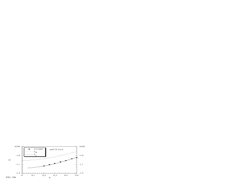
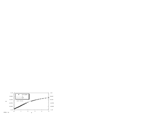
FIG. 3.: The internal energy is plotted as a function of temperature for $U=4$ and $n=0.50$ (a), $n=0.75$ (b), $n=1.0$ (c). The squares are the QMC data of Ref. 34 for $6\times 6$ (a,b) and $8\times 8$ (c) clusters. The dotted and solid lines refer to the theoretical results of the COM for $E_{H}$, $E_{T}$, respectively.

In Fig. 3 we present the internal energy versus temperature in the range $0\leq T\leq 5$ for several values of doping and $U=4$. The results are compared with QMC data of Ref. 34. We are using $E_{T}$ to indicate the solution that comes from Eq. (4.8). As a general feature we observe that $E_{T}$ corresponds to the lowest energy solution and agrees very well with the QMC data, in the entire region of temperature and for all studied dopant concentrations. When U increases, the theoretical solution deviates from QMC in the region of low temperatures, indicating that the antiferromagnetic (AF) correlations are not properly taken into account in the strong coupling regime. This is clearly seen in Fig. 4 where the internal energy is plotted versus U for half-filling.

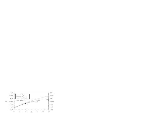
FIG. 4.: The internal energy is plotted as a function of $U$ for $n=1$, $T=0.1$ (a) and $n=0.75$, $T=0.25$ (b). The squares are the QMC data of Ref. 34 for a $8\times 8$ cluster. The dotted and solid lines refer to the theoretical results of the COM for $E_{H}$, $E_{T}$, respectively.

We now consider the specific heat. There are two important features in the Monte Carlo calculations: 1) a low temperature peak that appears when the low-lying spin states are excited, and 2) a high temperature peak which appears when states in the upper Hubbard band are excited. In the weak coupling regime the low temperature peak moves to slightly higher temperature as U increases, reaching a turning point at $U=7$ where the peak is at $T=0.3$. For $U>7$ the peak slowly moves to lower temperatures, as $U$ grows. This indicates the beginning of the strong coupling regime. The broad high temperature peak moves to higher temperatures as $U$ increases, as expected since its presence corresponds to the excitation of states across the gap that grows with $U$. In the strong regime [$U>7$] the position of the charge peak increases linearly with U: $T_{\rm charge}\approx 0.24U$. In addition, all the curves C versus T for several values of U intersect at $T\approx 1.6$. The QMC results for the specific heat of the 2D Hubbard model qualitatively agree with the half-filled 1D Hubbard model [53, 54].

The specific heat $C_{T}=dE_{T}/dT$, calculated by means of Eq. (4.9), is compared with QMC data in Fig. 5 for $U=4$ and various dopant concentrations. At low density the agreement is generally good, in both the weak and strong coupling cases [U=8]. At higher densities the QMC data show a double peak structure, which is enhanced at half filling, but also present at $n=0.75$ for $U=8$.

FIG. 5.: The specific heat is plotted against temperature for $U=4$ and $n=0.5$ (a), $n=0.75$ (b), $n=1.0$ (c). The dotted line represents the QMC data of Ref. 34; the solid line is the result of the COM for $C_{T}$.

In the discussed range of values of $U$ our results do not show a double peak structure. The presence of two peaks in the specific heat has been attributed to the spin and charge excitations. When U is weak the two peaks overlap and there is no resolution. By increasing U the position of the charge peak moves to higher temperatures and we expect to be able to distinguish the two contributions. A study of the specific heat in the strong coupling regime is given in Figs. 6 and 7, where the two expressions $C_{H}=dE_{H}/dT$ and $C_{T}=dE_{T}/dT$ are plotted, respectively, as functions of T at half-filling.

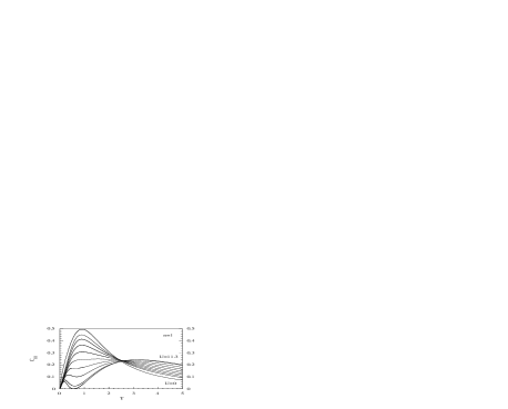
FIG. 6.: The specific heat $C_{H}=dE_{H}/dT$ is plotted against temperature for half-filling and U varying in the range $0\leq U\leq 11.3$

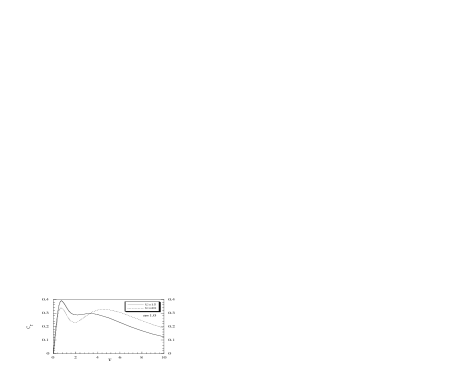
FIG. 7.: The specific heat $C_{T}=dE_{T}/dT$ is plotted against temperature for half-filling and $U=15,20$.

A peak appears at low temperatures when U is rather large [say $U\geq 8$ for $C_{H}$ and $U\geq 15$ for $C_{T}$]. This behavior qualitatively reproduces the QMC results. In order to isolate the spin excitations for lower values of U we can subtract from $C_{T}$ the contribution coming from the pure fermionic part, $C_{F}=dE_{F}/dT$, responsible in large extent for the charge peak structure. This is done in Fig. 8 where we report $C_{T}-C_{F}$ as a function of T for various values of $n$ and $U$. A low-energy excitation appears and its contribution generally increases by increasing $n$ and $U$.

FIG. 8.: The contribution of the low-lying energy excitations to the specific heat, calculated by $C_{T}-C_{F}$, is given versus T for $U=4,8,12$ and $n=1$.

In Ref. 34 the position of the charge peak $T_{\rm charge}$ has been calculated for different values of U. In our analysis when U is large $T_{\rm charge}$ can be calculated from $C_{T}$ and the results lie on the line $T_{\rm charge}=0.24U$. When U is lower, it is not possible to resolve the two peaks. Since the charge excitation mainly comes from the interband fermionic excitations, we can estimate $T_{\rm charge}$ from the calculation of $C_{F}$. This study is shown in Fig. 9, where $T_{\rm charge}$ is plotted versus U. The solid line is the position of the charge peak, calculated by means of $C_{F}$; the triangles denote $T_{\rm charge}$ calculated by means of $C_{T}$; the squares are the QMC results.

FIG. 9.: The position of the charge peak $T_{\rm charge}$ is plotted against U for half-filling. The squares are the QMC data of Ref. 34 for a $8\times 8$ cluster. The solid line and the triangles indicate $T_{\rm charge}$ calculated by means of $C_{F}$ and $C_{T}$, respectively.

The linear coefficient of the specific heat as a function of the particle density has been studied by QMC for $U=8$ and T varying from 0.5 to 3. Unfortunately, due to the sign problem it is not easy to study low temperatures in QMC. A study of $\gamma(x,T)$, by means of $C_{T}$, shows a good agreement for high temperatures, but not at lower temperatures, where QMC results exhibit a strong downward deviation in the region of filling where we should expect an increase of $\gamma(x,T)$ due to the effect of the van Hove singularity.

Up to this point we have performed a detailed and ample comparison with QMC, generally finding a quite reasonable agreement in a large region of values for the model parameters. For intermediate values of U [U=4] the agreement is quite satisfactory. On this basis we are confident that the approximation used is adequate for the 2D Hubbard model and we can pass to examine the next question as to which extent the physics of real systems is retained in the model.

One feature present in a large variety of systems is a characteristic crossing point in the specific heat curves versus T [42-51]. This behavior has been also found in 1D models [53-55] and in the Hubbard model in infinite dimension [19], where a crossing temperature $T=0.59$ has been observed in the range $0.5\leq U\leq 2.5$. For the 2D Hubbard model the same behavior, as predicted by Vollhardt [42] has been observed by means of quantum Monte Carlo calculations [34], where for the case of half-filling a crossing temperature $T=1.6\pm 0.2$ has been observed in the range $2\leq U\leq 12$. In Fig. 10 the specific heat $C_{T}$ is given versus T for half-filling and various values of U. When $n=1$ the curves cross at the same temperature $T\approx 2.0$; when doping is considered the region of crossing spreads out and moves to higher temperatures. From the thermodynamic relations, this crossing temperature $T_{U}$ corresponds to a turning point of the double occupancy as a function of $T$, that is $(\partial^{2}D/\partial T^{2})_{T_{U}}=0$. A study of the function $(\partial^{2}D/\partial T^{2})$ will be done in the next Section.

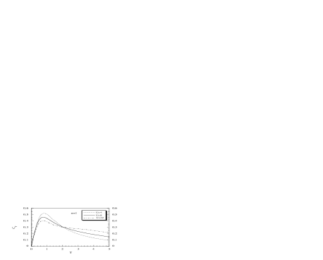
FIG. 10.: The specific heat $C_{T}=dE_{T}/dT$ is plotted against temperature for different values of U and $n=1$.

As mentioned in Section III, the linear coefficient of the specific heat of cuprates exhibits an anomalous behavior in the normal state. To investigate this, in Fig. 11 we present the linear coefficient $\gamma(x,T)$ as a function of the doping $x=1-n$ for various temperatures. As a general behavior we see that by increasing the doping $\gamma(x,T)$ increases up to a certain doping and then decreases. The nature of the peak is due to the fact that the Fermi energy crosses the vHs for a certain critical value $x_{c}$. The value of $x_{c}$ depends on the ratio U/t and varies between 0 and 1/3, as U increases from zero to infinite. For $U/t=4$ it is found $x_{c}=0.27$, very close to the experimental value observed in $La_{2-x}Sr_{x}CuO_{4}$ [37, 38]. At half-filling the Fermi energy ($\epsilon_{F}$) is at the center of the two Hubbard bands; by varying the dopant concentration some weight is transferred from the upper to the lower band, $\epsilon_{F}$ moves to lower energies and crosses the vHs for a critical value of the doping; increasing $x$, further moves $\epsilon_{F}$ away from the vHs. A study of the Fermi surface shows that for $x>x_{c}$ we have a closed surface which becomes nested at $x=x_{c}$ and opens for $x<x_{c}$. An enlarged Fermi surface with a volume larger than the non-interacting one has been reported by QMC calculations [56, 57] and by other theoretical works [58, 59].

FIG. 11.: The linear coefficient of the specific heat $\gamma(x,T)$, calculated from $C_{T}$, is given as a function of the doping $x=1-n$ for $U=4$ and different temperatures.

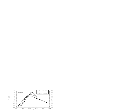
FIG. 12.: The linear coefficient of the specific heat $\gamma(x,T)$ for $La_{2-x}Sr_{x}CuO_{4}$ is shown as a function of the $Sr$ content. The dots are the experimental data for different temperatures, taken from Refs. 37 and 38.

The peak position of $\gamma(x,T)$ depends on the temperature. In the limit of zero temperature a sharp peak is exactly located at $x=x_{c}$. By increasing the temperature the peak moves away from $x_{c}$ and broadens into two peaks. The situation is similar to what we have calculated for the non-interacting case [cfr. Fig. 2]; we find that the role played by the interaction manifests itself through the shift of the vHs and the band structure which creates an asymmetry between the two peaks. The behavior described in Fig. 11 well reproduces the experimental situation.

In the case of $La_{2-x}Sr_{x}CuO_{4}$ the experimental data [37, 38] for $\gamma(x,T)$ are reported in Fig. 12. The peak exhibited by $\gamma(x,T)$ decreases in intensity and moves to lower values of doping when T increases. In the case of $YBa_{2}Cu_{3}O_{6+y}$, the experimental results reported in Ref. 39 are for the higher temperature $T=280K$; $\gamma(x,T)$ increases with doping and presents two broad maxima in the region of high doping.

Interpretation of the experimental results obtained in Ref. 39 for $YBa_{2}Cu_{3}O_{6+y}$ in terms of a sharp feature in the density of states, consistent with ARPES experiments [60], was presented in Refs. 61 and 62. The consistency of thermodynamic data with the presence of a vHs near the Fermi level was shown in Ref. 58 by considering a p-d like-model in the framework of slave-boson mean-field theory in the limit of large U.

We also mention that the specific heat of $La_{2-x}Sr_{x}CuO_{4}$ has been estimated in Ref. 40 from the data for the heat capacity anomaly at the superconducting transition temperature by assuming a BCS-type relation. Under this assumption the authors find the same behavior for $\gamma(x,T)$, but with a peak located around $x\approx 0.18$, close to the optimal doping.

FIG. 13.: The linear coefficient of the specific heat $\gamma(x,T)$, calculated from $C_{T}$, is given as a function of temperature for U=4. In Figs. 19a and 19b the curves have been traced for $x>x_{c}$ and $x<x_{c}$, respectively.

In Figs. 13a and 13b we present the linear coefficient $\gamma(x,T)$ as a function of the temperature for values of the filling $x>x_{c}$ and $x<x_{c}$, respectively. At $x=x_{c}$ we see that $\gamma(x,T)$ diverges as $T\to 0$; this is an effect of the vHs. When $x\neq x_{c}$ the Fermi energy moves away from the vHs and the peak exhibited by $\gamma(x,T)$ moves away from T=0. As shown in Figs. 13a and 13b, $\gamma(x,T)$ as a function of temperature has different behaviors in the two regions $x>x_{c}$ and $x<x_{c}$. In the overdoped region $\gamma(x,T)$ firstly increases as a function of T, exhibits a maximum at a certain temperature $T_{m}$ and then decreases. This behavior is similar to the one exhibited by $\chi_{0}(T)$ [12,25]. As shown in Fig. 13a, when the doping decreases the value of $T_{m}$ moves to lower temperatures. This behavior qualitatively agrees with the non interacting case showing that for $x>x_{c}$ the AF correlations are weak. A different situation is observed in the underdoped region, where $\gamma(x,T)$ is always a decreasing function of T. When we look at the experimental results for $La_{2-x}Sr_{x}CuO_{4}$ [37, 38] and for $YBa_{2}Cu_{3}O_{6+y}$ [39, 52] we find that the behavior of $\gamma(x,T)$ as a function of T in the underdoped region is more similar to that for the non-interacting case, showing that cuprate materials could be conveniently described in terms of a Fermi liquid picture, dominated by the Van Hove singularity. Then, if we want to use the Hubbard model to describe high-$T_{c}$ cuprates, we might assume a scheme for non-interacting -like particles and use Eq. (4.23) to calculate the specific heat. When we do this, we find the results reported in Figs. 14, 15a and 15b.

FIG. 14.: The linear coefficient of the specific heat $\gamma(x,T)$, calculated from $C_{F}$, is given as a function of the doping $x=1-n$ for $U=4$ and different temperatures.

FIG. 15.: The linear coefficient of the specific heat $\gamma(x,T)$, calculated from $C_{F}$, is given as a function of temperature for U=4. In Figs. 15a and 15b the curves have been traced for $x>x_{c}$ and $x<x_{c}$, respectively.

As a function of the doping $\gamma(x,T)$ has a similar behavior for that part dominated by the Van Hove singularity, but the band structure plays a different role. By comparing Figs. 11 and 14 it is worthwhile to stress that the presence of a maximum in $\gamma(x,T)$ does not necessarily indicate a pure fermionic excitation spectrum; it is a consequence of the enhancement in the density of states when the Fermi energy crosses the vHs. This becomes more evident in Fig. 15a and 15b where the temperature dependence is studied at fixed doping. Both in the underdoped and overdoped regions $\gamma(x,T)$ exhibits a maximum at a certain temperature. The behavior given in these figures qualitatively reproduces the experimental situation reported in Ref. 37, 38, 39, 52. The fact that for $YBa_{2}Cu_{3}O_{6+y}$ $\gamma(x,T)$ is always a decreasing function of T when $y>0.8$ is understood because by approaching the critical doping, $T_{m}$ is shifted to low temperatures, below the critical superconducting temperature.

V THE DOUBLE OCCUPANCY

As a simple thermodynamic quantity indicating the degree of correlation of the system, in this Section we study the double occupancy D, defined as the fraction of doubly occupied sites

$$D=\langle n_{\uparrow}n_{\downarrow}\rangle$$ (60)

This quantity can be calculated by means of the expression

$$D={n\over 4}\left[1-G_{0}-UF_{0}\right]$$ (61)

Then, the first and second temperature derivatives of D can be analytically calculated as

$${dD\over dT}=-{n\over 4}\left[G^{(1)}_{0}-UF^{(1)}_{0}\right]\qquad{d^{2}D\over dT^{2}}=-{n\over 4}\left[G^{(2)}_{0}-UF^{(2)}_{0}\right]$$ (62)

once the self-consistent equations have been solved.

We display in Figs. 16a and 16b the temperature dependence of D for various values of U at particle concentrations $n=0.7$ and $n=0.8$. In Fig. 16a the data display a characteristic low temperature behavior: D initially decreases with temperature, reaches a minimum, and increases again. In other words, the curve indicates the presence of a T region where the formation of local magnetic moments is enhanced with increasing T [the double occupancy D determines the local spin-spin correlation function $S^{2}$ through the equation $S^{2}=3(n-2D)/4$]. This behavior is characteristic of incipient localization effects in a strongly correlated Fermi liquid in a regime dominated by spin fluctuations. Starting from the low temperature Fermi liquid regime, when the temperature increases, the system can gain free energy by localizing the particles (i.e. decreasing D) in order to take advantage of a larger spin entropy [19,53]. In the absence of spin excitations one would observe decreasing values with increasing T.

FIG. 16.: The double occupancy $D$ is plotted as a function of the temperature for $n=0.7$, $U=2$ (a) and for $n=0.8$, $U=4$ (b). The arrow in Fig. 22b indicates the temperature $T_{U}$ where the curve changes curvature.

In Fig. 16b D is a monotonic increasing function of temperature. In this case the values of n and U are large enough to inhibit localization effects due to the increase of temperature. To study this behavior in more detail this behavior, the derivative with respect to the temperature of the double occupancy has been analyzed. The results show that for a given T there exists a critical value of U, say $U_{D}(T)$, such that

$${\partial D\over\partial T}<0\qquad{\rm for}\qquad U<U_{D}(T)$$ (63)

$${\partial D\over\partial T}>0\qquad{\rm for}\qquad U>U_{D}(T)$$ (64)

The function $U_{D}(T)$, defined by $\partial D/\partial T=0$, is given in Fig. 17. We note that at T=0 $U_{D}(0)$ coincides with $U_{c}(n,0)$, defined as the critical strength of the on-site Coulomb interaction for which the Fermi energy crosses the vHs at fixed dopant concentration. $U_{D}(T)$ goes to zero for some temperature $T_{D}$. For $n=0.7$ we find that $T_{D}=0.581$. When $T>T_{D}$ we have $\partial D/\partial T>0$ for all values of U. The behavior of $T_{D}$ as a function of $n$ is reported in the Fig. 18. The fact that $(\partial D/\partial T)_{U=U_{D}(T)}=0$ implies that at $U=U_{D}(T)$ the double occupancy does not depend on T. However, the curves of D as function of U for different values of T will not cross in a single point because $U_{D}(T)$ changes with the temperature in a significant way.

FIG. 17.: $U_{D}(T)$ as a function of the temperature for various values of the filling.

At very high temperature $T\gg U$, larger than $T_{U}$ where there is a change in the concavity, D asymptotically tends to the atomic value $n^{2}/4$, as expected. We have seen in the previous section that the specific heat curves versus T for different values of U cross almost at the same point $T_{U}$, determined by the equation

$$\left({\partial^{2}D\over\partial T^{2}}\right)_{T_{U}}=0$$ (65)

FIG. 18.: $T_{D}$ as a function of the filling.

A study of this equation by means of formula (5.3) gives the results plotted in Fig. 19, where $T_{U}$ is plotted versus U for $n=0.75$.

FIG. 19.: $T_{U}$ as a function of the potential intensity U for $n=0.75$.

VI CHEMICAL POTENTIAL VERSUS TEMPERATURE

From the solution of the fermionic propagator and by means of Eqs. (4.25) we obtain the following behavior for the temperature derivative of the chemical potential

$${\partial\mu\over\partial T} < 0\qquad{\rm for}\qquad n<n_{\mu}(T)$$ (66)

$${\partial\mu\over\partial T} = 0\qquad{\rm for}\qquad n=n_{\mu}(T)$$ (67)

$${\partial\mu\over\partial T} > 0\qquad{\rm for}\qquad n>n_{\mu}(T)$$ (68)

FIG. 20.: $n_{\mu}(T)$ as a function of the temperature for different values of U.

The function $n_{\mu}(T)$ is presented in Fig. 20. It can be shown that at $T=0$ $n_{\mu}$ coincides with $n_{c}$, the critical value where the Fermi level crosses the van Hove singularity. But, the temperature dependence of $n_{\mu}(T)$ is remarkably different from the one of $n_{c}(T)$.

FIG. 21.: The chemical potential $\mu$ as a function of the filling for $U=4$ and different temperatures.

Thus, only for $T\to 0$ we may relate the transition $\partial\mu/\partial T<0\Longrightarrow\partial\mu\partial T>0$ to the reversal of the sign of the derivative for the density of states at the Fermi level. Furthermore, we observe that $n_{\mu}(T)$ reaches the value of 1 for some temperature $T_{\mu}$ (for $U=4$ we find $T_{\mu}=0.843$). When $T>T_{\mu}$ we have $\partial\mu/\partial T<0$ for all values of $n$ . The fact that $(\partial\mu/\partial T)_{n=n_{\mu}}(T)=0$ implies that at $n=n_{\mu}(T)$ the chemical potential does not depend on T. Therefore, the curves of $\mu$ as function of $n$ for various values of $T$, reported in Fig. 29, will not cross exactly in the same point as claimed in Ref. 63.

VII THE ENTROPY

The entropy $S(T,n)$, connected to the total number of spin and charge excitations at temperature T and filling $n$, is a bulk thermodynamic quantity uniquely determined by the spectrum of excitations, whose magnitude and temperature dependence provide an important test for proposed theories. Theoretical works available so far are the following. Bipolaron models propose preformed boson charge carriers at $T_{c}$ and behaving classically at higher temperatures. Apart from some inconsistency related to the magnitude of the entropy, these theories have to resort to the existence of thermally excited triplet bipolarons in explaining the deviation of S from a linear T-dependence in underdoped samples [64]. Theoretical studies of the entropy in the strongly correlated electron systems have also been performed in the framework of the statistical spin liquid [65-68]. This scheme is based on the assumption that in the strongly correlated metals the doubly occupied single-spin configurations must be excluded not only in the real space representation, but also in the reciprocal space. By means of the spin liquid statistics, the entropy of localized moments is reproduced when the Mott insulator limit is reached for half-filling. Nevertheless, this over imposed statistics freezes the system in a wrong Hilbert space whenever different choices of the parameters modify the interplay between thermal excitations and electronic interactions. Some theories [3] predict decoupled holon (boson) and spinon (fermion) excitations. In these approaches it is difficult to reconcile the experimentally observed magnitude for the entropy with its partition between statistically independent excitations. Moreover, the striking numerical correlation between $S/T$ and $a\chi_{0}$ is expected for weakly interacting fermions but not if the dominant excitations are those of spinless bosons. In Ref. 63 exact diagonalization studies of the $t-J$ model have been performed; for several thermodynamic quantities a critical doping concentration that marks a change of the Fermi surface character is found.

By means of the relation (4.7), we have calculated the entropy per site $S(T,n)$. Recalling the behavior of $\partial\mu/\partial T$, we see that the entropy must have the following behavior

(i) for $T<T_{\mu}$, $S(T,n)$ increases with increasing particle concentration, reaches a maximum for $n=n_{\mu}$, then decreases (see Fig. 22a);

(ii) for $T>T_{\mu}$, $S(T,n)$ always increases with increasing particle concentration (for $U=4$ we find $T_{\mu}=0.843$) as is shown in Fig. 22b.

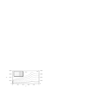
FIG. 22.: The entropy is plotted versus the particle density for $U=4$ and different temperatures.

Again the peak structure reflects a Fermi level crossing the vHs at the critical doping. This behavior is in agreement with the experimental data from Refs. 38, 39 and 52. Indeed, the experiments show a well defined peak structure in a large region of temperature (from 40K to 320K); furthermore, the position of the peak slightly changes with temperature. In the theoretical analysis the position of the peak as a function of temperature is governed by $n_{\mu}(T)$, reported in Fig. 20, that shows a smooth variation in the region of physical relevance ($T<0.05$). In Fig. 23 the entropy versus the particle concentration is reported for various values of the Coulomb interaction.

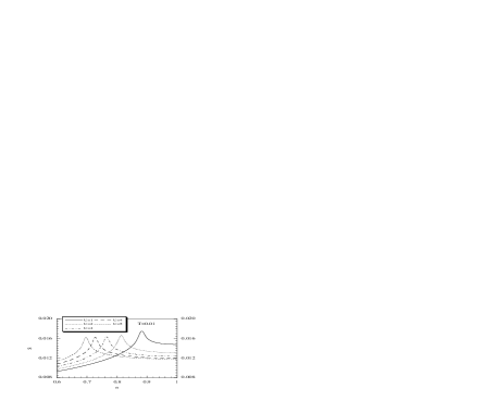
FIG. 23.: The entropy is plotted versus the particle density for $T=0.01$ and different values of U.

The maximum of the entropy shifts to lower values of $n$ by increasing U, varying between 1 and 2/3 when U varies from zero to $\infty$. In Fig. 24, we see that for $T=0.4$ all entropy curves for different U cross at the same particle concentration. By comparison with figure 21 and by numerical analysis, we see that the crossing point is exactly the critical concentration $n_{\mu}(T)$. Recalling the Maxwell relation

$$\left({\partial S\over\partial U}\right)_{T}=-\left({\partial D\over\partial T}\right)_{U}$$ (69)

the behavior shown in Fig. 22 implies $(\partial D/\partial T)_{n=n_{\mu}}=0$. If we remember that the double occupancy $D$ determines the local spin-spin correlation function, it is clear that a sign reversal of its derivative with respect to the temperature represents a crossover from a regime dominated by spin fluctuations, where S is a decreasing function of U, to another regime favouring charge fluctuations (electronic delocalization), where the entropy is an increasing function of U.

FIG. 24.: The entropy is reported versus the particle density for $T=0.4$ and different values of U.

In Figs. 25 and 26 we report the temperature dependence of $S$ and $S/T$ for several dopant concentrations. The curves have a qualitative agreement with the experimental ones [38,39,52]. In Fig. 25a, where $x>x_{c}$, S is a decreasing function of $x$ at a fixed temperature; the opposite behavior is observed in Fig. 25b.

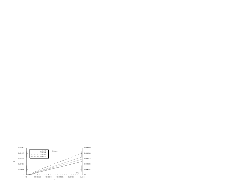
FIG. 25.: The entropy is plotted versus the temperature for $U=4$. The range of filling is $x>x_{c}$ for (a) and $x<x_{c}$ for (b)

In the limit of zero temperature the entropy goes to zero by a linear law. When T increases the entropy deviates from the linear behavior. In the region $0.01\leq T\leq 0.1$ the temperature dependence is well described by the law

$$S(T)=S_{0}+S_{1}T+S_{2}T^{2}$$ (70)

where the coefficients $S_{0}$, $S_{1}$, $S_{2}$ are strongly dependent on the filling.

FIG. 26.: $S/T$ is plotted versus the temperature for $U=4$. The range of filling is $x>x_{c}$ for (a) and $x<x_{c}$ for (b)

It is worth noticing that in the limit of large temperatures (a weak point of the statistical spin liquid [65-68]) our results for the entropy asymptotically agree with the exact expression

$$\lim_{T\to\infty}S(T,n)=2\ln 2-n\ln n-(2-n)\ln(2-n)$$ (71)

For non-interacting fermions at $T=0K$ we have

$$\gamma=a\chi_{0}$$ (72)

where $\chi_{0}$ is the bulk susceptibility and $a$ is the Wilson ratio

$$a={\pi^{2}\over 3}$$ (73)

In the case of $La_{2-x}Sr_{x}CuO_{4}$ [38] and of $YBa_{2}Cu_{3}O_{6+y}$ [39,52,69], there is a striking numerical correlation between $S/T$ and $a\chi_{0}$. As noticed by Loram et al., this resemblance shows that the total spin+charge spectrum over all moments ${\rm\bf k}$ (from S) and the ${\rm\bf k}=0$ spin spectrum (from $\chi_{0}$) have a similar energy dependence. Also, experimental evidences suggest that the low-energy excitations are predominantly those of conventional fermions, and that the substantial T dependencies of $S/T$ and $\chi_{0}$ are primarily determined by the energy dependence of the single-particle density of states in the vicinity of the Fermi level.

FIG. 27.: $S/T\chi_{0}$ is plotted versus the temperature for $U=4$ and different fillings.

In Fig. 27 we present $S/T\chi_{0}$ as a function of the temperature for various values of doping (i.e., $0.03\leq x\leq 0.27$). For all values of dopant concentration $S/T\chi_{0}$ is almost constant over a wide range of temperatures.

In addition, the value of $S/T\chi_{0}$ is less than the non-interacting one. This is due to the fact that by introducing interaction the number of microscopic states accessible to the same macroscopic state is reduced (i.e., the entropy per site) whereas the susceptibility is increased by incipient localization effects.

In order to obtain a better understanding of how the thermodynamics of an electronic liquid is modified by the interaction, we have performed a study of non-interacting Hubbard model (i.e. $U=0$). What we learn from the study of this model is that the critical value (i.e. half-filling) above which the entropy looks a decreasing function of the filling is uniquely fixed by the statistics. The temperature has no role. On the contrary, in the interacting case the energy scale of charge configurations has a crucial role in the region of particle concentration between $n_{\mu}$ and half-filling. For $n_{\mu}<n<1$ there is a critical temperature $T_{\mu}$, depending on the filling, above which the behavior is similar to the non-interacting case [i.e. where $\partial S/\partial n$ becomes positive, or where $\partial\mu/\partial T$ becomes negative].

We now consider the physical origin of these results. In the non-interacting case the combinatorics dictated by the Fermi statistics governs the behavior of the entropy. This can be understood if we think that for the single-site problem the entropy has the values 0, $\ln 2$ and 0 for occupancy 0, 1 and 2, respectively. In the interacting case it is natural to look for a critical value of the filling above which the number of permutations satisfying the restrictions of the boundary conditions starts to decrease. For $n_{\mu}<n<1$, because of the Coulomb interaction, by increasing the particle density the number of microscopic realizations, accessible to the same observable macroscopic state, decreases [the Pauli principle is obviously crucial for a correct counting]. This is true only if the thermal excitations do not exceed the energy scale fixed by the interaction. Definitely, for $0<n<n_{\mu}$ we have a sort of disordered non-interacting state with $\partial S/\partial n>0$, whereas for $n_{\mu}<n<1$ the low-lying excitations characterize a far from random spatial pattern [i.e. $\partial S/\partial n<0$]. In the range $n_{\mu}<n<1$ incommensurate magnetism and superconductivity are experimentally observed [12, 70].

VIII CONCLUDING REMARKS

The 2D single-band Hubbard model has been studied by means of the composite operator method. By considering the Hubbard operators as basic set of fields, which describe interatomic excitations restricted to subsets of the occupancy number, the single-particle electronic propagator has been computed in a fully self-consistent way by means of a quasi-particle scheme capable of coherently integrating dynamics, boundary conditions and symmetry principles.

The paper was devoted to the study of the electronic specific heat and entropy per site in the paramagnetic phase. We analyzed these quantities by looking at the dependence of the thermodynamic variables on their conjugate ones, that is, for example, the relation between entropy and temperature, chemical potential and particle concentration, double occupancy and on-site Coulomb repulsion. Once the self-consistent equations for the single-particle propagator have been solved, we have determined the temperature derivatives of the internal parameters by means of exact linear systems of algebraic equations. The determination of the first and second temperature derivatives of the chemical potential has been revealed crucial in determining the thermodynamic response functions under investigation. For the electronic specific heat and internal energy we have presented three different schemes of calculation. All of them allowed the possibility to obtain a deep theoretical understanding of how and to which extent collective excitations can be retained in the description of thermal response functions. We have obtained a good agreement with the data by quantum Monte Carlo techniques for the electronic specific heat and the internal energy [34]. Further on, although Monte Carlo data shared common features with the results from the calculations through the T-derivative of the chemical potential, the experimental data for cuprates, as revealed by the Wilson ratio and linear coefficient of the electronic specific heat, have shown that in such systems the dominant excitations are those of conventional non-interacting fermions [38].

We obtained several characteristic crossing points for the response functions when reported as functions of some thermodynamic variables. These peculiar features, already evidenced by Vollhardt [42], marked turning points where different response functions evolve from a non-interacting behaviour

(i) the entropy is an increasing function of U;

(ii) the entropy is an increasing function of $n$;

(iii) the double occupancy is a decreasing function of T;

(iv) the T-derivative of the chemical potential is a decreasing function of $n$;

(v) the linear coefficient of the specific heat is an increasing function of $n$;

to an unconventional dependence on the conjugate variables

(vi) the entropy is a decreasing function of U;

(vii) the entropy is a decreasing function of $n$;

(viii) the double occupancy is an increasing function of T;

(ix) the T-derivative of the chemical potential is an increasing function of $n$;

(x) the linear coefficient of the specific heat is a decreasing function of $n$.

Before closing we would like to mention that the region of filling, where (vi)-(x) hold, coincides with that where incommensurate magnetism and superconductivity are experimentally observed in LSCO cuprates family.

- [1]
- [2] For a review, see, e.g., S. Uchida, Jpn. J. Appl. Phys. 32, 3784 (1993); Z.X. Shen and D.S. Dessau, Phys. Rep. 253, 1 (1995).
- [3] E. Dagotto, Rev. Mod. Phys. 66, 763 (1994).
- [4] P.W. Anderson, Science 235, 1196 (1987).
- [5] A.P. Kampf, Phys. Rep. 249, 219 (1994), and references therein..
- [6] J. Hubbard, Proc. Roy. Soc. London, A 276, 238 (1963).
- [7] Y. Tokura, Y. Taguchi, Y. Okada, Y. Fujishima, T. Arima, K. Kumagai, Y. Iye, Phys. Rev. Lett. 70, 2126 (1993).
- [8] K. Kumagai, T. Suzuki, Y. Taguchi, Y. Okada, Y. Fujishima, Y. Tokura, Phys. Rev. B 48, 7636 (1993).
- [9] D.B. McWhan, A. Menth, J.P. Remeika, W.F. Brinkman, T.M. Rice, Phys. Rev. B 7, 1920 (1973).
- [10] S.A. Carter, J. Yang, T.F. Rosenbaum, J. Spalek, J.M. Honig, Phys. Rev. B 43, 607 (1991).
- [11] S.A. Carter, T.F. Rosenbaum, J.M. Honig, J. Spalek, Phys. Rev. Lett. 67, 3440 (1991).
- [12] S.A. Carter, T.F. Rosenbaum, P. Metcalf, J.M. Honig, J. Spalek, Phys. Rev. B 48, 16841 (1991).
- [13] J.B. Torrance, A. Bezinge, A.I. Nazzal, T.C. Huang, S.S.P. Parkin, D.T. Keane, S.J. LaPlaca, P.M. Horn, G.A. Held, Phys. Rev. B 40, 8872 (1989).
- [14] D.C. Johnston, Phys. Rev. Lett. 62, 957 (1989).
- [15] S-W. Cheong, G. Aeppli, T.E. Mason, H. Mook, S.M. Hayden, P.C. Canfield, Z. Fisk, K.N. Clausen, J.L. Martinez, Phys. Rev. Lett. 67, 1791 (1991).
- [16] G. Shirane, R.J. Birgeneau, Y. Endoh, M.A. Kastner, Physica B 197, 158 (1994).
- [17] N. Ashcroft, N.D. Mermin, Solid State Physics, (Saunders, 1976).
- [18] S. Marra, F. Mancini, A.M. Allega, H. Matsumoto, Physica C 235-240, 2253 (1994).
- [19] F. Mancini, S. Marra, D. Villani, Condens. Matt. Phys. 7, 133 (1996).
- [20] A. Georges, W. Krauth, Phys. Rev. B 48, 7167 (1993).
- [21] H. Matsumoto, M. Sasaki, I. Ishihara, M. Tachiki, Phys. Rev. B 46, 3009 (1992).
- [22] H. Matsumoto, M. Sasaki, M. Tachiki, Phys. Rev. B 46, 3022 (1992).
- [23] H. Matsumoto, S. Odashima, I. Ishihara, M. Tachiki, F. Mancini, Phys. Rev. B 49, 1350 (1994).
- [24] F. Mancini, S. Marra, H. Matsumoto, Physica C 244, 49 (1995).
- [25] F. Mancini, S. Marra, H. Matsumoto, Physica C 250, 184 (1995).
- [26] F. Mancini, S. Marra, H. Matsumoto, Physica C 252, 361 (1995).
- [27] F. Mancini, H. Matsumoto, D. Villani, Czechoslovak Journ. of Physics, 46 suppl. S4, 1871 (1996).
- [28] F. Mancini, S. Marra, H. Matsumoto, D. Villani, Phys. Lett. A 210, 429 (1996)
- [29] F. Mancini, S. Marra, H. Matsumoto, Physica C 263, 66 (1996).
- [30] F. Mancini, S. Marra, H. Matsumoto, Physica C 263, 70 (1996).
- [31] F. Mancini, H. Matsumoto, D. Villani, Czechoslovak Journ. of Physics, 46 suppl. S4, 1873 (1996).
- [32] H. Matsumoto, T. Saikawa, F. Mancini, Phys. Rev. B 54, 14445 (1996).
- [33] H. Matsumoto, F. Mancini, Phys. Rev. B 55, 2095 (1997).
- [34] F. Mancini, D. Villani, H. Matsumoto, Phys. Rev. B 57, 6145 (1998).
- [35] D. Duffy, A. Moreo, cond-mat/9612132, 15 Dec 1996.
- [36] A. Avella, F. Mancini, D. Villani, L. Siurakshina and V. Yu. Yushankhai, The Hubbard model in the two-pole approximation, cond-mat/9708009, Int. Journ. Mod. Phys. B (in print).
- [37] L.M. Roth, Phys. Rev. 184, 451 (1969); W. Nolting and W. Borgel, Phys. Rev. B 39, 6962 (1989); B. Mehlig, H. Eskes, R. Hayn and M.B.J. Meinders, Phys. Rev. B 52, 2463 (1995).
- [38] J.W. Loram, K.A. Mirza, W.Y. Liang, J. Osborne, Physica C 162, 498 (1989).
- [39] J.W. Loram, K.A. Mirza, J.R. Cooper, N. Athanasspoulou, W.Y. Liang, Thermodynamic evidence on the superconducting and normal state energy gaps in , Preprint 1996.
- [40] J.W. Loram, K.A. Mirza, J.R. Cooper, W.Y. Liang, Phys. Rev. Lett. 71, 1740 (1993).
- [41] N. Wada, T. Obana, Y. Nakamura and K. Kumagai, Physica B 165&166, 1341 (1990).
- [42] Y. Okajima, K. Yamaya, N. Yamada, M. Oda, M. Ido, in ”Mechanisms of Superconductivity” JJAP Series 7, Ed. by Y. Muto, pag. 103 (1992).
- [43] D. Vollhardt, Phys. Rev. Lett. 78, 1307 (1997).
- [44] D.F. Brewer, J.G. Daunt, A.K. Sreedhar, Phys. Rev. 115, 836 (1959).
- [45] D.S. Greywall, Phys. Rev. B 27, 2747 (1983).
- [46] G.E. Brodale, R.A. Fisher, N.E. Phillips, J. Flouquet, Phys. Rev. Lett. 56, 390 (1986).
- [47] N.E. Phillips, R.A. Fisher, J. Flouquet, A.L. Giorgi, J.A. Olsen, G.R. Stewart, J. Magn. Magn. Mat. 63-64, 332 (1987).
- [48] A. de Visser, J.C.P. Klaasse, M. van Sprang, J.J.M. Franse, A. Menovsky, T.T.M. Palstra, J. Magn. Magn. Mat. 54-57, 375 (1986).
- [49] F. Steglich, C. Geibel, K. Gloos, G. Olesch, C. Schank, C. Wassilew, A. Loidl, A. Krimmel, G.R. Stewart, J. Low Temp. Phys. 95, 3 (1994).
- [50] A. Germann, H.v. Lohneysen, Europhys. Lett. 9, 367 (1989).
- [51] H.G. Schlager, A. Schroder, M. Welsch, H.v. Lohneysen, J. Low Temp. Phys. 90, 181 (1993).
- [52] J. Fischer, A. Schröder, H.v. Löhneysen, W. Bauhofer and U. Steigenberger, Phys. Rev. B 39, 11775 (1989).
- [53] J.W. Loram, K.A. Mirza, J.M. Wade, J.R. Cooper, W.Y. Liang, Physica C 235-240, 134 (1994).
- [54] J. Schulte, M.C. Bohm, Phys. Rev. B 53, 15385 (1996).
- [55] T. Usuki, N. Kawakami, A. Okiji, Journal of the Phys. Soc. of Japan 59, 1357 (1990).
- [56] F. Gebhard, A. Girndt, A.E. Ruckenstein, Phys. Rev. B 49, 10926 (1994).
- [57] N. Bulut, D.J. Scalapino, S.R. White, Phys. Rev. B 50, 7215 (1994); N. Bulut, D.J. Scalapino, S.R. White, Phys. Rev. Lett. 73, 748 (1994).
- [58] D. Duffy, A. Moreo, Phys. Rev. B 52, 15607 (1995).
- [59] D.M. Newns, P.C. Pattnaik, C.C. Tsuei, Phys. Rev. B 43, 3075 (1991).
- [60] J. Beenen, D.M. Edwards, Phys. Rev. B 52, 13636 (1995).
- [61] Z.X. Shen, D.S. Dessau, B.O. Wells, D.M. King, J. Phys. Chem. Solids 54, 1169 (1993); D.S. Dessau et al. Phys. Rev. Lett. 71, 2781 (1993).
- [62] M.L. Horbach, H. Kajüter, Phys. Rev. Lett. 73, 1309 (1994); M.L. Horbach, H. Kajüter, Int. Journ. Mod. Phys. B 9, 106 (1995).
- [63] R.S. Markiewicz, Phys. Rev. Lett. 73, 1310 (1994).
- [64] J. Jaklic, P. Prelovsek, Phys. Rev. Lett. 77, 892 (1996).
- [65] A.S. Alexandrov, N.F. Mott, Rep. Prog. Phys. 57, 1197 (1994).
- [66] J. Spalek, A. Datta, J.M. Honig, Phys. Rev. Lett. 59, 728 (1987).
- [67] J. Spalek, W. Wojcik, Phys. Rev. B 37, 1532 (1988).
- [68] J. Spalek, Phys. Rev. B 40, 5180 (1989).
- [69] J. Spalek, K. Byczuk, J. Karbowski, Physica Scripta T49, 206 (1993).
- [70] W. Loram, K.A. Mirza, J.R. Cooper, W.Y. Liang, J.M. Wade, J. of Superconductivity 7, 243 (1994).
- [71] K. Yamada, C.H. Lee, K. Kurahashi, J. Wada, S. Wakimoto, S. Ueki, H. Kimura, Y. Endoh, S. Hosoya, G. Shirane, R.J. Birgeneau, M. Greven, M.A. Kastner, Y.J. Kim, Phys. Rev. B 57, 6165 (1998).
- [72]