Numerical Simulations of Finite Dimensional Spin Glasses Show a Mean Field like Behavior

Abstract

I discuss results from numerical simulations of finite dimensional spin glass models, and show that they show all signatures of a mean field like behavior, basically coinciding with the one of the Parisi solution. I discuss the Binder cumulant, the probability distribution of the order parameter, the non self-averaging behavior. The determination of correlation function and of spatially blocked observables quantities helps in qualifying the behavior of the system.

1 Introduction

In the following I will try to introduce the main results that come from numerical simulations of finite dimensional spin glass models. In this short report I will just try to summarize the main ideas, the crucial points and their implications. The reader is referred to the original papers for details. The recent review [1] is a detailed summary of the history of numerical simulations in the field. References [2, 3, 4] establish and qualify the existence of a phase transition in the $3$ dimensional model. Reference [5] discusses about ultrametricity in the finite dimensional models, while [6, 7] discuss about the existence of a transition in field. Reference [8] discusses in detail about the probability distribution of the overlap in $3$ dimensional models, while [9] and [10] are respectively accurate simulations of the $3$ and of the $4$ dimensional model. Improved Monte Carlo methods like tempering, that turn out to be crucial in allowing interesting numerical simulations of the disordered phase of spin glasses, are discussed in [11]. These numerical results can be a good support in the rigorous approach to models with quenched disorder [12] that has been recently moving the first steps.

We are interested in models with quenched disorder. The Hamiltonian $H=-\sum^{\prime}\sigma_{i}J_{i,j}\sigma_{j}$, where $\sigma_{i}=\pm 1$, the indices $i$ and $j$ take values on a $D$ dimensional lattice of linear size $L$ (typically with periodic boundary conditions), and the primed sum is over first neighboring site couples on a simple cubic lattice. The realistic Edwards-Anderson model is defined in $3D$ (even if, as we will see in the following, we are mainly interested in the generic behavior of finite dimensional models, as opposed to the infinite dimensional mean field approximation, and sometimes we will prefer to study the $4D$ model, not to be mislead by the additional difficulties that the vicinity of $D=3$ to the lower critical dimension of the model can introduce). The couplings $J$ are quenched random variables: they can, for example, take the value $\pm 1$ with probability one half, or be Gaussian, with $P(J)\approx\exp{(-J^{2})}$. The crucial fact is that they are fixed and that they create a random frustration [13].

Since this model cannot be solved (obviously) one studies its mean field version, the Sherrington Kirkpatrick model (SK). The sum defining the Hamiltonian runs now over all site couples of the lattice, i.e. $D=\infty$: to make the infinite volume limit well defined the $J$ variables have to scale now like $N^{-\frac{1}{2}}$. Also the mean field theory is highly non-trivial. What is currently believed to be the correct solution of the model has been given by Parisi [14] and relies on the mechanism of the so called Replica Symmetry Breaking [13].

The order parameter is the overlap $q\equiv 1/V\sum_{i}\sigma_{i}\tau_{i}$ of two configurations of the system in the same realization of the quenched disorder, $J$. For a given $J$ we call $P_{J}(q)$ the probability distribution of $q$, and by defining with a bar the average over the quenched disorder we call $P(q)\equiv\overline{P_{J}(q)}$. All the observables we will discuss in the following (like for example the susceptibility) will be similar to what we would study in the case of a normal spin model, substituting to the magnetization $m$ the two replica overlap $q$.

Parisi solution of the mean field theory of spin glasses has many new and remarkable features [13], that make it a new paradigm. Let us just quote in short some of the most relevant ones. A non-trivial equilibrium distribution of the order parameter denotes the existence of many states non related by a simple explicit symmetry. There is a complex free energy landscape (and all temperatures $T$ smaller than the critical value $T_{c}$ are critical). There exist observable quantities (based on $2$ or more replicas) that are non-self-averaging: macroscopic fluctuations survive in the infinite volume limit. The structure of equilibrium states is embedded with an ultrametric structure. The phase transition survives the presence of a finite magnetic field. It is also important to note that this picture, and the structure of Replica Symmetry Breaking, could be relevant to the description of glasses [15]: at least at the mean field level a complex pattern of frustration, even without quenched disorder, can be enough to put the system in a Parisi-like phase [15].

Here we will discuss results from numerical simulations, done by using Monte Carlo and improved Monte Carlo methods [11]. Field theory is applied to the problem, and is starting to give interesting hints, but like for numerical simulations it is difficult to get reliable results too. We will quote here our main evidences, that we will discuss in some more detail later on, and we refer the reader to the original papers for more details. The $4D$ model (for example) turns out to behave very similarly to the mean field model (and, given some differences due to the vicinity of the lower critical dimension, also the $3D$ model does). This statement is quantitative: one finds for example very similar exponents for finite size corrections. I will recall here, in all generality, that since we are talking about numerical results, albeit well controlled, one is always dealing with finite volume, finite precision, results (with periodic boundary conditions in all the following).

There is a clear phase transition with as an order parameter the overlap $q$. One can determine critical exponents with good precision. The $P_{J}(q)$ and $P(q)$ that we have defined before turn out to be non-trivial, and we are able to control their infinite volume limit.

The analysis of spatial correlation functions shows that the phase transition is mean field like: signatures of ultrametricity are clearly detected. Again, the behavior of finite $D$ corrections in $4D$, for example, is very similar to the one of the mean field solution.

2 Existence of a Phase Transition

2.1 The Binder Cumulant

The simplest way to qualify the distribution probability of the order parameter is based on the use of the Binder cumulant

$$B_{L}(T)\equiv\frac{1}{2}\left(3-\frac{\overline{\langle q^{4}\rangle}_{L}(T)}{\left(\overline{\langle q^{2}\rangle}_{L}\right)^{2}(T)}\right)\ .$$ (1)

The shape of $P(q)$ at $T_{c}$ is universal, and $B_{c}\equiv\lim_{L\to\infty}B_{L}(T_{c})$ is universal. In the warm phase the distribution probability of the order parameter is Gaussian and $\lim_{L\to\infty}B_{L}(T>T_{c})=0$, while for ferromagnetic spin models in the cold phase $\lim_{L\to\infty}B_{L}(T>T_{c})=1$ (here $g$ is computed from $m$ not from $q$). Curves of $B(T)$ for different $L$ values cross at $T_{c}$, giving a signature of the finite volume pseudo critical point.

In the broken phase of the mean field SK spin glass $g$ is not one for $T<T_{c}$. Here one can compute analytically that the non-trivial structure of $P(q)$ implies that $B(T<T_{c})=\frac{3}{2}-\frac{1}{2}\int dP(q)q^{4}/(\int dP(q)q^{2})^{2}$. $g$ is here in the broken phase a non-trivial function that is $1$ at $T=0$, has a minimum and tends to $1$ when $T\to T_{c}^{-}$.

Figure 1: The Binder cumulant versus $T$.

In figure (1) (from ref. [10]) the Binder cumulant for the $4D$ model with binary couplings. $L$ goes from $3$ (lower curve for low $T$) to $10$ (upper curve for low $T$) (we have $L=3,4,5,6,8,10$). The crossing is very clear, and the critical point can be found with good precision: the quality of this evidence is comparable to the numerical evidence one has in the case of the usual ferromagnetic transition for the Ising model. A scaling plot of $B((T-T_{c})L^{1/\nu})$ shows a very good scaling with $T_{c}=2.04$ and $\nu=0.91$ (see [10] for a detailed analysis including precise error bars on these numbers). One finds the same kind of good scaling for the overlap susceptibility, and determines [10] $\eta=-0.45$ and $\gamma=0.23$ (always in $D=4$).

2.2 The $P(q)$

It is interesting to discuss directly the shape of the probability distribution of the order parameter, $P(q)$.

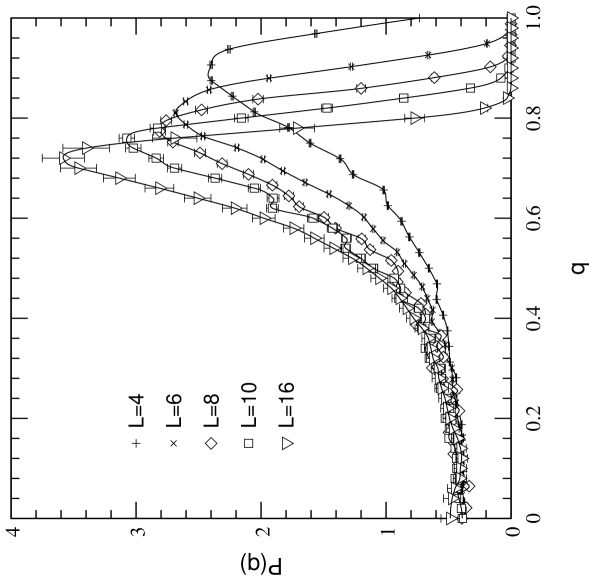
Figure 2: Probability distribution of the overlap $P(q)$ for the $3D$ Ising spin glass with Gaussian couplings. Right to left $L=4,6,8,10$ and $16$ and $T=0.7$.

In figure (2) (from ref. [8]) I show $P(q)$ for the $3D$ Ising spin glass with Gaussian couplings for different lattice sizes. Here $T=0.7$, in the cold phase. Since we are interested in the infinite volume limit we have to look at what happens for increasing lattice size. There are two issues that need to be discussed. The first point is about the region of $P(q)$ for small $q$: a non-zero probability means here that there are stable states with zero overlap. We notice that when increasing the lattice size the non-zero value of the plateau does not change (it would decrease if the transition would become of the ferromagnetic type, and it is shown in [8] that it does increase in a Kosterlitz-Thouless like transition). So, the constant value of the low $q$ plateau is an indication of a non-trivial phase in the infinite volume limit.

The second point is about the location of the peak, that should converge, in the infinite volume limit, to the value Edwards-Anderson value $q_{EA}$ [13]. The location of the peak shifts strongly when increasing the lattice size (we know from a number of numerical experiments that finite size effects are very strong in spin glasses). It is essential to show that the location of the peak does not shift down to $q=0$ when $L\to\infty$.

This can be shown with high confidence level in $4D$ [10] (and again quite clearly but with a larger uncertainty also in $3D$ [8, 9]). In figure (3) we show the location of the peak (for the $4D$ spin glass with binary couplings) at low $T$ (in the broken phase) as a function of $L^{-1.3}$ (the power is hinted by our best fit, see later).

Figure 3: $q_{max}$ versus $L^{-1.3}$ for the $4D$ Ising spin glass with binary couplings.

Already from figure (3) one would consider not plausible a null limiting value, but one has to be careful, and trying to keep the best fit under strict quantitative control. To be more clear one has to exclude, for example, that a fit of the form $A/L^{\alpha}$ could work. This is usually quite tricky, since in a finite $x$ range a small negative power mimics quite well a constant value with corrections given by a higher negative power. In $4D$ even this evidence starts to be quite good [10]: one finds that $q_{max}=0.55+0.86L^{-1.31}$. This is a remarkable piece of quantitative agreement with the mean field theory: the analytic computation of ref. [16] gives for the mean field an exponent of $1.25$ (that is very similar to the $1.31$ we find in $4D$).

To end this section it is also interesting to note that more and more, when increasing $L$, the individual $P_{J}(q)$ (for a given realization of the couplings) show a complex structure and many minima. For example [10] the density of $J$ configurations whose $P_{J}(q)$ has $4$ maxima goes from $0.1$ at $L=3$ up to $.35$ for $L=8$.

3 The Mean Field Picture

3.1 Non Self-Averageness

In the mean field picture one expects that sample to sample fluctuations of some observable quantities do not go to zero in the thermodynamic limit. We have shown numerically in [3] that for example sample to sample fluctuations of $\langle q^{2}\rangle_{J}$ behave in the $3D$ spin glass as one would expect for the mean field. In this same paper we have also noticed (and the same holds for the $4D$ model) that the relation that had been obtained in Mean Field [13]

$$\overline{\langle q^{2}\rangle_{J}\langle q^{2}\rangle_{J}}=\frac{2}{3}\overline{\langle q^{2}\rangle_{J}}\,\,\,\,\overline{\langle q^{2}\rangle_{J}}+\frac{1}{3}\overline{\langle q^{4}\rangle_{J}}\ ,$$ (2)

holds with very good precision for the finite dimensional model. Guerra in ref. [12] has shown that indeed this class of relations has to hold, also for finite dimensional models, under very general hypothesis.

3.2 Correlation Functions and Block Overlap

To establish the pattern of the symmetry breaking one wants to learn about the spatial structure of typical equilibrium configurations. We want to learn about the structure of typical spin domains.

One way to study this problem is to look at spatial correlation functions. Mean field theory tells us that, as we have seen (and found also in the realistic models), the theory has an equilibrium $q=0$ sector. Here one expects a power behavior, i.e. the restricted $q$-$q$ correlation functions behave as

$$\frac{1}{V}\overline{\sum_{i}\langle q_{i}q_{i+x}\rangle}|_{q=0}\approx|x|^{-\alpha}\ .$$ (3)

We have used a dynamic approach to compute these equilibrium correlation functions [3]. We reach a good control, and we observe a clear power behavior. Recently we have confirmed this result with equilibrium simulations [9].

The second check is based on defining the overlap of two configurations in boxes of linear size $R$, $q_{R}(x)\equiv R^{-D}\sum_{y}\sigma_{x+y}\tau_{x+y}$, where $y$ is a vector in a $R^{D}$ box, and checking how does this observable behave when $R$ increases. In an ordinary scaling picture after reaching the typical size of a cluster (for $R\to\infty$, $R\ll L$) the distribution probability of $q_{R}$, $P_{R}(q_{R})$, should peak in two $\delta$-functions at $\pm q_{EA}$. On the contrary in the mean field approach one expects the $P_{R}$ to stay Gaussian on all scales. In our numerical simulations we always observe a clear mean field like behavior.

3.3 Ultrametricity

Ultrametricity is a crucial feature of the Parisi solution (see for example [17]). States appearing in the Parisi solution of the Mean Field SK theory are organized according to an ultrametric structure: if we define a distance among two configurations $d(\alpha,\beta)$ the usual triangular inequality $d(\alpha,\gamma)\leq d(\alpha,\beta)+d(\beta,\gamma)$ is substituted by the stronger inequality $d(\alpha,\gamma)\leq\max\{d(\alpha,\beta),d(\beta,\gamma)\}$, i.e. all triangles have two equal sides longer or equal to the third one. This is the structure one finds when considering, for example a hierarchical tree. One possible definition for the distance of two spin configurations is

$$d(\alpha,\beta)\equiv\frac{q_{EA}-q_{\alpha\beta}}{2q_{EA}}\ .$$ (4)

To study this issue (in $4D$ with binary coupling) [5] we have used a constrained Monte Carlo procedure. We simulate $3$ copies of the system, with the same couplings, and we constrain $2$ of the $3$ overlap to be fix

$$q(\alpha,\beta)=q(\beta,\gamma)=\overline{q}$$ (5)

(in the actual numerical simulation we let $\overline{q}$ vary over a small range). We measure then $q(\alpha,\gamma)$.

Again, the results of the simulation are not distinguishable from the ones one gets for the SK model, and contains strong hints towards the presence of an ultrametric structure. For example we can give a measure of the amount of equilibrium configurations that are not ultrametric by defining

$$I_{L}\equiv\int_{-1}^{\overline{q}}(q_{L}-\overline{q})^{2}P(q_{L})dq_{L}+\int_{q_{EA}}^{1}(q_{L}-q_{EA})^{2}P(q_{L})dq_{L}\ ,$$ (6)

that we expect to go to zero, for $L\to\infty$, if the states have an ultrametric structure. We find that $I_{L}$ has a very clear power behavior, i.e. $I_{L}\approx(-1\pm 5)10^{-4}+(.76\pm.03)/L^{2.21\pm 0.04}$ (where the errors are only statistical). This is again a remarkable agreement with mean field predictions, since from ref. [16] one would expect a value of 8/3 for the mean field theory.

4 Conclusions

Numerical simulations show that the behavior of finite dimensional spin glasses is very similar to the one of the Parisi solution of mean field theory. Together with a qualitative evidence (including the behavior of $P(q)$ and the correlation function) there is some striking quantitative evidence, involving the value of exponents determining finite size corrections. It is maybe worth noticing that where the numerical evidence is not very strong (because of finite size effects or because of the difficulty of thermalizing the system deep in the cold phase) this is true also for actual simulations of the mean field theory. There is, as usual, space for improvements.

References

- [1] E. Marinari, G. Parisi and J. Ruiz-Lorenzo, Numerical Simulations of Spin Glass Systems, in Spin Glasses and Random Fields, edited by P. Young, to be published, cond-mat/9701016.
- [2] E. Marinari, G. Parisi and F. Ritort, J. Phys. A: Math. Gen. 27 (1994) 2687.
- [3] E. Marinari, G. Parisi, F. Ritort and J. Ruiz-Lorenzo, Phys. Rev. Lett. 76 (1996) 843.
- [4] N. Kawashima and A. P. Young, Phys Rev. B 53 (1996) 484.
- [5] A. Cacciuto, E. Marinari and G. Parisi, cond-mat/9608161, to be published in J. Phys. A: Math. Gen..
- [6] M. Picco and F. Ritort, cond-mat/9702041.
- [7] E. Marinari, G. Parisi and F. Zuliani, cond-mat/9703253.
- [8] D. Iniguez, E. Marinari, G. Parisi and J. Ruiz-Lorenzo, cond-mat/9707050, to be published in J. Phys. A: Math. Gen..
- [9] E. Marinari, G. Parisi and J. Ruiz-Lorenzo, The Ising Spin Glass On and Off-Equilibrium, to be published.
- [10] E. Marinari and F. Zuliani, Ising Spin Glass, to be published.
- [11] E. Marinari, Optimized Monte Carlo Methods, lectures given at the 1996 Budapest Summer School on Monte Carlo Methods, to be published by Springer-Verlag, J. Kertesz and I. Kondor editors, cond-mat/9612010.
- [12] C. M. Newman and D. L. Stein, Phys. Rev. Lett. 76 (1996) 515; G. Parisi, cond-mat/9603001; C. M. Newman and D. L. Stein, adap-org/9603001; cond-mat/9612097; F. Guerra, Int. J. Mod. Phys. B 10 (1996) 1675; C. M. Newman in these proceedings.
- [13] M. Mézard, G. Parisi and M. A. Virasoro, Spin Glass Theory and Beyond, (World Scientific, Singapore 1987).
- [14] G. Parisi, Phys. Rev. Lett. 43 (1979) 1754; J. Phys. A: Math. Gen. 13 (1980) 1101; 1887; L115; Phys. Rev. Lett. 50 (1983) 1946.
- [15] E. Marinari, G. Parisi and F. Ritort, J. Phys. A: Math. Gen. 27 (1994) 7631; 27 (1994) 7647; 28 (1995) 327; 28 (1995) 4481.
- [16] S. Franz, G. Parisi and M. Virasoro, J. Phys. I (France) 2 (1992) 1869.
- [17] R. Rammal, G. Toulouse and M. Virasoro, Rev. Mod. Phys. 58 (1986) 765.