Properties of the random field Ising model in a transverse magnetic field

Abstract

We consider the effect of a random longitudinal field on the Ising model in a transverse magnetic field. For spatial dimension $d>2$, there is at low strength of randomness and transverse field, a phase with true long range order which is destroyed at higher values of the randomness or transverse field. The properties of the quantum phase transition at zero temperature are controlled by a fixed point with no quantum fluctuations. This fixed point also controls the classical finite temperature phase transition in this model. Many critical properties of the quantum transition are therefore identical to those of the classical transition. In particular, we argue that the dynamical scaling is activated, i.e, the logarithm of the diverging time scale rises as a power of the diverging length scale.

A number of recent theoretical [1, 2, 3, 4, 5, 6] and experimental [7] works have studied the effects of randomness on simple quantum statistical models. These studies have been motivated by the need to understand in a simple context the interplay of effects related to strong randomness, interactions, and quantum fluctuations. In this paper, we study the effect of a random longitudinal field applied to the transverse field Ising model. The effects of random longitudinal fields on classical Ising models have been studied extensively[8], and are partially well understood. In contrast, very little is known about the corresponding quantum problem in realistic dimensions. Most previous studies of this system have been limited to mean field theory (expected to be valid above $6$ spatial dimensions; see below) or to an expansion in $\epsilon=6-d$. However, as is well known from the classical problem, these results are not expected to directly be of much relevance to physical systems in finite dimensions much smaller than $6$. Here we will provide a general scaling theory applicable in any dimension.

The model in consideration is defined by the Hamiltonian

$${\cal H}=-J\sum_{i,j}\sigma_{i}^{z}\sigma_{j}^{z}-h\sum_{i}\sigma_{i}^{x}-\sum_{i}H_{i}\sigma_{i}^{z}$$ (1)

For simplicity, we have assumed that $J$ and $h$ are non-random, though our results should apply also for weakly random $J$ and $h$. $H_{i}$ is assumed to be random with zero mean and variance $\Delta^{2}$. The $\vec{\sigma}_{i}$ are Pauli spin matrices. We note that, as usual, this quantum model in $d$ dimensions at $T=0$ is equivalent to a classical Ising model in $d+1$ dimensions in a random field with the randomness correlated along one direction.

It will often be more convenient to consider a coarse-grained continuum field theoretic version of the Hamiltonian Eqn. 1. The continuum action is readily written down as:

$$S=\int d\tau\int d^{d}x\frac{1}{t}\left[(\frac{\partial\phi}{\partial\tau})^{2}+(\nabla\phi)^{2}+r\phi^{2}+u\phi^{4}-H(x)\phi(x,\tau)\right]$$ (2)

where $H(x)$ is the (coarse-grained) random field and is taken to be Gaussian distributed with mean $0$ and variance $\Delta^{2}$. For future convenience, we have introduced a factor $t$ as an overall scale for the action.

Later in this paper, we use the standard Imry-Ma argument to show that the ordered phase is unstable to any weak random field for spatial dimension $d\leq 2$. In Fig 1, we show the expected phase diagram for $d>2$ in the temperature ($T$), $h$, $\Delta$ space. In what follows, we will concentrate primarily on the $T=0$ transition from the ordered phase to the paramagnetic phase. Our central claim is that the quantum transition is controlled by a fixed point with no quantum fluctuations in any dimension ($>2$). However quantum fluctuations are “dangerously irrelevant” at this fixed point, and need to be included to get the correct critical behaviour of many physical observables. Such fluctuationless fixed points have arisen in several other recent studies of quantum transitions in random systems[1, 9, 5, 6, 10]. For the model in consideration here, this claim is completely analogous to the corresponding claim on the role of thermal fluctuations at the finite temperature phase transition in classical random field Ising magnets[8]. Indeed, we claim that the same fixed point controls both the classical (finite $T$) and quantum ($T=0$) transitions in this model. This enables us to relate many of the critical properties of the quantum transition to those of the well-studied (but only partially understood) classical transition. In particular, we suggest that the dynamical scaling is activated, i.e, the logarithm of the diverging time scale rises as a power of the diverging length scale.

I Weak randomness

We first consider the effects of weak random fields on the properties of the pure system. These are quite innocuous deep in the paramagnetic phase when the transverse field wins over both the randomness and the exchange interaction. So we will turn immediately to the ordered phase and the critical point.

It is easy to see using the Imry-Ma[11, 12, 13] argument that for dimension $d>2$, the ordered phase of the quantum model is stable to a weakly random $H_{i}$. Imagine that in the absence of randomness, the system is deep in the ordered phase. The stability to a weak random field is determined by balancing the energy cost to form large-sized domains with the typical energy gain because of the random $H_{i}$. Deep in the ordered phase, the energy cost of a domain $\sim L^{d-1}$ while the typical energy gain due to the random field $\sim L^{d/2}$ exactly as in the classical problem. Thus for $d>2$, for weak enough random fields, it is not favourable to form large-sized domains and the system stays ordered. We expect of course that strong randomness will destroy the ordered phase in any dimension. Precisely in $d=2$, as in the classical problem, the system is marginally unstable and there is no ordered phase.

Now, assume that we are at the critical point of the pure system in $d>2$. When are weak random fields a relevant perturbation at this critical fixed point? This can be answered as follows. Consider the continuum action Eqn. 2. Averaging over the disorder using replicas gives the term $\frac{\Delta^{2}}{2}\int d^{d}x\int d\tau_{1}d\tau_{2}\sum_{a,b}\phi_{a}(x,\tau_{1})\phi_{b}(x,\tau_{2})$. Now under the renormaliation group transformation appropriate to the critical fixed point of the pure system $x\rightarrow x^{\prime}=\frac{x}{s}$, $\tau\rightarrow\tau^{\prime}=\frac{\tau}{s^{z}}$, and $\phi\rightarrow\phi^{\prime}=\phi s^{\frac{d+z-2+\eta}{2}}$. This gives $\Delta^{2\prime}=\Delta^{2}s^{z+2-\eta}$. Clearly then $\Delta$ is always relevant.

II The critical fixed point

In this section, we will present the reasoning behind our assumption that the fixed point controlling the transition has no quantum fluctuations[14].

For classical random field magnets, it is believed[8] that the properties of the finite temperature phase transition (which exists for $d>2$) are controlled by a zero temperature fixed point. The first evidence for this belief came from perturbative studies[11, 15] of a continuum field theoretic description of the magnet near the critical point. Order by order in perturbation theory, it can be shown that the effects of the fluctuations introduced by the randomness dominate over the effects of the thermal fluctuations near the critical point. This is interpreted in renormalization group language to be a manifestation of a zero-temperature fixed point with (dangerously) irrelevant thermal fluctuations. Though many of the predictions of this perturbative analysis are believed not to be correct for realistic dimensions ($d=2$,$3$), there is a general consensus that the critical fixed point is fluctuationless in all dimensions where there is a transition. This is further supported by heuristic renormalization group arguments valid in $d=2+\epsilon$[16], numerical real space renormalization calculations[17], and general agreement of some of the phenomenology suggested by such fluctuation-less fixed points with experiments in $d=3$[18].

For the quantum random field magnets that we are considering here, a similar perturbative analysis, valid in high dimension, of a continuum field theory expected to describe the correct $T=0$ critical behaviour was undertaken several years ago by two groups[19, 20](See also Section IV). Again it was found that order by order in perturbation theory, the effects of fluctuations introduced by the randomness dominated the effects of quantum fluctuations. We take this to be strong evidence that the fixed point is fluctuationless for every dimension ($d>2$) for the quantum problem as well.

Now consider the finite temperature phase transition in the quantum model which occurs when the ground state is ordered. This transition is, of course, in the same universality class as that in the classical models discussed earlier. It is clear that this is controlled by the same fixed point that controls the quantum transition. Thus, we have the unusual situation that the same fixed point controls both the $T=0$ and $T\neq 0$ transitions. The phase diagram and RG flows (for $d>2$) are shown in Figure 1.

III General Scaling Hypothesis for $2<d<6$

A number of results follow from the claim that the same fixed point controls both the classical and quantum transitions. First, on approaching the transition from the ordered phase, the magnetization vanishes with an exponent $\beta_{Q}$ which is the same as for the classical transition. Next consider correlation functions. As in the classical problem, there are two different correlation functions that can be defined: The correlation function

$$C(x,\tau;x^{\prime},\tau^{\prime})=\overline{<\sigma_{z}(x,\tau)><\sigma_{z}(x^{\prime},\tau^{\prime})>}-\overline{<\sigma_{z}(x,\tau)>}~{}\overline{<\sigma_{z}(x^{\prime},\tau^{\prime})>}$$ (3)

where the angular brackets denote averaging over quantum fluctuations and the overline denotes averaging over the randomness. As the randomness is independant of time, the system is translationally invariant in time in every sample. Therefore $C(x,\tau;x^{\prime},\tau^{\prime})$ is independant of $\tau,\tau^{\prime}$ and we will refer to it as $C(x,x^{\prime})$ from now on. After averaging over the disorder, spatial translational invariance is also restored in the correlation function, and so $C(x,x^{\prime})=C(x-x^{\prime})$. This satisfies (near the transition)

$$C(x)\sim\frac{1}{x^{d-2+\overline{\eta}_{Q}}}{\cal C}\left(\frac{x}{\xi}\right)$$ (4)

where the correlation length $\xi\sim|h-h_{c}|^{-\nu_{Q}}$. The scaling function ${\cal C}$ and the exponents $\nu_{Q}$, $\overline{\eta}_{Q}$ are properties of the fixed point theory and its relevant perturbations (the deviation from the critical randomness strength). As these are the same for both the quantum and classical transitions, we get the result that the exponents $\nu_{Q}$, $\overline{\eta}_{Q}$, and the function ${\cal C}$ are identical to their classical counterparts.

The connected correlation function

$$G_{c}(x,\tau;x^{\prime},\tau^{\prime})=\overline{<T_{\tau}(\sigma_{z}(x,\tau)\sigma_{z}(x^{\prime},\tau^{\prime}))>-<\sigma_{z}(x,\tau)><\sigma_{z}(x^{\prime},\tau^{\prime})>}$$ (5)

where $T_{\tau}$ is the time-ordering symbol. Clearly $G_{c}(x,\tau;x^{\prime},\tau^{\prime})=G_{c}(x-x^{\prime},\tau-\tau^{\prime})$.

Note that this correlation function vanishes at the fixed point (as there are no quantum fluctuations at the fixed point). Thus to obtain its critical behaviour, we need to keep the irrelevant quantum fluctuations. Similarly for the corresponding classical problem, it is necessary to keep the irrelevant thermal fluctuations. As these two irrelevant perturbations may have quite different effects, in general, we do not expect $G_{c}$ to scale identically to the classical space and time dependant correlation function.

However it is possible to argue that the static correlation function of the quantum problem scales identically to the equal-time correlation function of the classical problem. This was first noticed within the $\epsilon$ expansion by Boyanovsky and Cardy[20], but as we show below is more generally valid (though other results of the $\epsilon$ expansion are not). Consider the susceptibility[21]of the model to an external spatially varying static magnetic field $H_{ext}(x)$. Clearly for both the quantum and classical problems, the scaling of this susceptibility near the transition is just determined by minimizing the classical fixed-point Hamiltonian in the presence of the external field. Hence the static (non-local) susceptibilility scales identically for the classical and quantum problems. Now at any finite $T\neq 0$ in the classical problem, the fluctuation-dissipation theorem implies that the equal-time correlation function is proportional to the susceptibility. Similarly, the static correlation function of the quantum problem is also proportional to its susceptibility. Thus these two correlation functions scale identically. We then have the result

$$\int d\tau G_{c}(x,\tau)\sim\frac{1}{x^{d-2+\eta}}\tilde{{\cal G}}\left(\frac{x}{\xi}\right)$$ (6)

with $\eta$ and the scaling function $\tilde{{\cal G}}$ being identical to those for the connected equal-time correlation functions of the classical problem. The equal-time correlation function in the quantum problem will however scale differently.

We now turn to dynamical correlations. For the classical transition, Villain and Fisher[22] have presented arguments to show that the dynamical scaling is unconventional, with the logarithm of the characteristic relaxation times scaling as a power of the length scales. Similar unconventional dynamic scaling also occurs in the vicinity of the random quantum transitions studied recently[1, 5, 6], all of which are controlled by fluctuation-less fixed points. We suggest below that the dynamic scaling is activated at this quantum transition as well.

The argument for the dynamic scaling closely follows that for the classical case. Consider a block of the system of size $\sim\xi$ near the critical system. Ignoring quantum fluctuations, the energy landscape as a function of the total magnetization of the block has been argued to scale as $\xi^{\theta}$[22]. Most blocks would thus have a single deep global minimum at some non-zero value of the magnetization. The energy of this minimum will differ from those of other local mimima by amounts $\sim\xi^{\theta}$. The barriers separating these different local mimima also scale as $\xi^{\theta}$. Effects of quantum fluctuations on such blocks should be rather small, and do not contribute significantly to the dynamics. However, there would be some rare blocks in which there are two minima with an energy separation which is nearly zero. The dynamics at long time scales will be dominated by quantum tunnelling between such minima in these rare blocks. As the barrier between these minima rises as a power of $\xi$, it is natural that the tunneling time $t_{Q}\sim\exp(c\xi^{\psi})$ with $\psi$ a new exponent. (This quantum tunneling will be important so long as the energy difference between the two minima is roughly less than $\hbar/t_{Q}$). Thus the dynamics is activated like in the other random quantum transitions studied in Refs [1, 5, 6].

This therefore motivates the following scaling form for the imaginary part of the $q,\omega$ dependant susceptibility (which is the spectral density for the connected correlator introduced above):

$$\chi^{\prime\prime}(q,\omega)=\xi^{\kappa}f(q\xi,\frac{\ln{\frac{1}{\omega t_{0}}}}{\xi^{\psi}})$$ (7)

where $t_{0}$ is a microscopic time scale. The exponent $\kappa$ will be related to other exponents below. The real part of the susceptibility may be obtained by the Kramers-Kronig relation:

$$\chi^{\prime}(q,\omega)=\int\frac{d\omega^{\prime}}{\pi}\frac{\chi^{\prime\prime}(q,\omega^{\prime})}{\omega^{\prime}-\omega}$$

Following Pytte and Imry[23], we write $y=\frac{\ln{\frac{1}{\omega^{\prime}t_{0}}}}{\xi^{\psi}}$ and $z=\frac{\ln{\frac{1}{\omega t_{0}}}}{\xi^{\psi}}$. Then

$$\chi^{\prime}(q,\omega)=\xi^{\kappa+\psi}\int_{-\infty}^{+\infty}\frac{dy}{\pi}f(q\xi,y)\left[\frac{1}{e^{\xi^{\psi}(y-z)}+1}-\frac{1}{e^{\xi^{\psi}(y-z)}-1}\right]$$

In the scaling limit when $\xi\rightarrow\infty$, we may approximate

$$\frac{1}{e^{\xi^{\psi}(y-z)}+1} \approx \theta(z-y)$$

$$\frac{1}{e^{\xi^{\psi}(y-z)}-1} \approx -\theta(z-y)$$

Thus

$$\chi^{\prime}(q,z)\sim\frac{2}{\pi}\xi^{\kappa+\psi}\int_{-\infty}^{z}dyf(q\xi,y)$$

Thus we get the following scaling form for the real part:

$$\chi^{\prime}(q,\omega)\sim\xi^{\kappa+\psi}\tilde{f}(q\xi,\frac{\ln{\frac{1}{\omega t_{0}}}}{\xi^{\psi}})$$ (8)

with $\tilde{f}(x,z)=\frac{2}{\pi}\int_{-\infty}^{z}dyf(x,y)$. In particular, the static susceptibility

$$\chi^{\prime}(q,0)\sim\xi^{\kappa+\psi}\tilde{f}(q\xi,-\infty)$$

Thus we identify $\kappa=2-\eta-\psi$. Note that similar scaling forms apply for the dynamics near the classical transition as well, although with a different value for $\psi$ and a different scaling function $f(x,y)$. Nevertheless, as we argued earlier the function $\tilde{f}(x,-\infty)$ should be the same for the quantum and classical transitions.

IV Expansion in $\epsilon=6-d$

As shown below, the upper critical dimension of this model is $6$. It is natural to try an expansion in powers of $\epsilon=6-d$. This was done long back by Aharony, Gefen and Shapir[19] and by Boyanovsky and Cardy[20]. Here, we will review their results and discuss them in the context of the general scaling hypotheses of the previous section.

The $\epsilon$ expansion is done using the continuum action Eqn. 2. It is instructive to set up the renormalization group so that $t$ is allowed to flow while keeping the strength of the randomness fixed. In particular, the results of Ref. [19, 20] show that $t$ flows to zero at the critical fixed point. When $t=0$, the partition function is determined by the particular configuration $\phi(x,\tau)$ that minimizes the action. Clearly the minimum action configuration is static. Thus solving the fixed point theory simply corresponds to finding the static configuraion $\phi_{stat}(x)$ that minimizes the potential energy terms in the action. Thus the fixed point theory is entirely classical.

First consider the Gaussian theory with $u=0$. The correlation functions $C(k,\omega)=\overline{\langle\phi(k,\omega)\rangle\langle\phi(-k,-\omega)\rangle}$ and $G(k,\omega)=\overline{\langle\phi(k,\omega)\phi(-k,-\omega)\rangle-\langle\phi(k,\omega)\rangle\langle\phi(-k,-\omega)\rangle}$ can be easily calculated. The result is:

$$C(k,\omega) = \frac{\Delta^{2}\delta(\omega)}{k^{2}+r}$$

$$G(k,\omega) = \frac{t}{k^{2}+\omega^{2}+r}$$

The critical point is at $r=0$. The correlation functions introduced in the previous section are seen to scale as

$$C(x) \sim \frac{1}{x^{d-4}}{\cal C}(\frac{x}{\xi})$$ (9)

$$G_{c}(x,\tau) \sim \frac{1}{x^{d-1}}{\cal G}(\frac{x}{\xi})$$ (10)

with the correlation length $\xi=\frac{1}{\sqrt{r}}$. Thus, in the Gaussian theory, we have $\nu_{Q}=\frac{1}{2}$, $\eta_{Q}=0$, $\overline{\eta_{Q}}=-2$. Note that for the classical problem also, the Gaussian exponents are $\nu=\frac{1}{2}$, $\eta=0$, $\overline{\eta}=-2$. This is a trivial illustration of the general point made in the previous section. The dynamic scaling is however conventional in the Gaussian theory.

Now consider a momentum shell renormalization group transformation on the Gaussian action. It is convenient to let $t$ flow and keep the strength $\Delta$ of the random field fixed. The flow equations for $t$ and $r$ are readily seen to be

$$\frac{dt}{dl} = -3t$$

$$\frac{dr}{dl} = 2r$$

Thus even in the Gaussian theory, $t$ flows to $0$ at the fixed point which is hence fluctuationless. The tree-level flow equation for $u$ at the Gaussian fixed point is just obtained by power-counting and is

$$\frac{du}{dl}=(6-d)u$$

Thus interaction effects are irrelevant above $6$ spatial dimensions and the Gaussian theory gives the true critical behaviour. For $d$ below $6$, it is possible to construct an expansion in powers of $\epsilon=6-d$[19]. To leading order, the one loop RG equations are:

$$\frac{dt}{dl} = -3t$$

$$\frac{dr}{dl} = 2r+\frac{3ut}{2}K_{d}\Lambda^{d-1}(1-\frac{r}{2\Lambda^{2}})+6u\Delta K_{d}\Lambda^{d-6}(1-\frac{3r}{\Lambda^{2}})$$

$$\frac{du}{dl} = (6-d)u-\frac{9u^{2}t}{4}K_{d}\Lambda^{d-3}-36u^{2}\Delta K_{d}\Lambda^{d-6}$$

where $\Lambda$ is the high-momentum cutoff and $K_{d}=\frac{S_{d}}{(2\pi)^{d}}$. ($S_{d}$ is the surface area of a unit sphere in $d$ dimensions). Again $t$ flows to $0$ at the fixed point. Setting $t=0$ in the remaining equations it is clear that there is a non-trivial fixed point at $r*=-\frac{\epsilon\Lambda^{2}}{12},u*=\frac{\epsilon}{36\Delta K_{6}}$. The flows can be linearized around this fixed point and give, for instance, $\nu=\frac{1}{2}+\frac{\epsilon}{12}$ to first order in $\epsilon$. Note that this is the same as for the pure problem in $3-\epsilon$ dimensions. This is a general feature of the $\epsilon$ expansion - all the exponents characterizing static critical properties in $d$ dimensions are the same as the pure problem in $d-3$ dimensions. This result however is an artifact of the $\epsilon$ expansion and is not true in all dimensions.

The fact that $t$ flows to $0$ to this order means that the new non-Gaussian fixed point is also fluctuationless. In fact the flow equation for $t$ has been shown to be exact to all orders in $\epsilon$[19, 20]. Thus at least within the $\epsilon$ expansion, the fixed point is fluctuationless in any dimension.

It was argued by Boyanovsky and Cardy that all the exponents and scaling functions associated with static critical properties of the quantum transition were the same as for the classical transition. As we have seen in the previous section, this result is true quite generally. However dynamic properties (for instance time-dependant correlation functions) were shown to scale differently. Within the $\epsilon$ expansion, they found that the dynamic scaling is conventional at both transitions with $z_{Q}=1+(0.0185)\epsilon^{2}+(0.0182)\epsilon^{3}+o(\epsilon^{4})$ and $z_{cl}=2z_{Q}$. Thus, as in the classical case, the $\epsilon$ expansion is qualitatively incorrect to describe many aspects of the critical behaviour of the random field quantum system well below the upper critical dimension. Nevertheless the $\epsilon$ expansion provides useful evidence for the claim that the fixed point has no quantum fluctuations.

V Discussion

What we have done in this paper is primarily to update the theory of the quantum random field models since the pioneering papers in Ref.[19, 20], to take into account subsequent develoments in the understanding of the classical problem. Our main assumption, motivated by the results of Ref.[19, 20], was that the quantum transition in any dimension is controlled by a fluctuationless fixed point that also controls the classical finite temperature transition. Some of the consequences of this assumption were then examined. The static critical properties of the quantum transition are identical to those of the classical transition. The dynamics (which depends on the irrelevant quantum/thermal fluctuations) is similar, though not identical. In particular, we suggested that the dynamic scaling is of the activated form, with the length scales depending logarithmically on time scales. We have however not provided calculational evidence for this suggestion. Evidence for the activated dynamic scaling cannot be obtained from the $\epsilon$ expansion (or from other perturbative approaches like a $2+\epsilon$ expansion). Even for the classical transition, the only available evidence comes from numerical calculations[24] and agreement with the phenomenology seen in experiments[18]. Here, we have argued that activated dynamics in the quantum case is natural if it occurs in the classical problem. We may therefore regard support for activated dynamics in the classical transition as some sort of support for it happening in the quantum transition as well.

There are some other important questions that are left open. For most of the paper, we have focused on the critical point. The paramagnetic phase should be interesting to study by itself. In particular, is there a finite gap all the way till the critical point, or is there a Griffiths-phase with gapless excitations in the vicinity of the critical point? It is possible to show[25] for the quantum version of a special model introduced by Grinstein and Mukamel[26] in $d=1$ that the spin-autocorelation in imaginary time has a stretched exponential form $e^{-c\tau^{\frac{1}{3}}}$. This implies gapless excitations with an essential singularity at zero energy in the local density of states. For more realistic models however, even in $d=1$, the autocorrelation presumably decays exponentially. The general situation is unclear. Similar questions can also be asked about Griffiths effects for the uniform susceptibility in the paramagnetic phase.

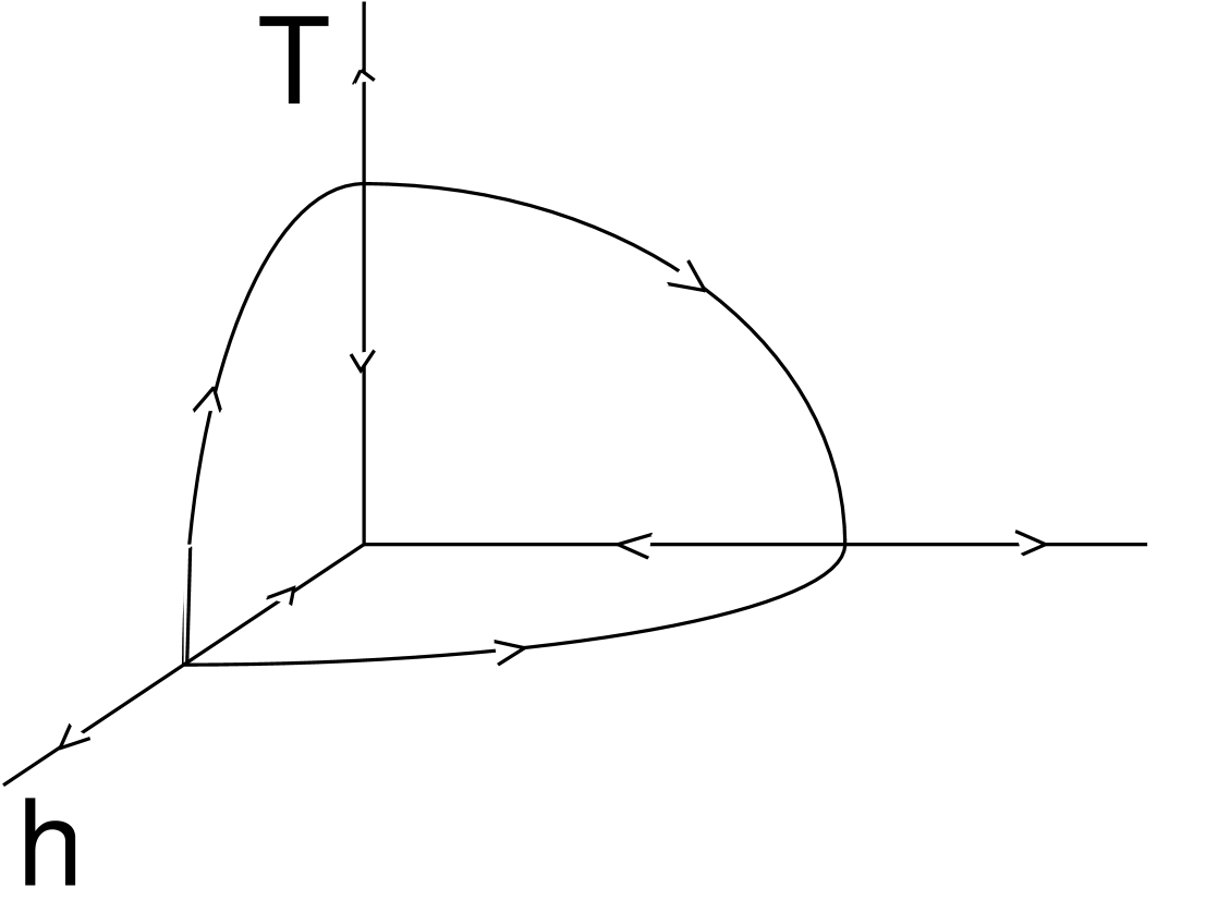
FIG. 1.: Schematic phase diagram and renormalization group flows for the transverse field Ising model in a random longitudinal field for $d>2$ in the temperature($T$), transverse field($h$), strength of randomness($\Delta$) space. There is a transition from a ferromagnet to a paramagnet as any of these three parameters is increased.

- [1] D.S. Fisher,Phys. Rev. Lett. 69, 534 (1992); D.S. Fisher,Phys. Rev. B51, 6411 (1995); A.P. Young and H. Rieger, cond-mat/9510027
- [2] J.Miller and D.Huse, Phys. Rev. Lett. 70, 3147 (1993); J.Ye, S.Sachdev, and N.Read, Phys. Rev. Lett. 70, 4011 (1993); M.J. Thill and D.A. Huse, Physica A15, 321 (1995); N. Read, S. Sachdev, and J. Ye , Phys. Rev. B 52, 384 (1995) ;
- [3] S. Sachdev and J. Ye, Phys. Rev. Lett. 69, 2411 (1992)
- [4] M. Guo, R.N. Bhatt, and D.A. Huse, cond-mat/9605111; H. Rieger and A.P. Young, cond-mat/9512162
- [5] T. Senthil and S.N. Majumdar, Phys. Rev. Lett. 76, 3001 (1996)
- [6] T. Senthil and S. Sachdev, Phys. Rev. Lett., 77, 5292 (1996).
- [7] W. Wu, B. Ellman, T.F. Rosenbaum, G. Aeppli, and D.H. Reich, Phys. Rev. Lett. 67, 2076 (1991); W. Wu, D.Bitko, T.F. Rosenbaum, and G. Aeppli, Phys. Rev. Lett. 71, 1919 (1993)
- [8] See T.Nattermann, cond-mat/9705295 for a recent review of the theory of classical random field magnets.
- [9] S. Sachdev, N. Read, and R. Oppermann, Phys. Rev. B 52, 10286 (1995).
- [10] T.R. Kirkpatrick and D. Belitz, Phys. Rev. Lett. 74, 1178 (1995).
- [11] Y. Imry and S.-k. Ma, Phys. Rev. Lett. 35, 1399 (1975)
- [12] For classical random field Ising systems, the question of the lower critical dimension was the subject of a long-standing controversy as field theoretic arguments seemed to predict that any weak random field destroys LRO for all dimensions less than three in disagreement with the Imry-Ma argument. This was finally resolved, in favor of the Imry-Ma prediction, by a rigorous proof by Imbrie[13] that the classical random field Ising model is ordered for sufficiently weak randomness.
- [13] J.Z. Imbrie, Phys. Rev. Lett. 53, 1747 (1984); Commun. Math. Phys. 98, 145 (1985).
- [14] We are always also assuming that the transition remains second order in the presence of the random field.
- [15] A. Aharony, Y. Imry and S.-k. Ma, Phys. Rev. Lett., 37, 1364 (1976); G. Grinstein, Phys. Rev. Lett., 37, 944 (1976).
- [16] A.J. Bray and M.A. Moore, J. Phys. C18, L927 (1985)
- [17] See for instance Newman et. al., Phys. rev. B48, 16533 (1993).
- [18] See D.P. Belanger, cond-mat/9706042 for a recent review of experiments on classical random field magnets.
- [19] A. Aharony, Y. Gefen, and Y. Shapir, J. Phys. C15, 673 (1982)
- [20] D. Boyanovsky and J.L. Cardy, Phys. Rev. B27, 5557 (1983).
- [21] It is in principle possible that the susceptibility to a uniform external field is divergent in the vicinity of the transition (as happens in a Griffiths phase) thereby invalidating linear response theory. However we expect that for a generic non-uniform field, the susceptibility will be finite and linear response valid.
- [22] J. Villain, J. de Phys., 46, 1843 (1985); D.S. Fisher, Phys. Rev. Lett., 56, 416 (1986)
- [23] E. Pytte and Y. Imry, Phys. Rev. B 35, 1465 (1987)
- [24] A.T. Ogielski and D.A. Huse, Phys. Rev. Lett. 56, 1298 (1986)
- [25] T. Senthil, unpublished
- [26] Grinstein and Mukamel, Phys. Rev. B27, 4503 (1983)